Dynamic Relaxation Method for Load Capacity Analysis of Reinforced Concrete Elements

Faculty of Civil Engineering and Geodesy, Military University of Technology, 2 Gen. W. Urbanowicza Street, 00-908 Warsaw, Poland
*
Author to whom correspondence should be addressed.
Appl. Sci. 2018, 8(3), 396; https://doi.org/10.3390/app8030396
Submission received: 30 January 2018
/
Revised: 26 February 2018
/
Accepted: 6 March 2018
/
Published: 8 March 2018
(This article belongs to the Section Materials Science and Engineering)
Abstract
:Featured Application
predicting the development of structural elements failure and analysis of the construction systems’ safety, the dynamic analysis of structures with damping.
Abstract
In this paper, an analysis method for the nonlinear behavior of reinforced concrete elements subjected to short-term static loads is proposed. The range of inelastic properties for the structural materials is considered, and the deformation processes of reinforced concrete bar elements are modeled. The structural material properties are modeled using the assumptions from plastic flow theory. The load capacity analysis method for the structural system is developed using the finite difference method. The dynamic relaxation method with critical damping allows for describing the static behavior of a structural element, which is used to solve the nonlinear equilibrium equations. To increase the effectiveness of the method for post-critical analysis, the arc-length parameter on the equilibrium path is included. Numerical experiments for a reinforced concrete beam and eccentrically loaded column are run. Comparative analysis with previously published experimental, numerical, and analytical results demonstrated that the proposed computational method is very effective.
1. Introduction
The effort analysis of structural elements made of concrete using different types of reinforcement is the subject of various studies. These studies differ in scope, scale, and detail degree of analysis. Detailed experimental, analytical or numerical analyses were generally made for single structural elements. For example, the latest investigations on beams were presented in [1,2]. The analysis of steel and concrete composite shear walls under static compression was presented in [3] and under seismic action in [4]. The experimental and numerical analysis of the concrete circular plates with steel fibers reinforcement under impact load was presented in [5]. The latest analytical and experimental load capacities investigations regarding the new concept of composite steel-reinforced concrete floor slab, was presented in [6]. A numerical analysis of reinforcement concrete frame corners under an opening bending moment taking into account the assumed loading time was presented in [7]. In turn, analyses of complex building structures were conducted at a generalized level, which showed a global effort of the construction. The numerical analyses of multistory buildings behavior under exceptional loads were presented in [8,9].
In many studies, the nonlinear analysis of the reinforced concrete structural elements were provided on the basis finite element method using existing software. The non-linear analysis of the shear failure mechanism of reinforced concrete beams was presented in [10,11]. The nonlinear analysis carried out a using numerical algorithm for the reinforced concrete shells under static and dynamic loading were presented in [12]. The numerical analysis including material and geometrical nonlinearity with the influence of shear strength complementary mechanism for the reinforced concrete beams and frame were presented in [13].
A load capacity analysis technique for a structural system was developed using the finite difference method, and the dynamic relaxation method (DRM) was applied to solve the nonlinear equilibrium equations. In this method, the problem can be reduced to analysis of a pseudo-dynamic process by considering critical damping as an aperiodic motion that approaches the equilibrium state under the acting load. The solution to this problem can be obtained using an iterative process with pseudo-time steps. The DRM is used to analyze highly nonlinear problems [14,15,16]. Rezaiee-Pajand and Alamatian [17] proposed further modifications in order to improve the convergence and accuracy of the solutions. Several practical applications of the DRM for structures were presented by Rezaiee-Pajand and Sarafrazi [18], Bel Hadj Ali et al. [19], and Barnes et al. [20].
The arc-length parameter on the equilibrium path was introduced to the proposed numerical procedure to increase the efficiency of the method. This is referred to as the arc-length method, and it simultaneously determines the displacements and load parameter by tracing the equilibrium path that contains the local singular points. Subsequent developments and interpretations of the arc-length method were presented by de Borst et al. [21], among others. A combination of the dynamic relaxation and arc-length methods was presented by Pasqualino [22]. This was then applied to practical analysis of structural members by Ramesh and Krishnamoorthy [23] as well as Pasqualino and Estefen [24].
The literature review leads to the following conclusions. Previous DRM studies mainly focused on the elastic analysis of the structural elements. Wriggers noted that the DRM can describe non-linear static problems but did not give any examples in Reference [25]. A combination of dynamic relaxation and arc-length methods has also been proposed [23,26], and has been further combined with the finite difference method in Reference [22]. These solutions allow for a post-critical analysis, but previous research considered elastic behaviors of homogeneous bar elements for range of geometrical nonlinearities [23] or elastic–plastic behaviors of shell type structures [24]. These previously published papers did not investigate the inelastic range of deformations in reinforced concrete elements. In particular, the studies did not provide solutions for reinforced concrete columns that include the full range of deformations until failure.
In this paper, a general computational algorithm that is based on developed effort analysis methods for reinforced concrete elements was proposed. The main purpose of this work was to develop a computational model of reinforced concrete bar elements, which can be used to study the behavior of an element going from purely elastic to elastic-plastic and then to stress the softening and failure of the cross-section.
To obtain a solution, the modeling range of the inelastic material properties, the deformation processes of the bar structural elements, and the numerical solutions must be considered. The properties of the structural material were modeled by assuming a reduced plane in a compressive/tensile stress state with shear. An elastic-plastic material model with hardening for the reinforcing steel was used. The elastic-plastic material model was developed by considering the stress softening and degradation of the deformation modulus for the concrete. Analysis of the structural element includes a description of the behavior of an eccentrically compressed reinforced concrete element, which was modeled as a bar system under static loading. The equations for moderately large displacements of the bar include the influence of the longitudinal deformations, changes to the rotation angle of the cross-section (curvature), and isochoric strains. These equations were used as the basis of a theoretical model for the behavior of the structural element.
This technique was implemented into the own computer program to calculate strains, stresses, internal forces, and displacements.
To verify the accuracy of the proposed method, numerical studies of bar structural elements were carried out. The simulations considered a bent reinforced concrete beam that was tested experimentally by Buckhouse [27,28] and an eccentrically compressed reinforced concrete column that was tested experimentally and analytically by Lloyd and Rangan [29].
Obtained numerical results were compared with the results of experimental, analytical, and theoretical works from the existing literature.
2. Modeling of Structural Materials
2.1. Reinforcing Steel
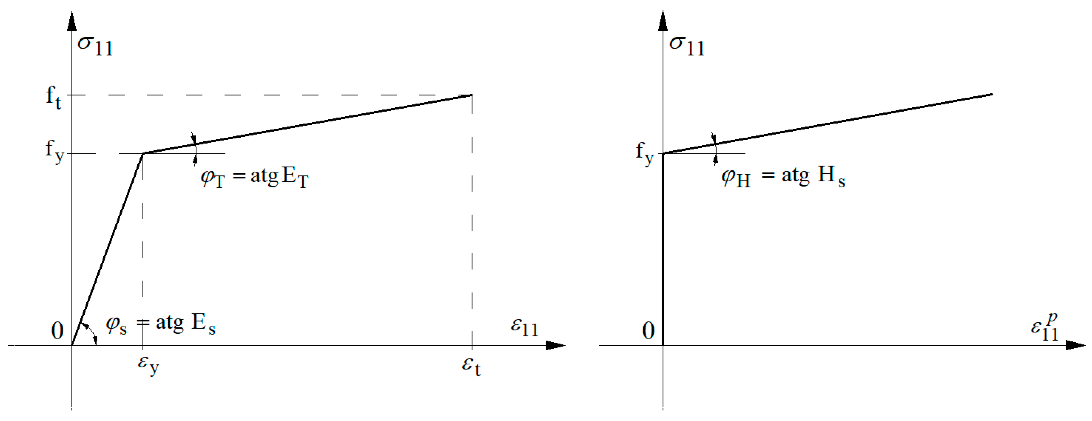
The elastic-plastic model with regard to material hardening was applied for the reinforcing steel, which is shown in Figure 1. The reduced plane stress state (compression/tension with shear) was considered, because of the nature of the reinforcing slender bars in the reinforced concrete element. The stress state in subsequent load steps is described by the equations below.
where is the deformation modulus of steel, is the shear modulus, is the initial Poisson’s ratio , , , and are the known strains and strain increments. is the scalar multiplier that defines the state of stress according to the associated plastic flow rule for the Huber-Mises-Hencky yield criterion, is the step number of the instantaneous strain-stress state in a subsequent time instant, and , and is the time step increment.
To determine the scalar multiplier , the value of the plasticity function must be checked for consistency with the Huber-Mises-Hencky yield criterion:
where is the stress intensity, and is the hardening function of the steel yield limit.
The variation of the steel yield limit function describes the law of isotropic hardening:
where is the effective plastic strain, is the increment of the effective plastic strain, is the steel yield limit for tension/compression, is the steel plastic hardening modulus, and is the time instant when the steel yield limit is achieved.
The uniaxial idealization for the tensile/compressive test is shown in Figure 1. After applying the assumption of elastic and plastic strain increments , where , and , the steel plastic hardening modulus is shown in the equation below.
The tangent deformation modulus of steel is , where is the steel tensile/compressive strength, is the maximum elastic strain, and is the strain that is related to the steel strength.
In the initial assumption , if , or and , we have a purely elastic stress state (or unloading). represents an elastic–plastic state for which the multiplier value is determined from the conditions below.
These equations can be numerically solved using Newton’s method. The solution at the i-th iteration is shown below.
for the assumed accuracy . That is:
The numerical solution of the nonlinear algebraic Equation (6) is well-conditioned. There is only one root such that , which describes the elastic-plastic stress state of Equation (1).
2.2. Concrete
An elastic–plastic material model for concrete that considers material softening and the degradation of the deformation modulus was developed. A reduced plane stress state for the compression/tension range with shear was assumed.
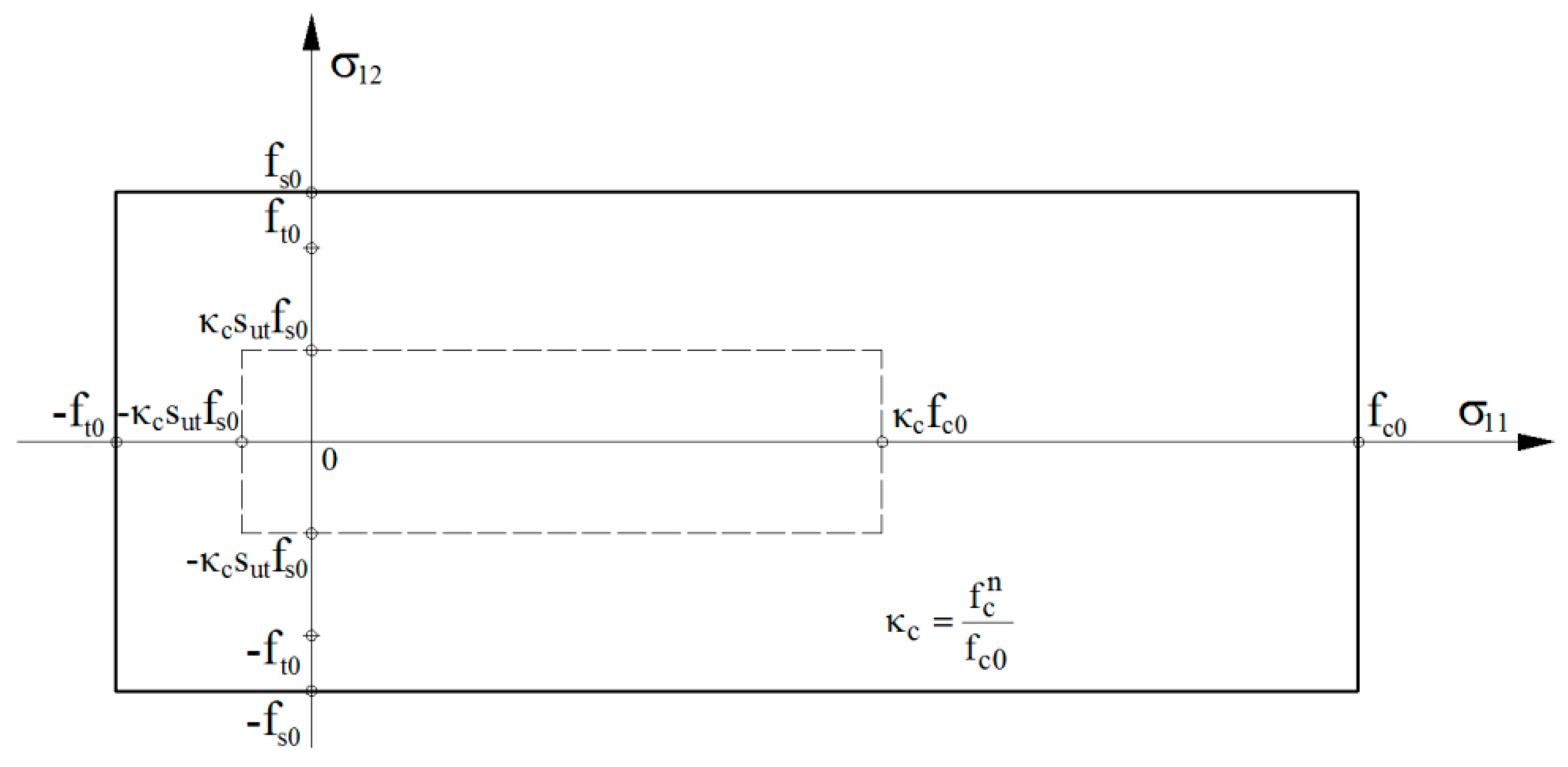
Figure 2 shows an idealization of the concrete model for the plane , where , , and are the initial compressive, tensile, and shear strengths, is the initial modulus of deformation, and are the elastic limit strains in compression and tension, and are the strain limits for the perfectly plastic flow and the material softening range in compression, and is the strain limit for the material softening range in tension.
The concrete model describes the incremental equations for stresses while considering the limitations that result from the yield condition. The stress state in subsequent load steps is described by the relations below.
where is the instantaneous step of the stress-strain state, , , , and are the known strains and strain increments, is the shear deformation modulus, and is the initial Poisson’s ratio. The variable parameters and are described according to schemes presented in Figure 2 and Figure 3, respectively.
The yield criterion that is used in the concrete model is consistent with experimental results for the reduced plane stress state. This is also confirmed by comparing the proposed model with the model described by Stolarski [30], which was calibrated using experimental results.
3. Fundamental Equations
3.1. Equations of Motion
The analysis includes the behavior of bent and eccentrically compressed reinforced concrete elements. The elements are modeled using a system of plane bars and takes into account the initial curvature. The bar system is statically loaded with a short-term longitudinal force, bending moment, uniformly distributed load, and concentrated forces acting on the plane perpendicular to the longitudinal axis of the element.
This reinforced concrete element considers specific geometrical factors including the variable cross-sectional distribution of concrete and reinforcing steel areas, the initial curvature, and the boundary conditions that result from the support and external load.
The equations of dynamic motion for a reinforced concrete bar element that is characterized by the unit mass (), the unit mass of inertia , and the unit damping coefficients for the displacements and rotations were derived. The problem of the damping coefficient estimation was detailed in the paper [33].
The differential equilibrium equations were defined in the global Cartesian coordinate system , as shown in Figure 4, where is the length of the deformed element, and is the slope angle. They have the form shown below.
where is the internal longitudinal force, is the transversal force, is the bending moment, are the external loads, and are the inertial longitudinal, transverse, and rotational forces.
The linear geometrical relationships that relate to the longitudinal deformation of the central axis , to the change of the average rotation angle in the cross-section , and to the average non-dilatational strain angle are defined below.
where is the average rotation angle of the cross-section, and is the rotation angle of the bar’s central axis. In Equation (10), the index indicates the initial position of the un-deformed bar structure. We determine the value of according to Equation (10). We assumed that the positive longitudinal force is compressive.
3.2. Equations of Internal Equilibrium in the Cross-Section
The bar’s cross-section was discretized to produce a computational model. The cross-section of the concrete was divided into layers that were —thick and, within this, the areas of the two steel layers were defined as and , which is shown in Figure 5.
The functioning of the computational cross-section model is conditioned by models of deformation of concrete and steel, as well as by kinematic hypothesis. The basis of this hypothesis is the assumption of plane cross-section that is not perpendicular to the central axis of the deformed element. Kinematic hypothesis determines the state of deformation of all the layers of the cross-section, as well as the principle of active layers in joint action, such as steel layers and concrete layers being able to carry the stresses.
Depending on the ability of concrete for compressive and tensile deformation, the concrete layers carrying the stresses and layers not carrying the stresses, such as cracked layers (in tension) or crushed layers (in compression), were distinguished. Cracked layers after the closing of cracks can again carry the compressive stress, but the crushed layers become permanently passive layers and cannot carry any stresses.
The strain states in the different cross-sectional layers, for a given time step, are defined in Equation (11).
If the longitudinal strain of the central axis (), the change in the average rotation angle of the cross-section (), and the average angle of the non-dilatational strain () were known, then, after using the material models, the longitudinal force (), the bending moment (), and the transverse force () can be determined from the equilibrium equations of the cross-section.
where is the cross-section area of the concrete layer and is the cross-section area of the tensile/compressive reinforcing steel.
3.3. Differential Discretization of the Bar Element
The equilibrium Equation (9), geometric relationships (10), material models for reinforcing steel (1) and concrete (8), and the cross-sectional model defined by Equations (11) and (12) form the problem within the technical theory of bar structures.
The basic system of equations is presented in differential form on the basis of the proposed discretization of the computational model.
To discretize the model, we divided the central axis of the bar into nodes with coordinates , for , which is shown in Figure 6.
In the proposed model the element was divided into inner and boundary nodes. The internal nodes contain the main nodes (odd), which correspond to the division points, and the intermediate nodes (even), which correspond to the line segments that join the division points.
The main nodes are treated as cross-sections in which the curvatures and the bending moments are accurately calculated. Then, the longitudinal and transverse forces are determined using the average longitudinal strains on the central axis and the angles of the non-dilatational strains determined in adjacent segments.
For the intermediate nodes, the longitudinal strains of the central axis, the angles of the non-dilatational strains, and the longitudinal and transverse forces are accurately calculated. Then, the bending moments are determined using the average curvatures of the adjacent main nodes.
After including differential discretization of the bar element, the equilibrium Equation (9) can be rewritten for the nodes of the spatial division in the form below.
where and represent the segments of the internal spatial division, and are the longitudinal and transverse forces in segment division , is the bending moment on main node and are the components of the load in node . The lumped mass of main node is below.
where —average length of the segment division, is the unitary mass of the reinforced concrete element with cross-section , and is the density of the reinforced concrete. The unitary mass inertia moment of the reinforced concrete segment is characterized by the central (main) moment of the rotary inertia .
The damping factor for displacements in the main node determines the relationship.
The damping factor for the rotations of the segment division is below.
in which is the unitary damping factor for the displacement of the reinforced concrete element characterized by a frequency and vibration period of and is a unitary damping factor for the rotation of the reinforced concrete element that is characterized by a frequency and rotational vibration period of .
Let
be the critical value of the frequency and vibration period, and the critical value of the frequency and rotational vibration period of the undamped elastic vibrations of the reinforced concrete elements, respectively. Then:
Discretizing the central axis allows for the rewrite of the differential formulation among the geometrical compounds (10) as shown below.
for the main nodes , and:
for the segments . In which is the average of the rotation angles of the cross-section for the segment .
and is the average of the rotation angles of the central axis for the segment .
The rotation angles in Equation (21) for the segment , taking into account (10)3, can be calculated using Equation (22).
4. Solution of the System of Equilibrium Equations
The system of Equation (13) describes the dynamic inelastic behavior of a reinforced concrete element. It was solved using critical damping for displacements and rotations , which describe the static problem in the limiting transition. This method is called the dynamic relaxation method. To increase the effectiveness of this technique for the post-critical analysis, the method of solution path tracking for multiple variables [25] was applied to the solution of the system of dynamic nonlinear equilibrium equations.
The general idea of this method is to incorporate the additional constraints equation that links the load parameter and the vector of displacement increments with the arc length increment on the solution path to the equations of motion (24).
4.1. Numerical Solution of Equations of Motion
The system of Equations (12) was solved using a numerical method and a discretization with respect to time. For this purpose, the direct differential method with respect to time was applied.
In this method, acceleration and displacement velocity were approximated in the system of Equations (13) at time instants , , and , using Equation (23).
Using these approximations, the system of Equation (13) becomes the following.
where is a vector of searched displacement increments, and is increment of the load parameter in the current time step.
The vector of components of the displacement increments for the total load has the following form.
where is a selection operator and is the node number.
The vector of components of the displacement increments for the load parameter from the previous time step has a form.
where is a coefficient for linear displacements, is a coefficient for internal forces, is a coefficient for rotations, and is a coefficient for bending moments.
The initial conditions for time step have the following form.
The iterative procedure terminates when the solutions of displacements in subsequent time instants have converged, according to the condition below.
The time step is determined so that the numerical integration is stable and has the following form.
where is the critical time step for the longitudinal elastic vibration problem, is the critical time step for the elastic bending problem, is the critical time step for the elastic isochoric wave propagation, is a safety factor for the time step, is the bending rigidity of the reinforced concrete cross-section in the elastic range, is the moment of inertia of the un-cracked (elastic) reinforced concrete cross-section, and is the largest total reinforcement ratio for the entire reinforced concrete element.
4.2. Conceptual Algorithm for Solving the Extended System of Equations
The extended system of equations was formed by combining the system of equations of motion (24) with the constraints equation , and can be expressed as Equation (30).
This system for any time instant can be iteratively solved and can be used to determine the searched displacement vector and the load parameter for the nonlinear equilibrium path containing the local limit points.
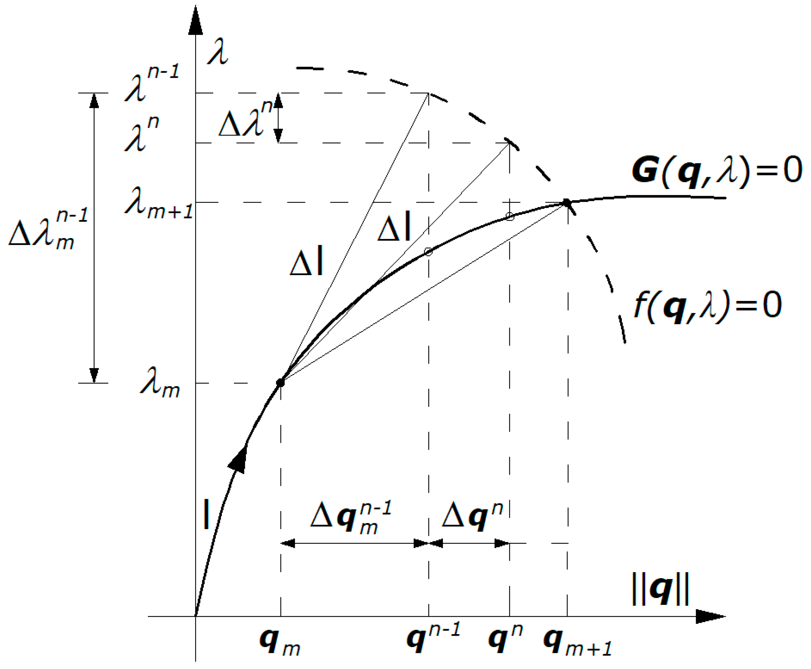
The constraints equation has the following form [25].
where is the increment (parameter) of the arc length on the solution path, is a vector of the searched displacements, is the increment of the current load parameter , is the increment of the current vector of unknown displacements in relation to the last convergent values of the load parameter and displacement vector , which were obtained with the assumed accuracy in the previous load step .
Directly solving the constraints Equation (31) allows for us to determine the load parameter . The solution requires checking the differentiator sing and was determined according to the following two equations.
and
Then, the solution is selected as the smallest “distance” away from the solution that was obtained in a previous load step . The smallest “distance” responds to the smallest angle (or the largest cosine of the angle) between the solutions in actual load step and the previous one :
Analyzing the conditions of the solution to the constraints Equation (31), indicates that this criterion can be described by the following equation.
This extended system can be solved using a two-stage procedure described below.
- Prediction stage —for known initial values established in the previous load step (i.e., , , ), the load parameter is determined using the constraints Equation (31):
- Correction stage —is realized in four iterative steps.
- (a)
- New displacement increments are determined using the system of motion Equations (7).
- (b)
- The load parameter is determined using Equation (13).
- (c)
- The updated displacements vector is calculated, according to: .
- (d)
- The iterations are terminated after reaching a predefined accuracy and then the load and displacement parameters are updated , and the next load step starts from a new prediction stage. If the predefined accuracy is not achieved, then the next correction stage is required.
On the basis of carried out numerical experiments, it was determined that the accuracy should satisfy .
Figure 7 shows the iterative scheme for solving the extended system of Equations (30).
5. Numerical Results
5.1. Reinforced Concrete Beam
To analyze the beam, the computational methods must be adapted to the specific behavior of a reinforced concrete bent element, with regard to the shear effect on its load-carrying capacity. To this end, the general system of Equations in (9) was reduced by omitting the influence of longitudinal forces on displacements of the beam, so that it can be used to describe moderately large displacements of the bar systems.
5.1.1. Experiment Details
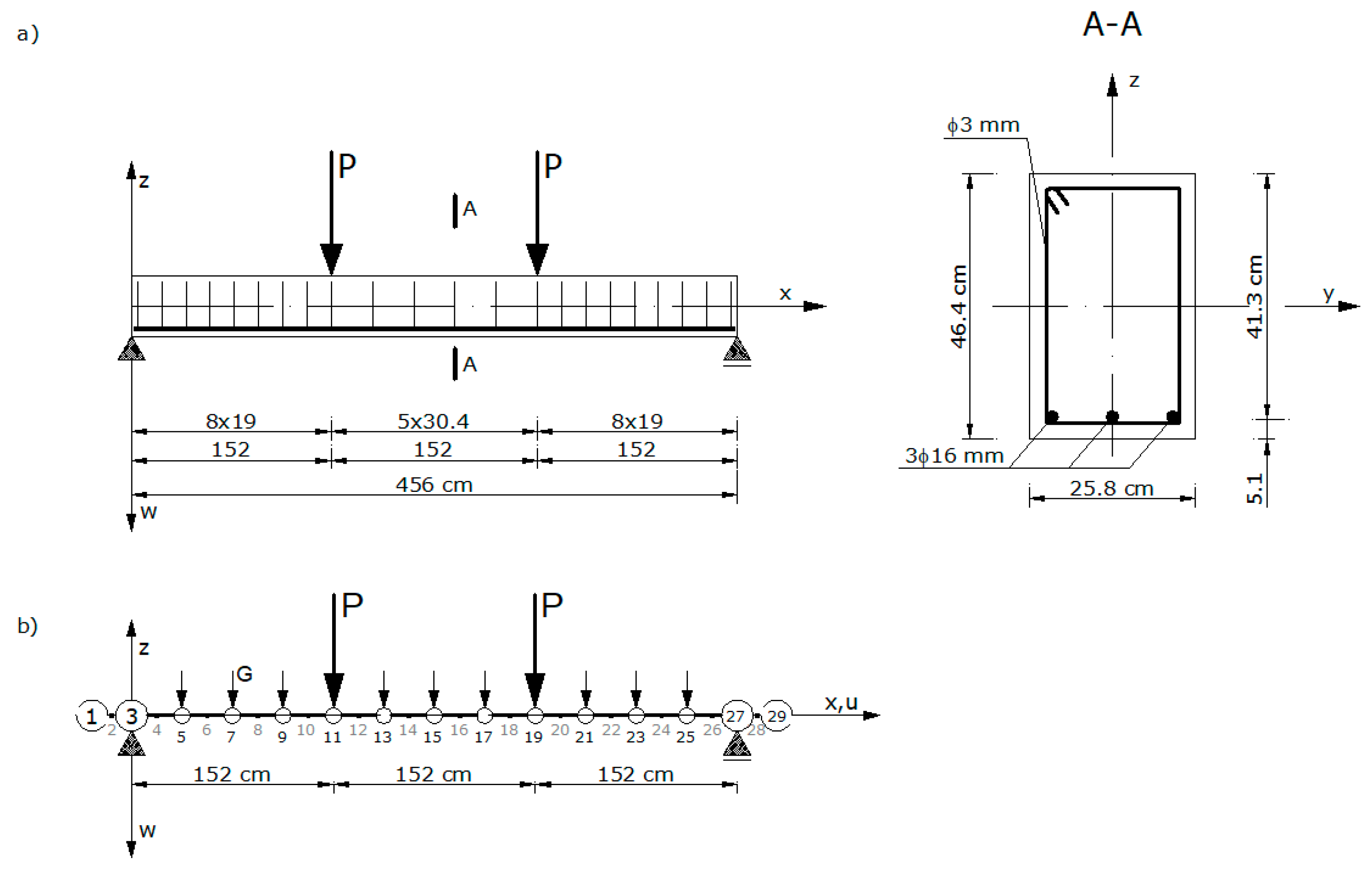
A C1 type beam was investigated and experimentally tested by Buckhouse [27,28]. A single-span, simply supported beam with a rectangular cross-section was analyzed. The load on the beam formed two concentrated forces. The static scheme of the beam is shown in Figure 8a. The beam is reinforced by three -mm bars, and the transverse reinforcement is from stirrups made with -mm bars.
The following material properties were used for concrete. The compressive strength was determined from experiments in [28]. Other material properties were determined in accordance with [34], as shown below. The tensile strength was , determined according to , where is expressed in . The shear strength was . The deformation modulus was determined according to where is expressed in . The limit strains were and and Poisson’s ratio was .
The following material properties were used for the reinforcing steel. These material properties were taken from Reference [28]. The yield stress for compression and tension was , the deformation modulus was , the limit strains were , and Poisson’s ratio was .
The density of the reinforced concrete was set to , the critical value of the damping factor for bending vibrations to , and the critical value of the damping factor for rotational vibrations to .
Discretization of the central axis of the C1 beam consisted of introducing 29 nodes, which is shown in Figure 8b. Among the 23 internal nodes, there were 11 main nodes (odd) and 12 intermediate nodes or segments (even). There were two main nodes on each edge (real and fictitious) and one intermediate node (fictitious).
An external load was applied to the beam in the form of two concentrated forces at the designated main nodes . The self-weight of the individual segments was represented by the concentrated forces, applied at the main nodes excluding the boundary nodes. That is , .
5.1.2. Analysis of the Load-Carrying Capacity and Displacement
Figure 9 presents the numerical results for the C1 beam using the dynamic relaxation method with the arc-length parameter (DRM + AL). These results were compared with experimental, theoretical, and numerical finite element method results that were taken from the literature. The diagram illustrates the transversal displacements in the mid-span of the C1 beam in node 15 as the load function. The solid line represents the results using the DRM + AL with limit the load value and displacement value . These results were compared to Buckhouse’s experimental results (double thin solid line), and the numerical results of Smarzewski [35] (dense dashed line), and Wolanski [36] (dotted line). The numerical results presented in Reference [35] by Smarzewski were made by combining the procedures of the finite elements method with the arc-length method using ANSYS. The basis of the numerical results that are presented in Equation [36] by Wolanski was developed using the calibration of the finite element model in ANSYS. The sparse, dashed line is the theoretical limit load-carrying capacity that is determined according to principles of the plasticity theory for bar elements.
where is the limit bending moment for the reinforced concrete cross-section, and is the distance from the support axis to the application point of force . The theoretical limit load-carrying capacity of the beam calculated in this way is .
These numerical results agree with Buckhouse’s experimental results. Buckhouse experimentally determined the limit displacement value . This displacement was achieved by the DRM + AL for load value , which agrees with the experimental results by more than 98%.
The arc-length method allowed for observing the limit points for the displacement load function. There is a local softening area in Figure 9, which characterizes a decrease in the load that is related to an increase in the displacement. This phenomenon has been observed in experiments when the first crack appears and when the cracking zone increases in size. After the reinforcing steel achieved a full plastic state, subsequent softening areas were also observed.
The observed nature of the changes in transverse displacements and rotations over time indicates that the proposed numerical method is stable for the pseudo-time step , which was determined using Equation (29).
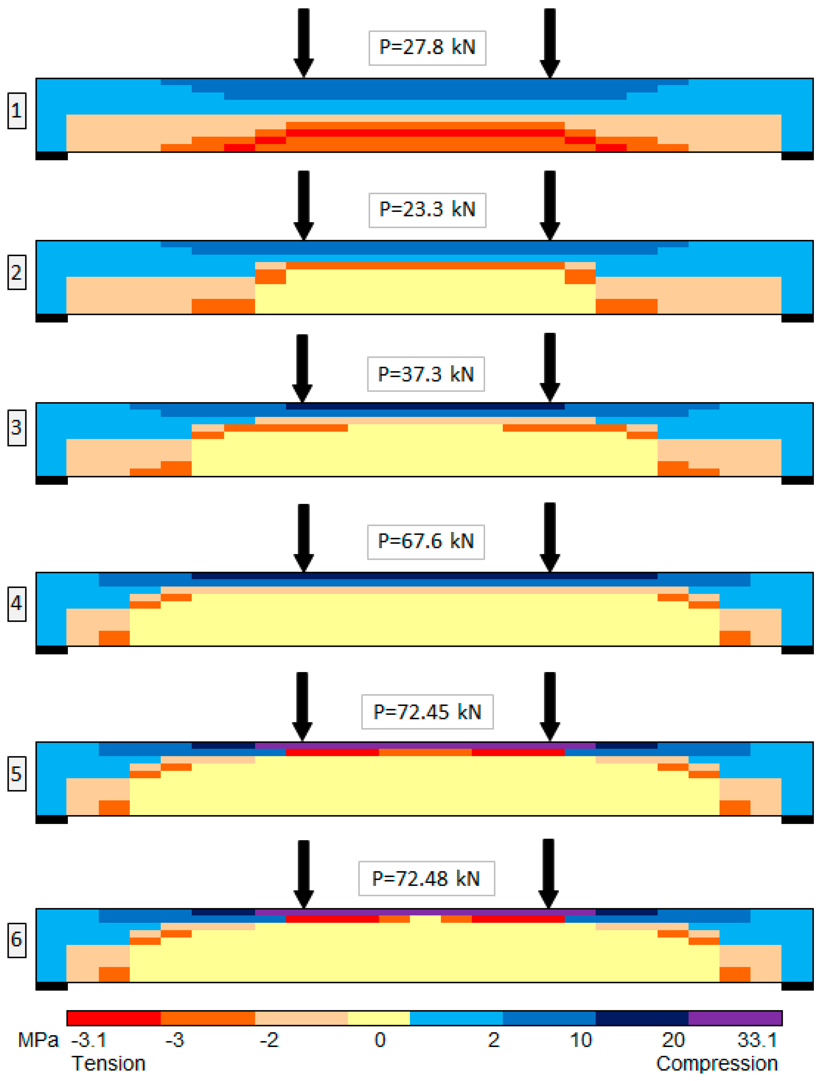
The stress state in subsequent effort steps of the C1 beam is presented in Figure 10. The load steps are marked by numbers |1|–|6| and correspond with the load steps that are indicated on the graph in Figure 9. The development of the element’s effort is observed from the elastic states |1| through the appearance of the first crack |2| to the plasticizing of the reinforcing steel |4| and the propagation of concrete softening processes |5| and |6|, in particular, areas of the structural element. The tracking of the stress state allows for a detailed description of the degradation in the critical cross-section leading to the destruction of the structural element.
5.2. Reinforced Concrete Column
A column was analyzed, taking into account the behavioral specifics of eccentrically compressed reinforced concrete elements. The general system of Equation (9) was reduced by omitting the influence of rotational inertial forces on displacements of the column. Consequently, the transverse force is treated as a passive force and the average non-dilatational strain angle is .
5.2.1. Experiment Details
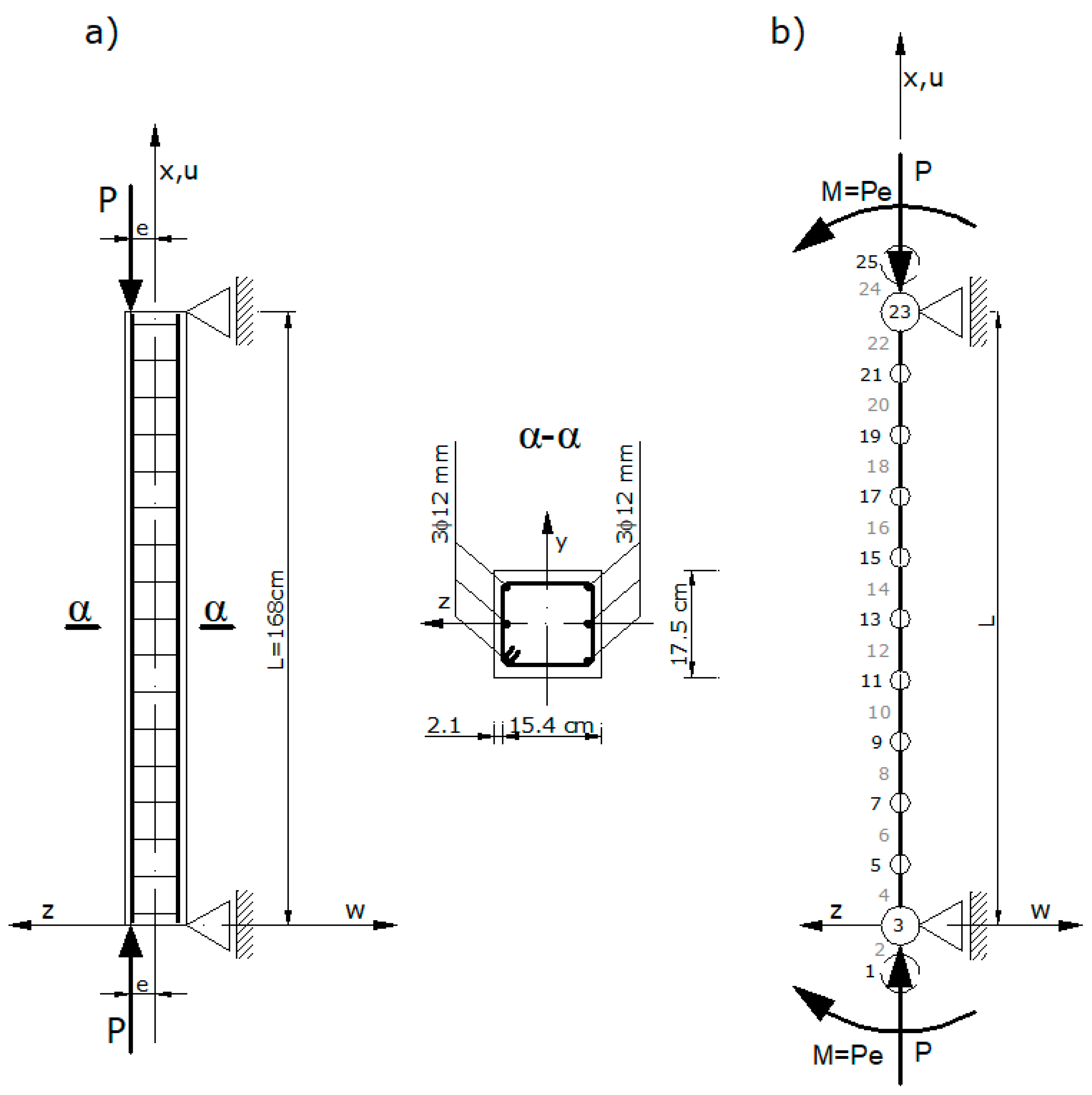
A numerical method was applied to the column that was investigated in experimental studies by Lloyd and Rangan [29], which they denoted as IB. The column was simply-sliding and supported in the longitudinal direction on both ends. Longitudinal forces were applied at the ends with a constant eccentricity , which is shown in Figure 11a. Analysis of columns loaded by longitudinal forces with other eccentricity values, such as and , were presented in the paper [37].
A column with constant dimensions and a square cross-section was analyzed. The column was doubly reinforced with three bars in each layer.
The discretization of the central axis produced 25 nodes, which is shown in Figure 11b. The internal division of the central axis of the column consists of 9 main nodes and 10 intermediate nodes (segments). There are two main nodes at the edges (one real and one fictitious) and one intermediate node (fictitious). The external load is interpreted as a longitudinal force and a bending moment , which was applied to the edge nodes
and , as shown in Figure 11b. The column was analyzed under the assumption that the force varies at constant eccentricity value .
The column was made of concrete with a compressive strength of . The concrete strength was determined on the basis of research that was conducted by Lloyd and Rangan [29]. They tested the cylindrical specimens and the results showed strengths of . Because , the specificity of high-strength concrete was considered according to the relationships developed by Collins et al. [38], when modeling the material behavior.
The following material properties were used for concrete. The compressive strength was , which was determined according to the strength-reducing criterion for the high-strength concrete proposed by Collins et al. [38]. The tensile strength was , which was determined by the relationship according to Reference [34], where is expressed in MPa. The deformation modulus was determined on the basis of Reference [38]. The strain limits values and were taken from Reference [31] and Poisson’s ratio was taken from Reference [34].
The following material properties were used for the reinforcing steel. These material properties were taken from Reference [29]. The yield stress in compression and tension was , the compressive and tensile strength (perfect plasticity) was , the deformation modulus was , the strain limit was , and Poisson’s ratio was .
5.2.2. Analysis of the Load-Carrying Capacity and Displacement
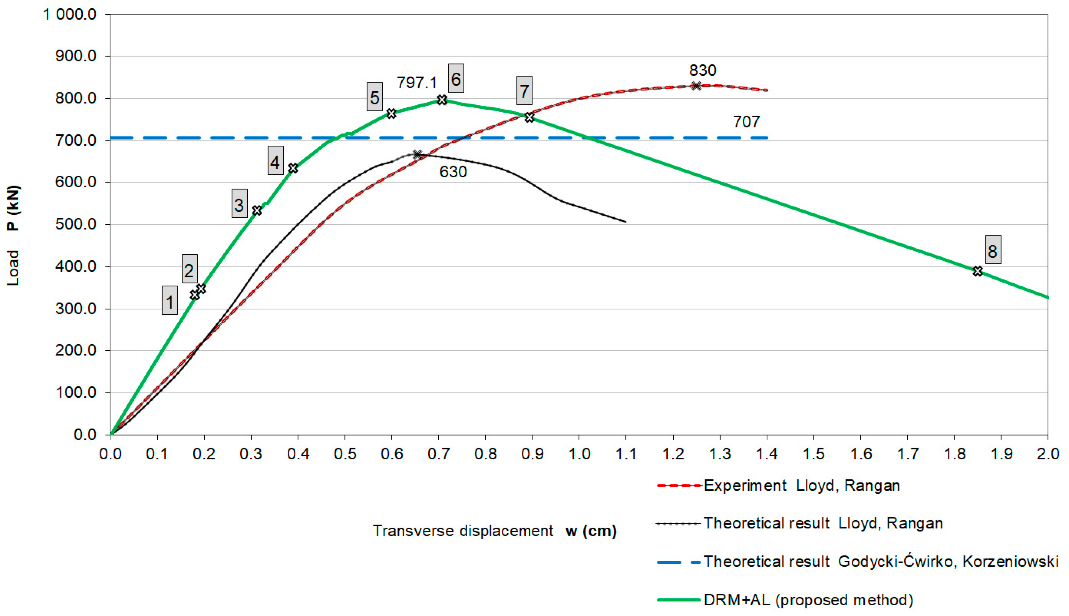
During the load-carrying capacity and displacement analysis, the results of numerical study for the IB column were compared with the experimental and theoretical results of Lloyd and Rangan [29], and the theoretical results of Godycki-Ćwirko and Korzeniowski [39]. The results for the load-carrying capacity were compared in terms of the cross-section displacement in the mid-span of the column, which can be seen in node 13.
Figure 12 shows the results for column IB. The results using the proposed DRM + AL are marked by the solid line.
The load-displacement diagram at node 13 using DRM + AL indicates the largest element stiffness among all of the cases that were considered. In this graph, small jumps in the displacements are observed for a load of . This represents the first crack in the tensile concrete layer for the middle cross-section of the column. Further developments in the cracking zone of the middle cross-section (and subsequent small jumps in the displacements) were observed at a load of . The load-carrying capacity, as determined by the numerical method, was , and the corresponding value for the transverse displacement was . The softening process in these three cases has similar characteristics. In the experimental analysis, the critical state was indicated at the highest load value of .
The DRM + AL results are the most similar to the experimental results, when compared with other methods. The load-carrying capacity of the column was 4% lower than the experimentally determined load and the displacement corresponding to the load-carrying capacity was 50% lower. The numerically determined load-carrying capacity of the column was 12% higher than the theoretical results of Godycki-Ćwirko and Korzeniowski [39]. The load-carrying capacity from the DRM + AL was 17% larger than Lloyd and Rangan’s results [29], while the displacement was 6% larger.
Moreover, the initial stiffens observed in numerical results obtained using DRM + AL differ from the experimental results. This effect is a consequence of the concrete modeling method and it is caused by adopting the idealized properties of structural material, especially the initial deformation modulus. The reduction of displacement values obtained by using DRM + AL is also related to the application of the overcritical damping value in the inelastic effort range of the structure.
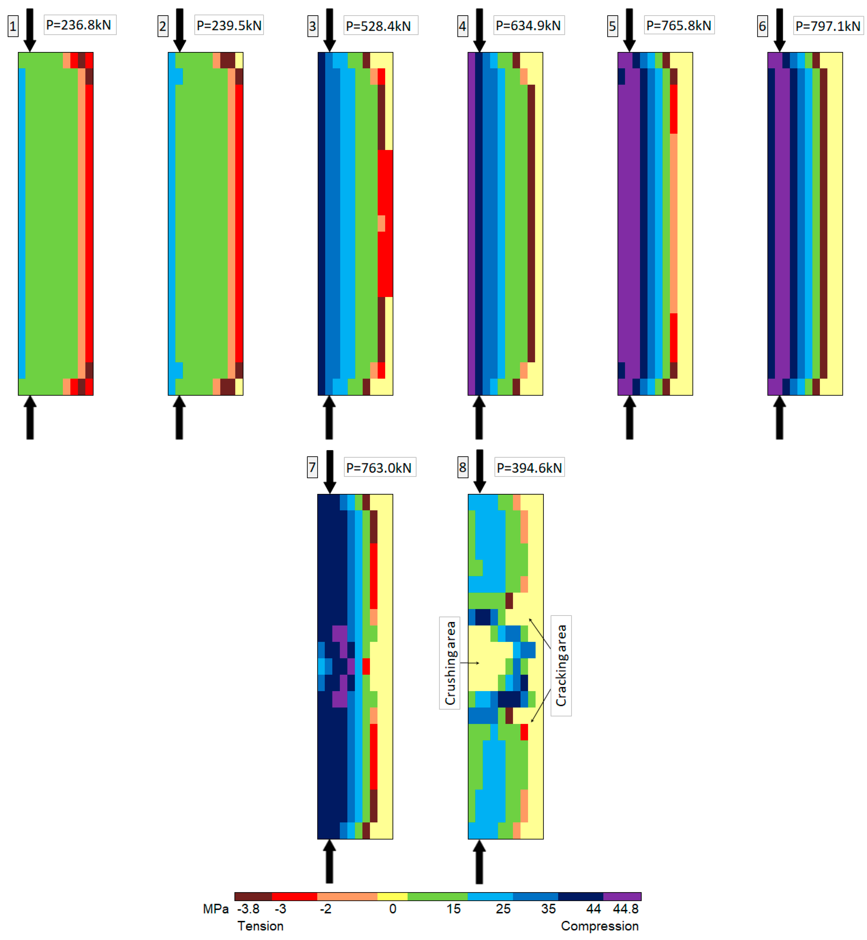
Figure 13 shows the stress state in subsequent effort steps of the IB column. The load steps are marked by numbers |1|–|8|and correspond with the load steps indicated in the graph of Figure 12. The first cracks in the tensile concrete layer occur in the cross-sections located near the edges of the column |2|. Further development of cracks propagates towards the center of the column |3–5|. Together with the increase of the load, it is observed that the plasticizing of the more compressed concrete external layer, which develops in an analogous manner to the development of the cracking process, i.e., progresses from the edge’s cross-sections towards the mid-span of the column. At the load value , the process of the concrete softening begins in the cross-sections that are located near the edges. The plasticizing area of the compressed concrete propagates into the internal layers of the cross-section, which is similar to the cracked area |5|. Reaching the limit value of the load capacity causes the development of the softening zones in the compressed concrete. Both the plasticizing zone in the compressed concrete and the cracked area in tensile concrete remains unchanged |6|. The development of the softening process among the cross-section causes the rearrangement of stresses and changes the direction of the degradation processes, which now develop in the center of the column and progress toward the support edges. In the post-critical range |7|, the advanced softening of the compressed concrete is observed together with the gradual development of plasticization zone in the mid-span sections of the column. The cracking area increases uniformly over the entire length of the column. The failure of the column occurs abruptly when the load is equal . The crushing concrete area concentrates in the mid-span of column and it covers half of the cross section height |8|. Previously cracked layers of cross-sections transfer the compressive stresses as a result of the cracks closing. Between crushed and cracked areas, there is still undamaged concrete, which is qualitatively compatible with the experimental results.
6. Conclusions
The paper presents a behavior analysis method for the bending and compression of reinforced concrete elements that are subjected to short-term static loads. The structural system analysis technique was developed using assumptions from the finite difference method. The central axis of the structural element was discretized, and the equilibrium equations and geometrical relationships in differential form were written. A joint-action rule was determined for the active concrete and steel layers of the discretized cross-sectional model.
A dynamic process that can describe the static problem by introducing critical damping, was analyzed. When this procedure is used to solve a system of nonlinear equilibrium equations it is referred to as the DRM. Using the DRM, the equations of motion can be recursively solved in subsequent pseudo-time instants for each node of the spatial division. There was no need to solve the system of algebraic equilibrium equations. The DRM was improved by introducing an additional constraint equation to the system of equilibrium equations based on the assumptions of the arc length method. This method is called the DRM + AL, and can be used to solve the nonlinear equilibrium equations in the post-critical range.
When modeling the behavior of structural materials, the reduced plane compressive/tensile states with shear stress was considered. Equations that were derived from the theory of moderately large displacements in a bar system form the basis of structural behavior description by assuming infinitesimal deformations. This assumption is appropriate when describing strain and stress states in the concrete and steel layers of commonly used reinforced concrete elements.
To verify the effectiveness of the developed method, numerical tests on a reinforced concrete beam and eccentrically loaded column, were carried out.
The reinforced concrete beam was analyzed in terms of its load-carrying capacity and displacement. The influences of isochoric deformations, and the shear and tensile strengths of concrete were considered. Numerical results described displacement changes with regard to the structural member in subsequent phases.
The comparative analysis, which was performed for reinforced concrete structural elements indicates that obtained numerical results agree with the experimental results. In case of a beam, numerically determined load carrying capacity is 3% lower than those that were determined in experiment. The load-carrying capacity of the column is 4% lower than the experimentally determined load, and the displacement corresponding to the load-carrying capacity was 50% lower. The results obtained using the dynamic relaxation method with the arc-length method are the most similar to the experimental results, when compared with the other analysis methods. For both of the structural elements, the proposed method enabled extensive analysis of the post critical effort.
The conclusions are summarized as follows.
- Comparative analysis of the results obtained for the bent and eccentrically compressed reinforced concrete elements indicate that the proposed method accurately estimated the load-carrying capacity.
- The considerations carried out and the obtained results of numerical analysis confirm the high efficiency of the developed computational method.
- The proposed method of dynamic relaxation taking into account the constraints equation for the non-linear equilibrium path enables the simulation of inelastic behavior of reinforced concrete elements in the range of continual formation for the failure mechanism.
- The numerical method is useful for tracking the global softening process of the structural element, in such that the range that cannot always be observed in the experiment because of the measurement limitations.
- A greater stiffness was observed in the computational model when compared with previously published experiments. This effect is a consequence of the concrete modeling method.
- In the inelastic range, there was a reduction in the displacement associated with the critical damping factor, which was determined using the longitudinal and flexural stiffness of the column in the elastic range.
- The computational method could be improved by further modifying the concrete model and by introducing a damping factor dependent on the inelastic state of the element. This would result in more precise estimates of the displacement.
- The proposed computational method is suitable for a post-critical analysis of the bending and eccentric compression of inelastic reinforced concrete elements.
- The proposed method is very useful for predicting the development of structural elements failure and for allowing a better analysis of the construction systems’ safety.
Acknowledgments
The research was supported by the Statutory Research Grant no 934 in the Faculty of Civil Engineering and Geodesy, Military University of Technology, Warsaw, Poland.
Author Contributions
Anna Szcześniak developed the computational method, computer program and performed numerical tests and wrote the manuscript. Adam Stolarski contributed to the idea of the study, modified the computational method, computer program and verified manuscript.
Conflicts of Interest
The authors declare no conflict of interest.
References
- Park, J.; Choi, J.; Jang, Y.; Park, S.-K.; Hong, S. An Experimental and Analytical Study on the Deflection Behavior of Precast Concrete Beams with Joints. Appl. Sci. 2017, 7, 1198. [Google Scholar] [CrossRef]
- Smarzewski, P.; Stolarski, A. Numerical Analysis on the High-Strength Concrete Beams Ultimate Behaviour. IOP Conf. Ser. Mater. Sci. Eng. 2017, 245. [Google Scholar] [CrossRef]
- Hao, T.; Cao, W.; Qiao, Q.; Liu, Y.; Zheng, W. Structural Performance of Composite Shear Walls under Compression. Appl. Sci. 2017, 7, 162. [Google Scholar] [CrossRef]
- Ye, J.; Jiang, L.; Wang, X. Seismic failure mechanism of reinforced cold-formed steel shear wall system based on structural vulnerability analysis. Appl. Sci. 2017, 7, 182. [Google Scholar] [CrossRef]
- Cichocki, K.; Domski, J.; Katzer, J.; Ruchwa, M. Impact resistant concrete elements with nonconventional reinforcement. Annu. Set Environ. Prot. 2014, 16, 1–99. [Google Scholar]
- Derysz, J.; Lewiński, P.M.; Wiȩch, P.P. New Concept of Composite Steel-reinforced Concrete Floor Slab in the Light of Computational Model and Experimental Research. Procedia Eng. 2017, 193, 168–175. [Google Scholar] [CrossRef]
- Szczecina, M.; Winnicki, A. Relaxation Time in CDP Model Used for Analyses of RC Structures. Procedia Eng. 2017, 193, 369–376. [Google Scholar] [CrossRef]
- Cichocki, K.; Ruchwa, M. Integrity analysis for multistorey buildings. Ovidius Univ. Ann. Ser. Civ. Eng. 2013, 15, 45–52. [Google Scholar]
- Siwiński, J.; Stolarski, A. Analysis of the dynamic behavior of a charge-transfer amplifier. In Dynamical Systems: Modeling; Springer Proceedings in Mathematics & Statistics; Springer: Berlin, Germany, 2015; pp. 341–352. [Google Scholar]
- Słowik, M.; Smarzewski, P. Study of the scale effect on diagonal crack propagation in concrete beams. Comput. Mater. Sci. 2012, 64, 216–220. [Google Scholar] [CrossRef]
- SŁowik, M.; Smarzewski, P. Numerical Modeling of Diagonal Cracks in Concrete Beams. Arch. Civ. Eng. 2014, 60, 307–322. [Google Scholar] [CrossRef]
- Tamayo, J.L.P.; Morsch, I.B.; Awruch, A.M. Static and dynamic analysis of reinforced concrete shells. Lat. Am. J. Solids Struct. 2013, 10, 1109–1134. [Google Scholar] [CrossRef]
- Nogueira, C.G.; Venturini, W.S.; Coda, H.B. Material and geometric nonlinear analysis of reinforced concrete frame structures considering the influence of shear strength complementary mechanisms. Lat. Am. J. Solids Struct. 2013, 10, 953–980. [Google Scholar] [CrossRef]
- Rodriguez, J.; Rio, G.; Cadou, J.M.; Troufflard, J. Numerical study of dynamic relaxation with kinetic damping applied to inflatable fabric structures with extensions for 3D solid element and non-linear behavior. Thin Walled Struct. 2011, 49, 1468–1474. [Google Scholar] [CrossRef]
- Hincz, K. Nonlinear Analysis of Cable Net Structures Suspended from Arches with Block and Tackle Suspension System, Taking into Account the Friction of the Pulleys. Int. J. Space Struct. 2009, 24, 143–152. [Google Scholar] [CrossRef]
- Bel Hadj Ali, N.; Sychterz, A.C.; Smith, I.F.C. A dynamic-relaxation formulation for analysis of cable structures with sliding-induced friction. Int. J. Solids Struct. 2017, 126–127, 240–251. [Google Scholar] [CrossRef]
- Rezaiee-Pajand, M.; Alamatian, J. The dynamic relaxation method using new formulation for fictious mass and damping. Struct. Eng. Mech. 2010, 34, 109–133. [Google Scholar] [CrossRef]
- Rezaiee-Pajand, M.; Sarafrazi, S.R. Nonlinear dynamic structural analysis using dynamic relaxation with zero damping. Comput. Struct. 2011, 89, 1274–1285. [Google Scholar] [CrossRef]
- Bel Hadj Ali, N.; Rhode-Barbarigos, L.; Smith, I.F.C. Analysis of clustered tensegrity structures using a modified dynamic relaxation algorithm. Int. J. Solids Struct. 2011, 48, 637–647. [Google Scholar] [CrossRef]
- Barnes, M.R.; Adriaenssens, S.; Krupka, M. A novel torsion/bending element for dynamic relaxation modeling. Comput. Struct. 2013, 119, 60–67. [Google Scholar] [CrossRef] [Green Version]
- De Borst, R.Ã.; Crisfield, M.A.; Remmers, J.J.C.; Verhoosel, C.V. Nonlinear Finite Element Analysis of Solids and Structures; Wiley Series in Computational Mechanics; Wiley: Hoboken, NJ, USA, 2012; ISBN 9781118376010. [Google Scholar]
- Pasqualino, I.P. Arc-length method for explicit dynamic relaxation. In Proceedings of the XXI International Congress of Theoretical and Applied Mechanics, Warsaw, Poland, 15–21 August 2004. SM1S-12607. [Google Scholar]
- Ramesh, G.; Krishnamoorthy, C.S. Post-buckling analysis of structures by dynamic relaxation. Int. J. Numer. Methods Eng. 1993, 36, 1339–1364. [Google Scholar] [CrossRef]
- Pasqualino, I.P.; Estefen, S.F. A nonlinear analysis of the buckle propagation problem in deepwater pipelines. Int. J. Solids Struct. 2001, 38, 8481–8502. [Google Scholar] [CrossRef]
- Wriggers, P. Nonlinear Finite Element Methods; Springer: Berlin/Heidelberg, Germany, 2008; ISBN 9783540710004. [Google Scholar]
- Lee, K.S.; Han, S.E.; Park, T. A simple explicit arc-length method using the dynamic relaxation method with kinetic damping. Comput. Struct. 2011, 89, 216–233. [Google Scholar] [CrossRef]
- Buckhouse, E.R. External Flexural Reinforcement of Existing Reinforced Concrete Beams Using Bolted Steel Channels; Marquette University: Milwaukee, WI, USA, 1997. [Google Scholar]
- Foley, C.M.; Buckhouse, E.R. Strengthening Existing Reinforced Concrete Beams for Flexure Using Bolted External Structural Steel Channels; Structural Engineering Report MUST-98-1; Marquette University: Milwaukee, WI, USA, 1998. [Google Scholar]
- Lloyd, N.A.; Rangan, B.V. Studies on High-Strength Concrete Columns under Eccentric Compression. Struct. J. 1996, 93, 631–638. [Google Scholar] [CrossRef]
- Stolarski, A. Model of dynamic deformation of concrete. Arch. Civ. Eng. 1991, 37, 405–447. [Google Scholar]
- Szcześniak, A.; Stolarski, A. A simplified model of concrete for analysis of reinforced concrete elements. Bull. Mil. Univ. Technol. 2016, 65, 55–68. [Google Scholar] [CrossRef]
- Alfarah, B.; López-Almansa, F.; Oller, S. New methodology for calculating damage variables evolution in Plastic Damage Model for RC structures. Eng. Struct. 2017, 132, 70–86. [Google Scholar] [CrossRef]
- Szcześniak, A.; Stolarski, A. Analysis of critical damping in dynamic relaxation method for reinforced concrete structural elements. In Proceedings of the Mathematical and Numerical Approaches, 13th International Conference Dynamical Systems—Theory and Applications, Lodz, Poland, 7–10 December 2015; Awrejcewicz, J., Kaźmierczak, M., Mrozowski, J., Olejnik, P., Eds.; ARSA Druk i Reklama: Łódź, Poland, 2015. [Google Scholar]
- EN 1992-1-1. Eurocode 2: Design of Concrete Structures—Part 1-1: General Rules and Rules for Buildings; Europea Commitiee for Standardization: Brussels, Belgium, 2004. [Google Scholar]
- Smarzewski, P. Numerical solution of reinforced concrete beam using arc-length method. Bull. Mil. Univ. Technol. 2016, 65, 33–46. [Google Scholar] [CrossRef]
- Wolanski, A.J. Flexural Behavior of Reinforced and Prestressed Concrete Beams Using Finite Element Analysis; Marquette University: Milwaukee, WI, USA, 2004. [Google Scholar]
- Szcześniak, A.; Stolarski, A. Numerical analysis of failure mechanism of eccentrically compressed reinforced concrete columns. In Insights and Innovations in Structural Engineering, Mechanics and Computation; Zingon, A., Ed.; Taylor & Francis Group: Cape Town, South Africa, 2016; pp. 1325–1330. [Google Scholar]
- Collins, M.P.; Macgregor, J.G.; Mitchell, D. Structural Design Considerations for High-Strength Concrete. Concr. Int. 1993, 15, 27–34. [Google Scholar]
- Godycki-Ćwirko, T.; Korzeniowski, P. Load-bearing capacity of HSC columns, estimated with use of simplified methods in the light of experimental results. Arch. Civ. Eng. 2000, 46, 39–49. [Google Scholar]
Figure 1.
Strength and stress parameters of the uniaxial tensile/compressive test for reinforcing steel.
Figure 1.
Strength and stress parameters of the uniaxial tensile/compressive test for reinforcing steel.

Figure 2.
Concrete model.
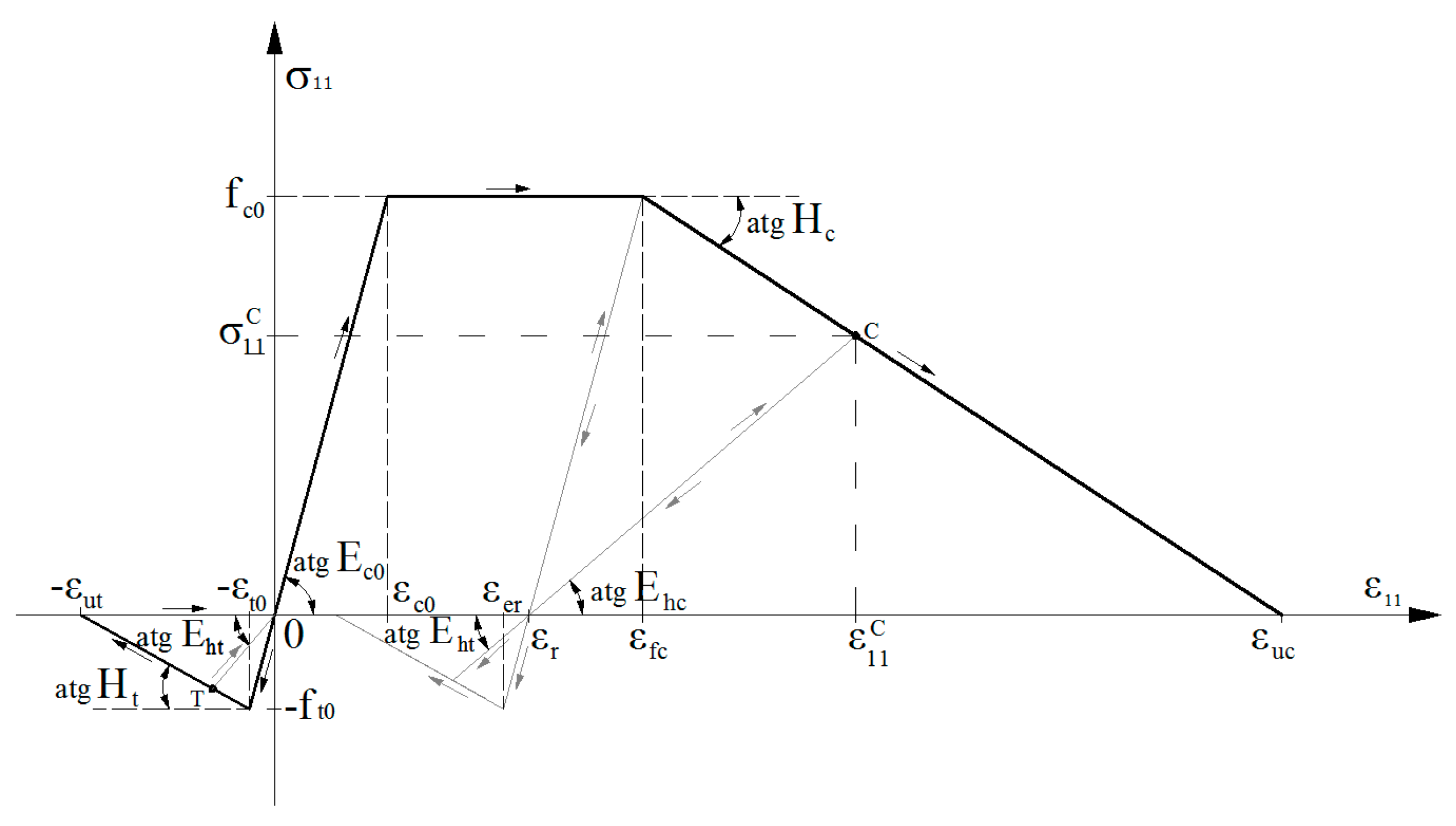
Figure 3.
Limit curve for the plane stress state.

Figure 4.
Equilibrium system of the internal forces.
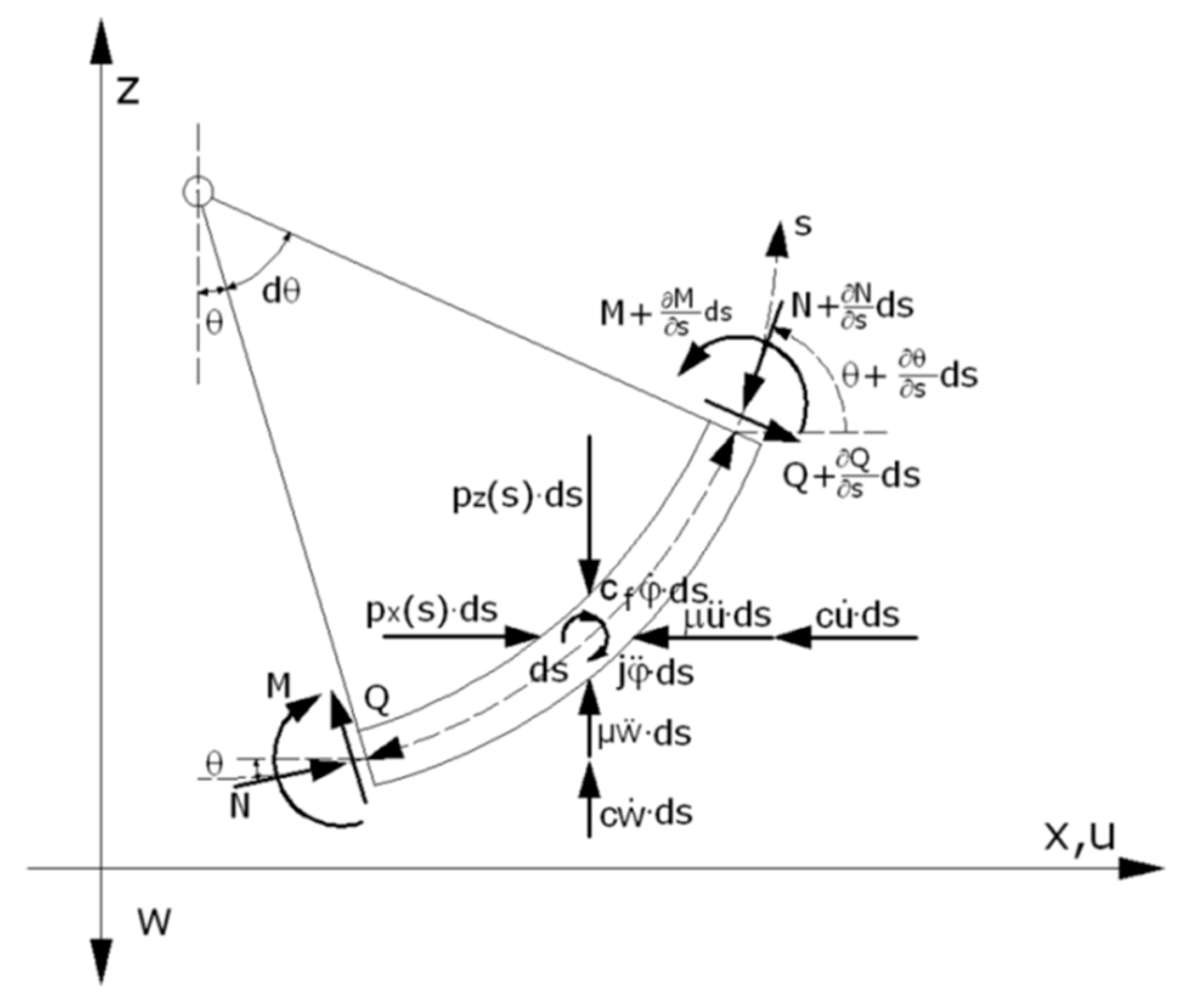
Figure 5.
Model of the reinforced concrete cross-section.
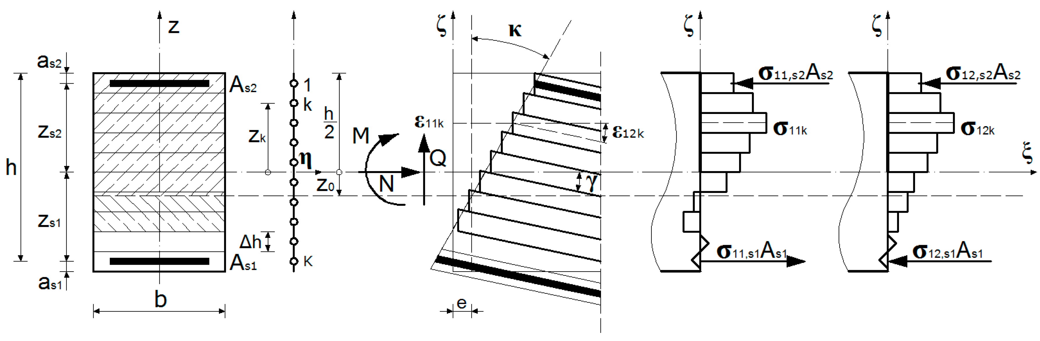
Figure 6.
Discretization of the bar’s structural element.
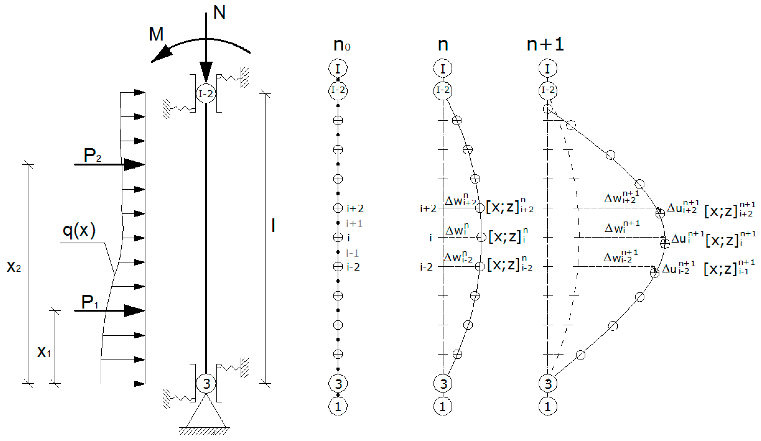
Figure 7.
Iterative scheme for solving the system of extended equations.

Figure 8.
Buckhouse’s C1 beam: (a) static scheme, (b) computational model.

Figure 9.
The numerical results using the proposed method for node 15 of the C1 beam compared with experimental and theoretical results from Buckhouse [27], Foley and Buckhouse [28], Smarzewski [35], and Wolanski [36].
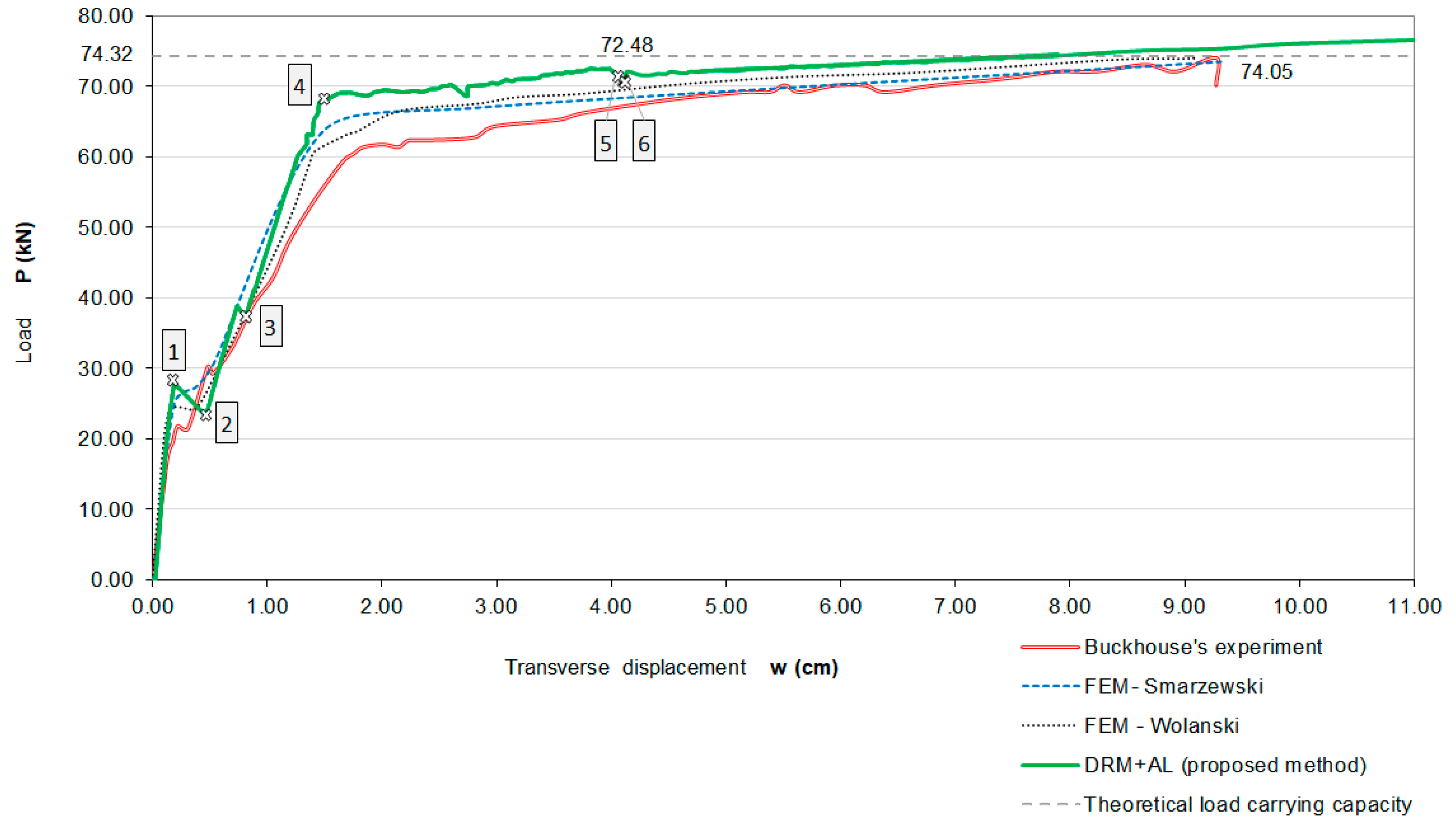
Figure 10.
Distribution of normal stresses depending on the load of C1 beam.

Figure 11.
The IB column, as presented in the paper [29]: (a) static scheme; (b) computational model of the column.
Figure 11.
The IB column, as presented in the paper [29]: (a) static scheme; (b) computational model of the column.

Figure 12.
Numerical results for node 13 of the IB column, compared with experimental and theoretical results from Lloyd and Rangan [29] and Godycki-Ćwirko and Korzeniowski [39].

Figure 13.
Distribution of normal stresses depending on the load of the column.

© 2018 by the authors. Licensee MDPI, Basel, Switzerland. This article is an open access article distributed under the terms and conditions of the Creative Commons Attribution (CC BY) license (http://creativecommons.org/licenses/by/4.0/).
Share and Cite
MDPI and ACS Style
Szcześniak, A.; Stolarski, A. Dynamic Relaxation Method for Load Capacity Analysis of Reinforced Concrete Elements. Appl. Sci. 2018, 8, 396. https://doi.org/10.3390/app8030396
AMA Style
Szcześniak A, Stolarski A. Dynamic Relaxation Method for Load Capacity Analysis of Reinforced Concrete Elements. Applied Sciences. 2018; 8(3):396. https://doi.org/10.3390/app8030396
Chicago/Turabian StyleSzcześniak, Anna, and Adam Stolarski. 2018. "Dynamic Relaxation Method for Load Capacity Analysis of Reinforced Concrete Elements" Applied Sciences 8, no. 3: 396. https://doi.org/10.3390/app8030396
Note that from the first issue of 2016, this journal uses article numbers instead of page numbers. See further details here.