An Innovative and Efficient Method for Reverse Design of Wheel-Rail Profiles
by
 , ,
, ,
Rong Chen
1,2 ,
,
Chenyang Hu
1,2,
Jingmang Xu
1,2,*,
Ping Wang
1,2,
Jiayin Chen
1,2 and
Yuan Gao
1,2 1
Key Laboratory of High-Speed Railway Engineering, Ministry of Education, Southwest Jiaotong University, Chengdu 610031, China
2
School of Civil Engineering, Southwest Jiaotong University, Chengdu 610031, China
*
Author to whom correspondence should be addressed.
Appl. Sci. 2018, 8(2), 239; https://doi.org/10.3390/app8020239
Submission received: 9 January 2018
/
Revised: 25 January 2018
/
Accepted: 31 January 2018
/
Published: 5 February 2018
Abstract
:Well-designed wheel-rail profiles are not only helpful in achieving expected dynamic vehicle performance but also in extending the service lives of wheels and rails. In this paper, a method for designing wheel-rail profiles is presented based on the rolling radius difference. This method consists of three parts, i.e., the reverse designs of wheel profiles, symmetric rail profiles and non-symmetric rail profiles. A reverse design method for wheel-rail profiles that can obtain smooth profile formed by quadratic curves is established according to the mapping relation between the rolling radius difference and the wheel-rail profile gradient. This reverse design method is verified and an example for optimizing the design of wheel profiles is introduced. Results show that the design method is effective and efficient. The static/dynamic indexes of the optimized wheel profiles matched with CHN60 can be greatly improved. According to the comparative analysis of wheel-rail contact and dynamic performance, when the lateral displacement reaches 6 mm, the maximum contact stress will be distributed evenly and can be decreased by 184.4 MPa compared to that of existing profiles, while the critical speed can be increased by 10.8% and the running stability can be improved by around 7%. It can be seen that this method is useful for the design of new wheel-rail profiles and optimization of existing wheel-rail profiles.
1. Introduction
The entire mass of the railway vehicle running on the track is borne by the wheels in contact with the rail and the vehicle is driven and guided by the traction and braking force created by wheel-rail adhesion. For railway vehicles, the proper design of wheel-rail profiles is helpful in achieving ideal vehicle operation, including curve negotiation, prevention of derailment, running stability and safety [1,2,3,4]. The design of wheel-rail profiles has been a topic of concern in many studies and many profile design methods with different targets and measures have been presented. Heller and Law [5] developed a design program for optimizing single arc wheel profiles. The different design requirements such as the wear characteristics, high critical speed or good curve negotiation could be satisfied by adjusting the radii of the wheel profiles. Smith and Kalouse [6] introduced a method for designing wheel-rail profiles of steering shaft vehicles. The required rolling radius difference could be satisfied by forming wheel-rail profiles with tangent arcs with different radii and two-point contact could be avoided. Leary and Handal [7] tried the instructive design of freight car wheel profiles based on expansions of rail shapes. Wu [8] designed subway wheel profiles based on the rail profile expansion method that are helpful in improving the compatibility of wheel-rail profiles, reducing the contact stress and finally reducing wheel-rail wear. Persson and Iwnicki [9] and Novales et al. [10] sought wheel profiles matching with the vehicle suspension parameters directly through dynamic simulation and the genetic algorithm and comprehensively analyzed the constraint conditions of different wheel-rail characteristics such as comfort, lateral track force, derailment coefficient, wear and contact stress. However, this method is very time-consuming. Shevtsov et al. [11,12] optimized the design of wheel profiles by taking the rolling radius difference as the design target according to multipoint approximation technology based on response surface fitting (MARS) and improved the profile matching and dynamic performance. Reference [13], based on the target functions and optimization method [11,12], optimized railway wheel profiles considering the wheel-rail rolling contact fatigue and wear etc. Jahed et al. [14] proposed a similar method to that used by Shevtsov et al. [11,12] and they chose a reduced set of generalized coordinates constituted by five variable parameters together with cubic spline curves in a linear programming formulation for the generation of profiles. The objective is to minimize the deviation of the rolling radii difference of the generated profiles from the target one. Polach [15] presented a method which established regardless of the roll angle for designing wheel profiles with target conicity and wide tread wear spreading by adjusting the estimated coefficient . Gerlici and Lack [16], based on the geometric characteristics shapes, developed railway wheel and rail head profiles by iteratively varying the arc radii profile variations. Igensti et al. [17,18] presented a wheel profile optimization method from the wear viewpoint and the method requires the contact point on rail, roll angle, optimization parameter k(y) and its range Ik. The rolling radius difference meets the design objective by adjusting the parameter k(y). The greater the resolution of Ik, the smaller the error but the longer the calculation time required and the range of Ik is too small to meet the design requirements and too large to increase the calculation time. Shen et al. [19,20,21,22] presented a method for designing wheel-rail profiles by taking the rolling radius difference or contact angle difference as design targets based on the wheel-rail contact geometric relation equation. Although the above methods each have their advantages, they cannot have high precision and high efficiency simultaneously.
This paper presents a reverse design method for wheel-rail profiles with the rolling radius difference as the target. The method consists of three parts, i.e., the wheel, symmetric rail and non-symmetric rail profile designs. Expected wheel profiles (rail profiles) can be designed based on given rail profile shapes (wheel profile shapes) and rolling radius difference curves and according to the dichotomy and loop iteration method. Compared with the above-mentioned methods, this is a reverse design method deduced from the mapping relation between a rolling radius difference and a wheel-rail profile gradient. According to this relationship, the wheel profile (rail profile) satisfying the target rolling radius difference can be obtained by adjusting the wheel profile (rail profile) gradients. In addition, with this relationship, we can better understand the effect of profile changes on the contact geometry. The designed wheel-rail profile formed by a multi-sectional quadratic curve can be directly output. Dichotomy is used during the numerical calculation in order to improve the calculation efficiency.
2. Geometric Analysis of Wheel-Rail Contact
2.1. Rolling Radius Difference
Figure 1 shows the schematic regarding geometric wheel-rail contact, where is the lateral wheelset displacement; is the rolling angle of the wheelset; is the left vertical minimum wheel-rail gap width; is the right vertical minimum wheel-rail gap width and ; is the rolling radius at the left wheel contact point; is the rolling radius at the wheel contact point when the wheelset is in a central position; is the rolling radius at the right wheel contact point.
Rolling radius difference:
where,
Figure 2 shows the right wheel-rail contact demonstrated using the wheel-rail profile gradient when the lateral wheelset displacement is , where the wheel profile is LMa which is widely used in China’s high-speed vehicle CRH2, the rail profile shape is CHN60 which is the 60 kg/m standard rail used in China, the rail gauge is 1435 mm and the rail cant is 1/40.
As shown in Figure 2, Line 1 indicates the rail gradient and Line 2 indicates the wheel profile gradient when and , the function of which is expressed by . Line 3 indicates the wheel profile gradient when and . Line 4 indicates the wheel profile gradient when and . Line 3 only considers the lateral wheelset displacement, namely moving by to the right based on Line 2. Line 4 considers the rolling angle, namely the wheel profile gradient increase based on Line 3 and a minor lateral displacement to the right.
Point a (the intersection point between Line 1 and 2) is the contact point on a wheel when and . Point d (the intersection point between Line 1 and 3) is the right wheel-rail contact point when and . Point e (the intersection point between Line 1 and 4) is the right wheel-rail contact point when and . Point b on Line 1 is the corresponding point of point d. Point c on Line 1 is the corresponding point of point e.
where , area refer to the value when and ; , area refer to the value when and ; refers to the rolling radius at the right wheel contact point when and ; refers to the rolling radius at the right wheel contact point when and and the rolling angle is considered; r0 refers to the rolling radius at the right wheel contact point without lateral displacement and rolling angle.
It is obvious that . The contact point at the right wheel when the rolling angle is considered is more biased towards the wheel flange side than when the rolling angle is neglected. The when the rolling angle is considered is higher than when the rolling angle is neglected.
The left wheel-rail contact under wheel-rail profile gradients can be described according to the above method. We can conclude that the contact point at the left wheel when the rolling angle is considered is farther from the flange side than when the rolling angle is neglected. The ΔrL. when the rolling angle is considered is higher than when the rolling angle is neglected.
According to the description of left/right contact, the geometric rule for wheel-rail contact is: the rolling radius difference obtained when the rolling angle is considered is higher than when the rolling angle is neglected.
2.2. Gradient Control
Two rules about slope control are given. The first rule is: taking the right wheel-rail as an example, when the rail profile does not change and the initial contact point and its right wheel profile gradient (>0) are given, the closer the left wheel profile gradient of the initial contact point is to the rail profile gradient, the higher the rolling radius difference will become; The second rule is: taking the right wheel-rail as an example, when the wheel profile does not change and the initial contact point and its right rail profile gradient are given, the closer the left rail profile gradient of the initial contact point is to the wheel profile gradient, the higher the rolling radius difference will become.
The first rule can be explained based on the following two points (the second rule can be explained in a similar way).
(1) Comparison between rolling radii differences, regardless of the rolling angle
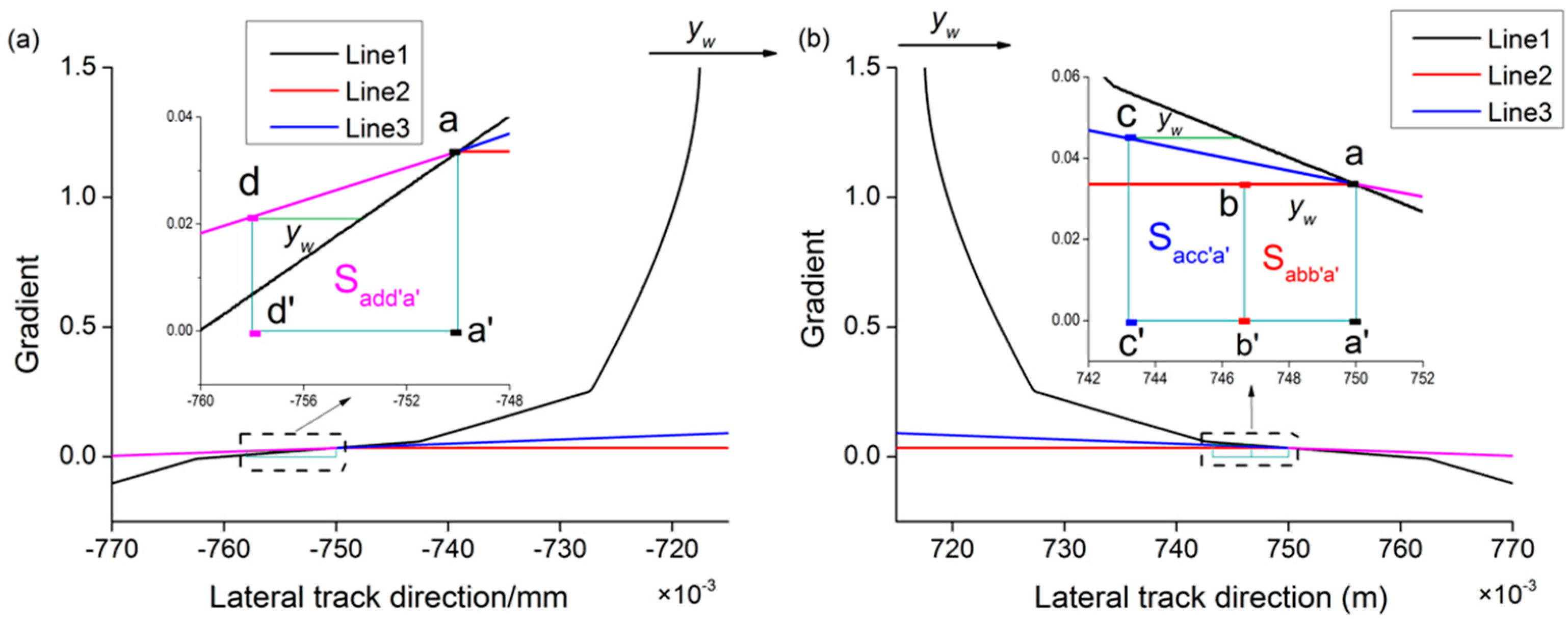
As shown in Figure 3, Line 1 indicates the rail profile gradient, Line 2 indicates a low wheel profile gradient and Line 3 indicates a high wheel profile gradient.
Left wheel-rail contact:
As shown in Figure 3a, the left wheel profile gradient (>0) of the initial contact point of Line 2 is equal to that of Line 3, so when the wheelset moves right laterally by yw, the left wheel-rail contact points of both wheels are the same. The ΔrL values for the left wheel-rail are the same.
Right wheel-rail contact:
As shown in Figure 3b, the wheel gradient of Line 3 is higher than that of Line 2. When the wheelset moves right laterally by yw, the wheel contact point of Line 3 is closer to the flange side compared with that of Line 2. The ΔrR value of Line 3 is higher than that of Line 2.
In summary, the rolling radius difference of corresponding wheels of Line 3 is higher than that of corresponding wheels of Line 2, without considering the rolling angle.
(2) Comparison between rolling radii differences, considering the rolling angle
When the rolling angle is considered, under the same lateral wheelset displacement, the corresponding wheel rolling angle of Line 3 is higher than that of Line 2.
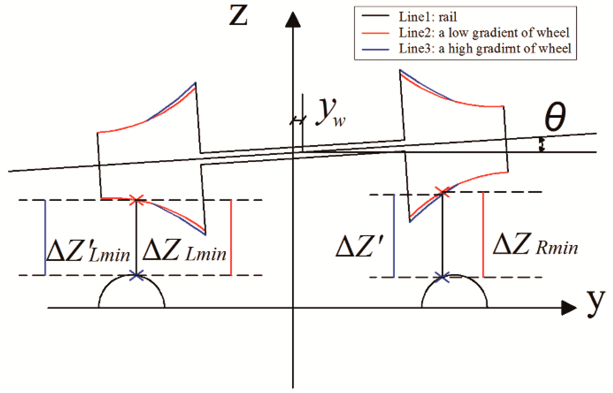
Figure 4 shows the geometric contact between the wheel of Line 2 and the rail. The lateral displacement is yw, the rolling angle is θ, the red intersection point is its wheel-rail contact point. is the minimum left wheel-rail gap, is the minimum right wheel-rail gap; at this time, . The profiles on the right (the side away from the flange) of the initial contact between the wheels of Lines 3 and 2 are the same. When the lateral wheel displacement and rolling angle of Line 3 are equal to those of Line 2, ( is the left minimum wheel-rail gap width for the wheel of Line 3). The wheel gradient of Line 3 on the left of the initial contact point is higher than that of Line 2 and (, is the right minimum wheel-rail gap width for the wheel of Line 3), so . The wheel of Line 3 needs a higher rolling angle in order to allow the vertical minimum wheel-rail gap width on the left to be equal to that on the right. Therefore, the wheel rolling angle of Line 3 is higher than that of Line 2.
When the rolling angle is considered, the corresponding wheel rolling angle of Line 3 is higher than that of Line 2. It can be ascertained from the geometric wheel-rail contact performance on gradients that the wheel ΔrR and of Line 3 is higher than that of Line 2.
Δr comparison: the wheel ΔrR and ΔrL of Line 3 are higher than those of Line 2, namely the closer the wheel gradient is to the rail gradient, the higher the rolling radius will become.
Applying this rule to reverse design of the wheel profile, the rolling radius difference can satisfy the target value through adjusting the wheel profile gradients. The rail profile can be created in the similar way like the wheel profile is created.
3. Reverse Profile Design Method
Reverse profile design comprises three parts: reverse design of wheel profiles, reverse design of symmetric rail profiles and reverse design of non-symmetric rail profiles. The three methods for designing profiles are similar; the following shows the reverse design of wheel profiles for reference.
A reverse design model for wheel profiles can be established based on the given rolling radius difference, initial wheel-rail contact point and its wheel profile shape away from the flange side (the wheel profile gradient is greater than 0). The initial wheel-rail contact point and its wheel profile shape away from the flange side are adopted herein for constraining the profile at one side, thus the designed wheel profile can meet the requirement through adjusting the profile of the other side.
3.1. Postulated Conditions
- (1)
- The wheel and rail are both rigid bodies and the wheel-rail contact is single point contact;
- (2)
- Convex rail head, namely the tangent gradient of each point varies monotonously;
- (3)
- The given rolling radius difference increases monotonously with the wheelset lateral displacement.
3.2. Method Description
The left- and right-side wheel profile and rail profile shape are symmetric, only the positive lateral displacement (lateral wheelset movement to the right) must be considered. The lateral displacement can be divided into n parts by a certain step length, which is expressed by (k = 1, 2, …, n). When the lateral displacement varies, the target value of the corresponding rolling radius difference will be .
Target function:
where refers to the target rolling radius difference when the lateral displacement is ywk; refers to the rolling radius difference of wheel profiles reverse designed when the lateral displacement is ywk.
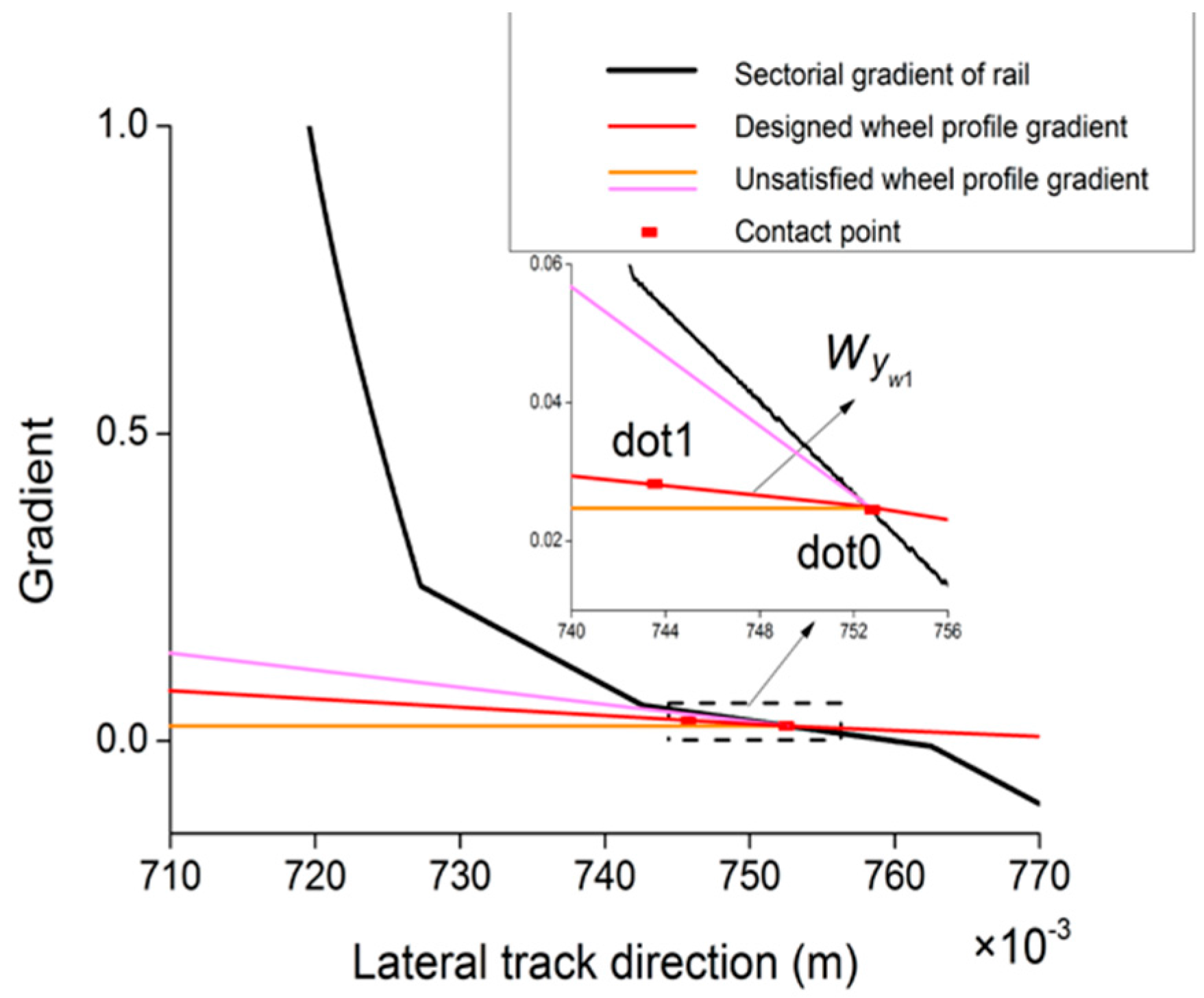
As shown in Figure 5, is the wheel profile gradient section and is the contact point on wheel when the lateral displacement is . In order to ensure that the curve of the designed wheel profile is smooth, the wheel profile gradients must be continuous and the wheel profile gradients of the designed sections must decrease monotonously. The gradients between contact points of the wheel profile in this design are straight lines. The profiles of the designed sections are multi-sectional quadratic curves. When the contact section gradients of the wheel profile are higher than 0, along with the wheelset moving right laterally, the contact points on the right wheel approach the flange side and the contact points on the left wheel leave the flange side gradually, enabling design of the wheel sections. As shown in Figure 6, the wheel profile gradient section satisfying the target function when the lateral displacement is is calculated first, then the wheel profile is found that satisfies the requirements by adjusting the wheel profile gradient on the left of the initial contact point until the target function of the designed profile shape satisfies the requirements. The contact point on the wheel under this lateral displacement is then chosen and finally the wheel profile gradient section . In a similar way, the wheel profile gradient section is calculated satisfying the target function by adjusting the wheel profile gradient on the left of the contact point when the lateral displacement is , until the target function satisfies the requirement when the maximum lateral displacement is ywn and then the completed designed wheel profile is output.
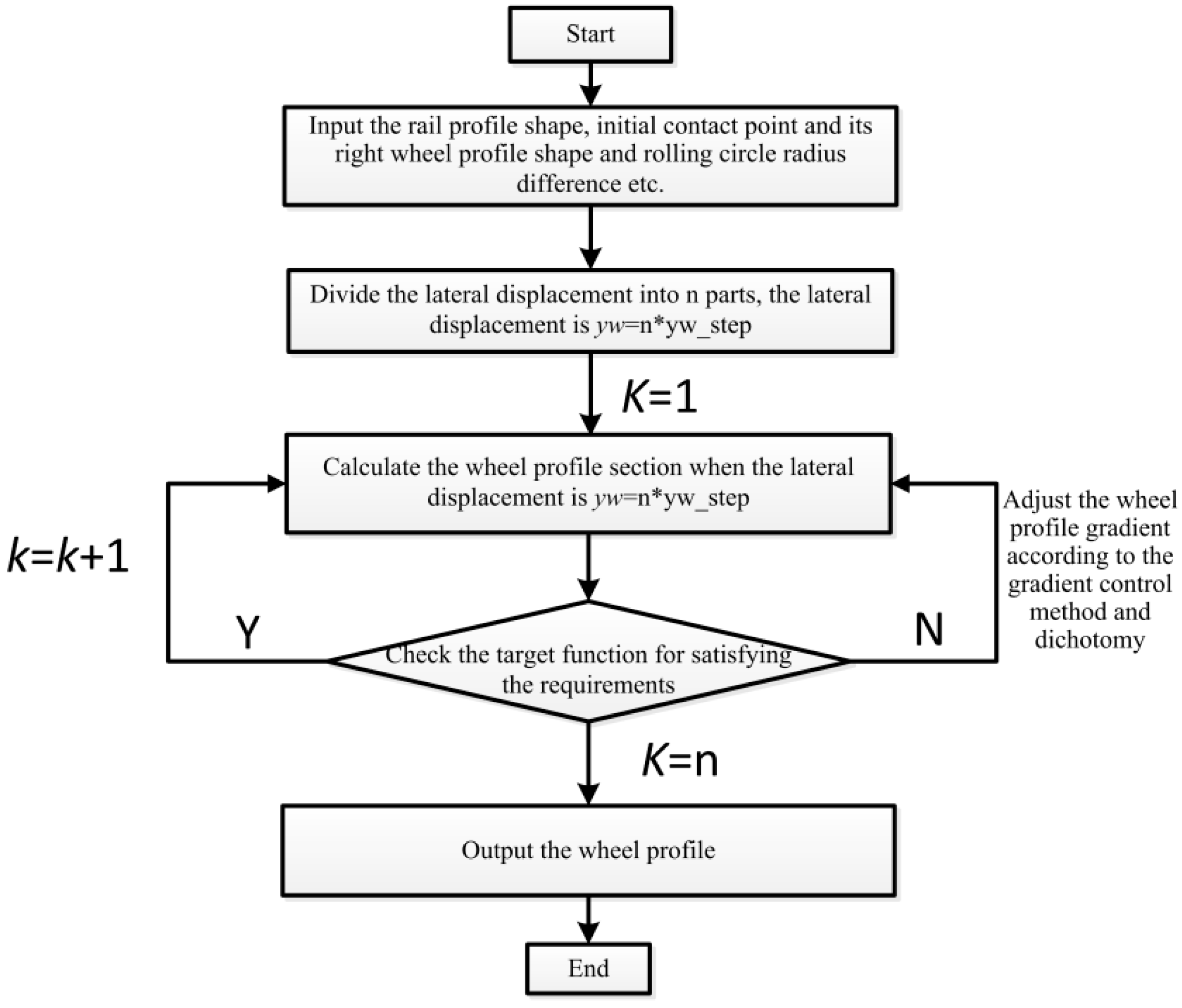
When the wheel profile gradient on the left of the initial contact point is low, the rolling radius difference corresponding to the wheel profile will be less than the target value. However, when the wheel profile shape gradient on the left of the initial contact point is high, the rolling radius difference corresponding to the wheel profile will be higher than the target value; therefore, dichotomy can be adopted to adjust the wheel profile gradient of designed sections. Using dichotomies can quickly converge to the target. Figure 7 shows the program flowchart.
4. Method Verification
4.1. Design of Wheel Profile
The effectiveness of the design method is illustrated by reverse design of the existing wheel profile. The wheel profile shape is designed in reverse by taking the rolling radius difference between the LMa wheel profile and CHN60 rail as the target. The rail gauge is 1435 mm, the nominal rolling radius is 430 mm and the rail cant is 1/40.
- (1)
- The profile shape of the CHN60 rail is given;
- (2)
- The initial given contact point is the same as that of LMa and CHN60 rail;
- (3)
- The LMa wheel profile shape on the right of the initial contact point is given.
The profile designed in reverse is checked for conformity with the LMa profile in order to verify the correctness of the design.
4.2. Design of Symmetric Rail Profiles
The effectiveness of the design method is illustrated by reverse design of the existing symmetric rail profile. The rail profile shape is designed in reverse by taking the rolling radius difference between the LMa wheel profile and CHN60 rail as the target. The rail gauge is 1435 mm, the nominal rolling radius is 430 mm and the rail cant is 1/40.
- (1)
- The LMa wheel profile is given;
- (2)
- The given initial contact point is the same as that of LMa and CHN60 rail;
- (3)
- The CHN60 rail profile shape on the right of the initial contact point is given.
The profile designed in reverse is checked for conformity with the CHN60 profile shape in order to verify the correctness of the design.
4.3. Designed of Non-Symmetric Rail Profiles
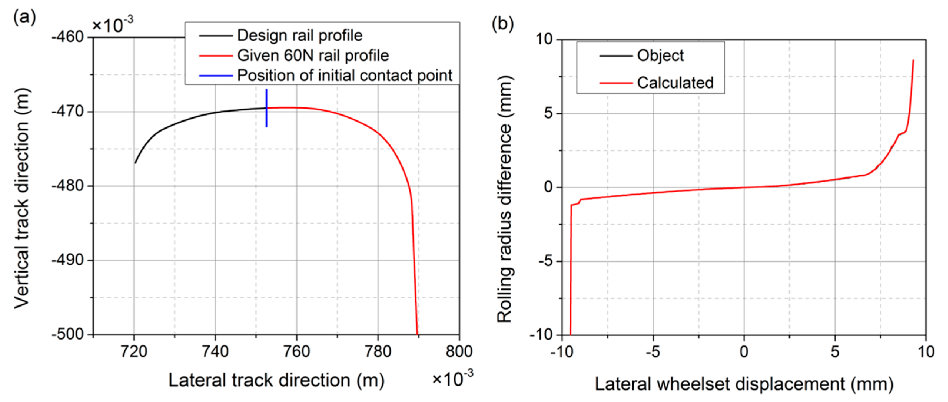
The effectiveness of the design method is illustrated by reverse design of non-symmetric rail profile. The rail profile shape is reverse designed by taking the non-symmetric rolling radius difference as the target (the negative part of the lateral displacement is the rolling radius difference when 60 N rail profile matches LMa; the positive part of the lateral displacement is the rolling radius difference when CHN60 matches LMa). The rail gauge is 1435 mm, the nominal rolling radius is 430 mm and the rail cant is 1/40.
- (1)
- The LMa wheel profile is given;
- (2)
- The left rail profile is given (60 N rail profile);
- (3)
- The 60 N rail profile shape on the right of the initial contact point is given.
The rolling radius difference designed in reverse is checked for conformity with the given one in order to verify the correctness of the design.
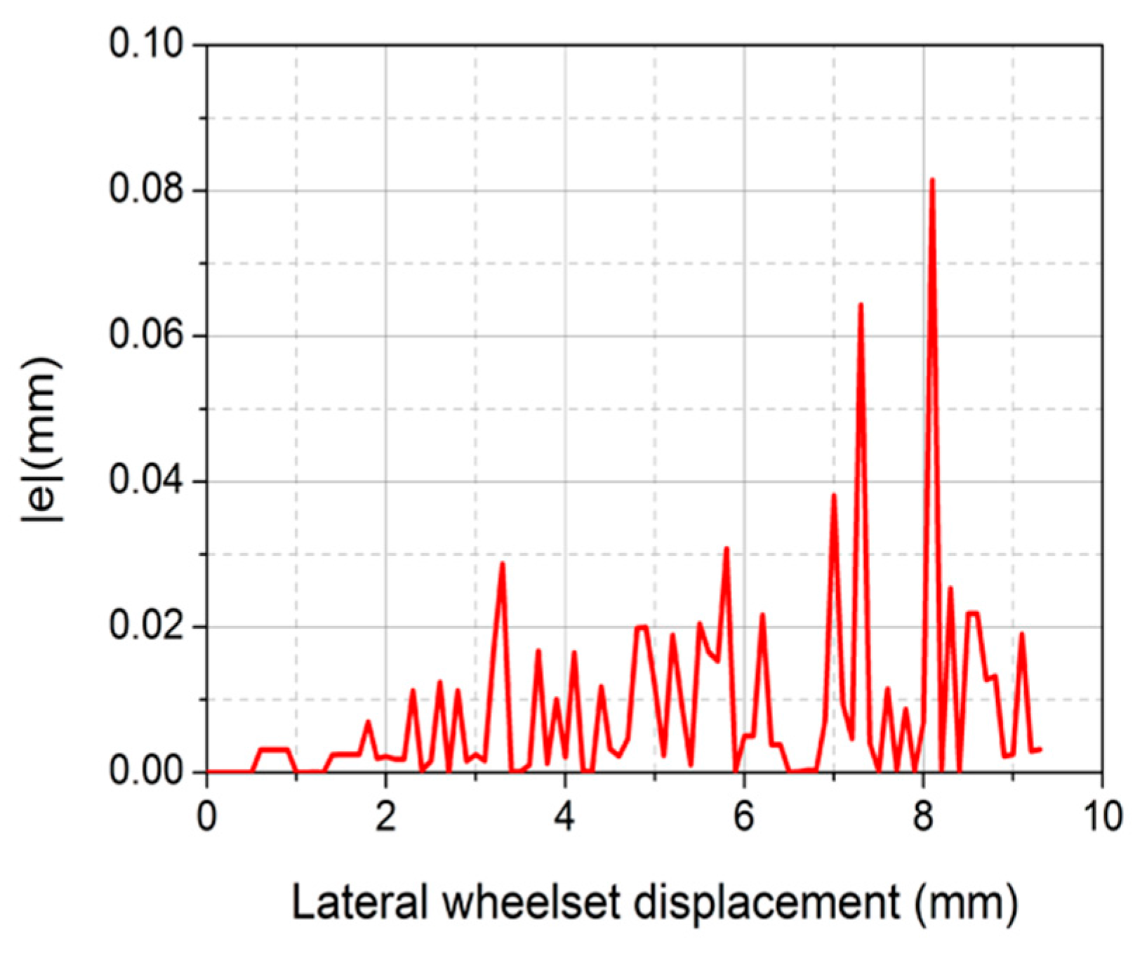
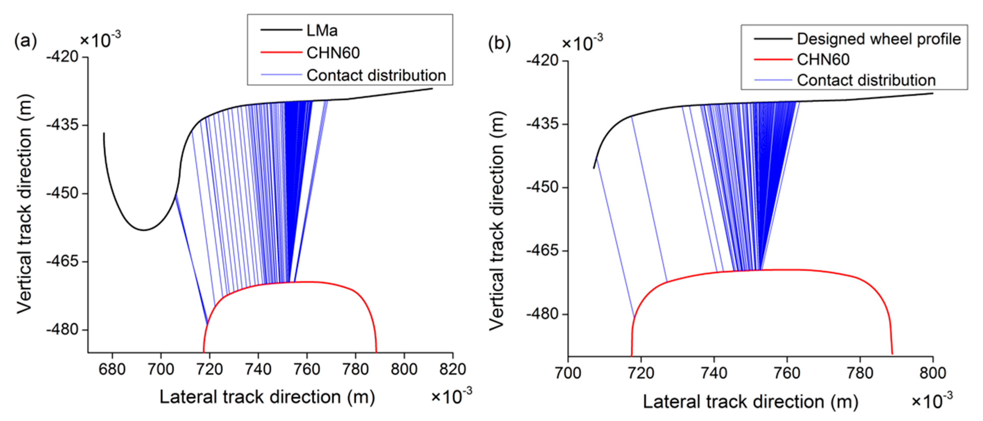
The new rail profile is shown in Figure 12a and the rolling radius difference is compared with the original one in Figure 12b; it shows that the two plots are almost coincident and that the error (see Figure 13) is about zero. Figure 14 shows the distribution of wheel-rail contact pairs. The rolling radius difference at the positive part of the lateral displacement is high and the distribution of contact points is wide.
Through the calculation of the above three examples, the calculation time is about 7.2 s and the physical memory (RAM) used is about 4110 MB.
5. Application Example
The new designed wheel profile aims to guarantee the kinematic characteristics of the original matching formed by LMa wheel profile and 60 N rail profile, also with the new designed wheel profile–CHN60 rail profile. The original matching has been chosen because it is characterized by good performances in kinematic behavior and CHN60 rail profile is widely common in China railways.
A wheel profile matching a CHN60 rail is reverse designed by taking the rolling radius difference between the LMa wheel profile and 60 N rail as the target. The rail gauge is 1435 mm, the nominal rolling radius is 430 mm and the rail cant is 1/40.
- (1)
- The CHN60 rail profile shape is given;
- (2)
- The initial contact point is given;
- (3)
- The LMa wheel profile shape on the right of the initial contact point is given.
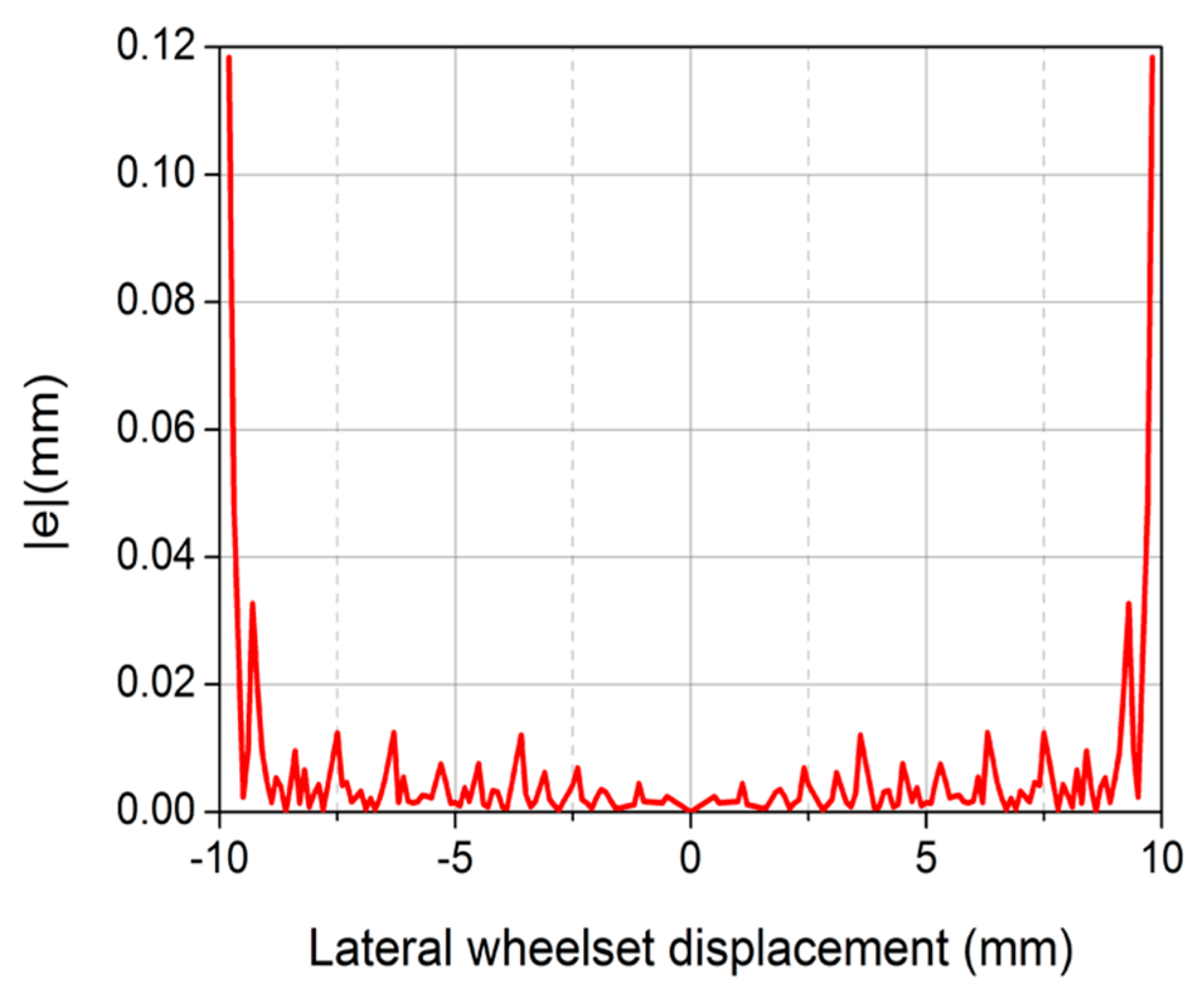
Figure 15a shows the comparison between the optimized wheel profile and LMa profile. The rolling radius difference is compared with the original one in Figure 15b; it shows that the two plots are almost coincident and that the error (see Figure 16) is about zero. Figure 17 shows the contact pairs of the optimized wheel profile. The lateral displacement is within −9.8 mm–9.8 mm, the lateral displacement space is 0.2 mm. The contact for the optimized wheel profile is more intensive.
5.1. Contact Bandwidth
In order to accurately characterize the hunting movement of wheelset, the horizontal ordinate variation range of wheel profile contact points at one side when a wheelset moves to the positive/negative direction under a certain lateral displacement is defined as a contact bandwidth. The ratio of the contact bandwidth to the lateral wheelset displacement range is adopted as the contact bandwidth ratio. The contact bandwidth and its ratio indexes reflect the variation of contact points along the axial direction of the wheelset.
Figure 18 shows the contact bandwidth and contact bandwidth ratio when the two types of wheel profiles match a CHN60 rail. It can be seen that when no flange contact occurs, both the contact bandwidths and contact bandwidth ratios of LMa and optimized wheels increase with the increase of the lateral wheelset displacement and the contact bandwidth and contact bandwidth ratio of the optimized wheel are less than those of the LMa profile, indicating that the vehicle runs most stably when the optimized wheel profile matches the CHN60 rail, however the wheels and rail are liable to fatigue and damage due to regular contact at the same position.
5.2. Wheel-Rail Contact Stress and Contact Patch Distribution
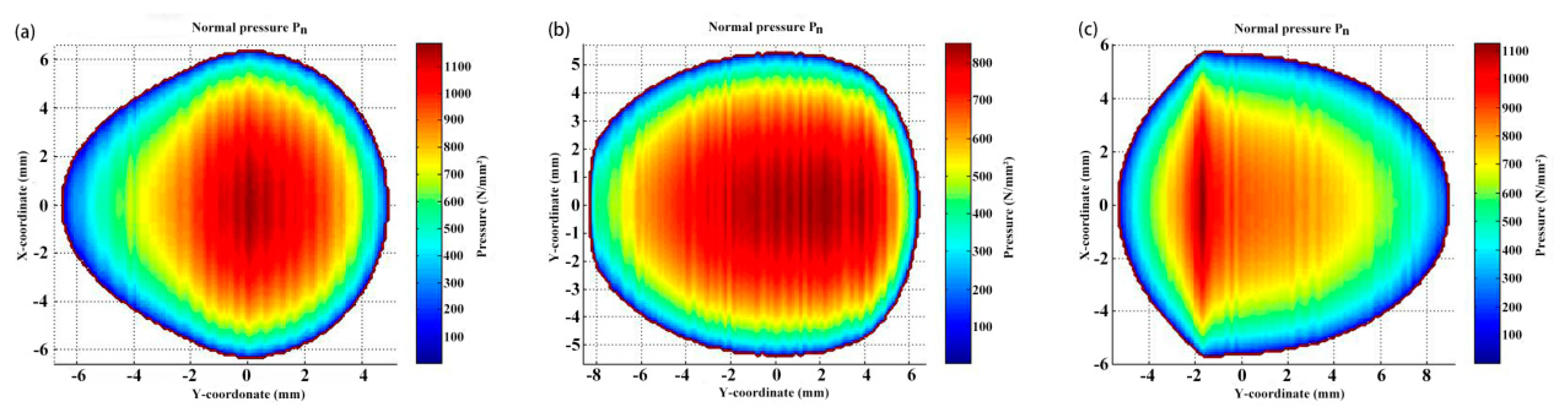
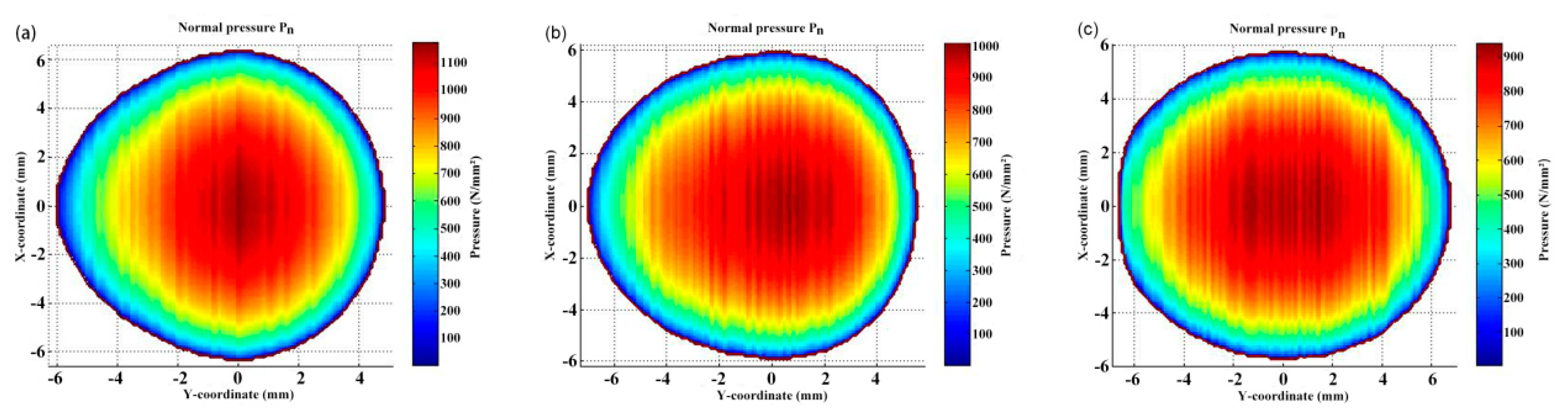
The wheel-rail contact patch shape and contact stress distribution when different wheel and rail profiles match are described by taking the lateral wheelset displacements of 0 mm, 3 mm and 6 mm as the examples. Figure 19 and Figure 20 show the distribution of contact stress when different wheel and rail profiles match; for the comparison of maxima, see Table 1.
As shown in Figure 19 and Figure 20, the contact patch shapes on the rail do not demonstrate much difference when the lateral wheelset displacement is 0 mm and 3 mm but differ obviously when the lateral wheelset displacement is 6 mm. This is mainly dependent on the corresponding wheel-rail contact geometry, showing wheel-rail matching is crucial to the contact pressure. Figure 21 shows the maximum wheel-rail contact stress at different wheelset displacement.
As shown in Table 1, when the lateral displacement is 0 mm, the contact patch shapes and areas do not change much and the maximum contact stress values are close to each other. When the lateral displacement is 3 mm, the contact patch shapes do not change much, the contact patch areas are large when CHN60 matches LMa and the degree of concentration of maximum compressive stresses is low. When the lateral displacement is 6 mm, the contact patch shapes are dumbbell-like when CHN60 matches LMa and the degree of concentration of maximum compressive stresses is high, because the wheel-rail contact points are dispersed and the contact bandwidths are wide. The contact patches are round when CHN60 matches optimized wheels and the degree of concentration of maximum compressive stresses is low, because the wheel-rail contact points are concentrated and the contact bandwidths are narrow.
5.3. Dynamic Performance Analysis
In this paper, a dynamic vehicle-track simulation model is established based on the Simpack multi-body dynamic simulation software, where the vehicle parameters of high-speed multiple unit (MU) CRH2 are adopted for the vehicle model. As shown in Reference [23], according to their structural characteristics, high-speed bogies without considering side bearing, swing bolsters and swing platforms are used in order to establish a four-axle locomotive dynamic model. During the establishment of the model, the main structural components of the vehicle are simplified as rigid bodies, including the wheelset, bogie and vehicle body etc. The secondary suspension between the vehicle body and two bogies and the primary suspension between the two bogies and four wheelsets are simulated with springs and damping elements. Each suspension point has three degrees of freedom (DOF, longitudinal, lateral and vertical degree of freedom). The main motion mode of the wheelset is rolling, so except for the dive motion of the four wheelset rigid bodies, 5 DOFs with regard to lateral displacement, side rolling, up-and-down, dive and yaw are considered. Thus, there are 7 rigid bodies and 31 DOFs to consider with regard to the whole vehicle model.
The dynamic performance of CHN60 rail profiles, optimized wheel profiles and LMa wheel profiles are compared based on three points i.e., the nonlinear critical vehicle speed, vehicle running stability and curve negotiation capability.
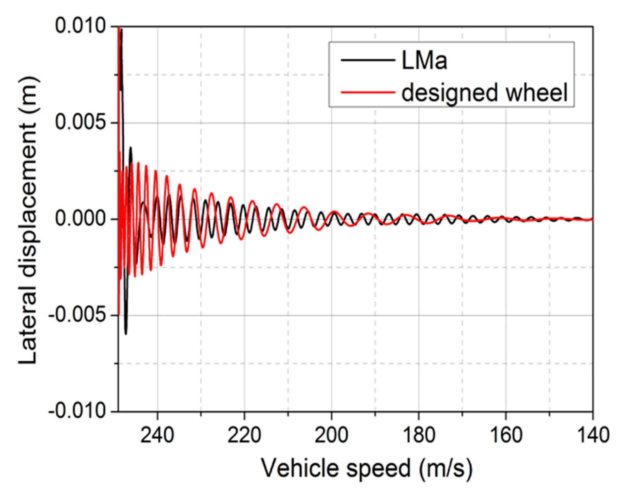
(1) Critical speed
Critical speed is the basic parameter for measuring the running stability of high-speed trains. In this paper, the nonlinear critical speed of high-speed EMUs is calculated based on the time domain response method. First, a section of irregularity is exerted at random on a track in order to excite the vibration of the vehicle system and then the speed of the vehicle on this track is reduced at a certain deceleration and the lateral wheel-rail displacement is observed for convergence to judge its critical speed. When the lateral wheelset displacement is less than 0.1 mm, it can be considered convergent and the corresponding speed at this time can be considered the critical speed of the train.
Figure 22 shows the simulated results. The critical speed is 543 km/h when the CHN60 rail matches LMa and 602 km/h when the CHN60 rail matches optimized wheels.
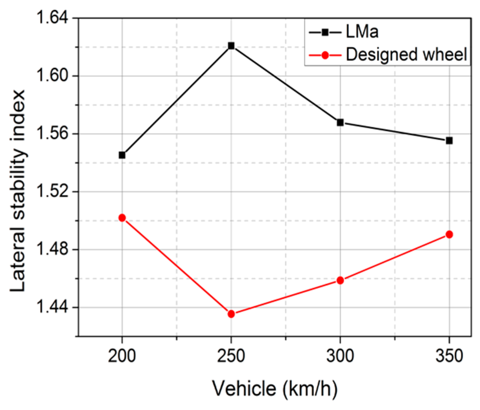
(2) Vehicle stability
The vehicle running stability is evaluated according to the Sperling stability indexes. In this paper, the vehicle speeds are set at 200, 250, 300 and 350 km/h. The U.S. Grade 6 railways track irregularity is adopted.
Figure 23 shows the comparative analysis of the lateral stability results for two types of wheels based on the Sperling stability indexes. It can be seen that the lateral stability of the optimized wheel at the 4 speed levels is better than that of the LMa profile and the running stability is improved by about 7%.
(3) Curve negotiation capability
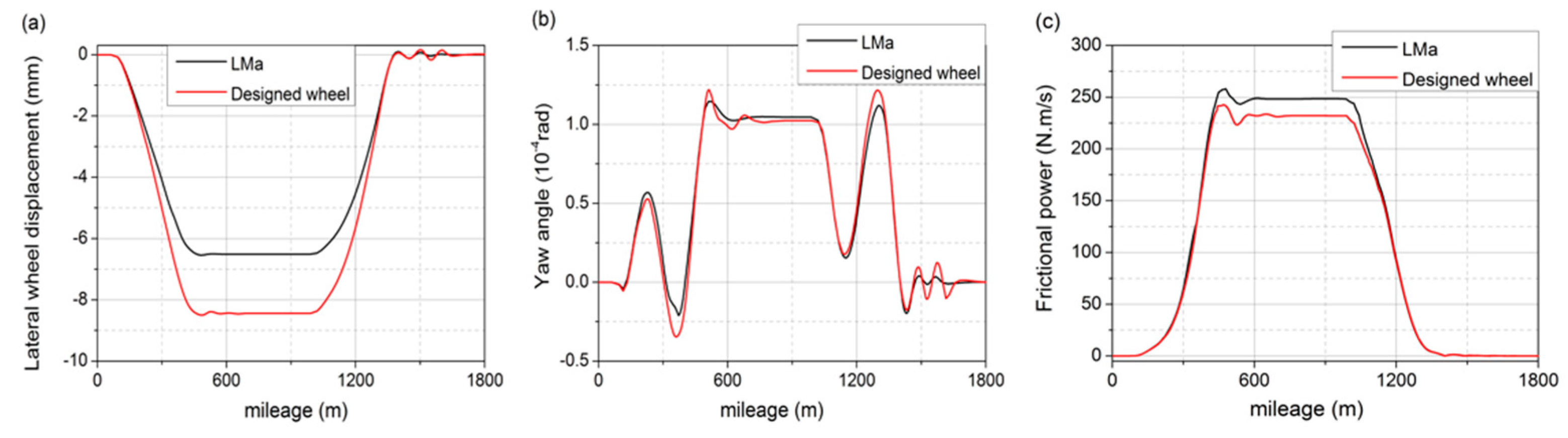
The speed of the vehicle passing the curve is set as 250 km/h. The parameters of the curve track are: circular curve length—500 m, radius length—3500 m, front/rear transition curve length—420 m, superelevation setting of outer rail—120 mm. The curve outlet and inlet are provided with 100 m straight lines. Figure 24 shows the simulated results. For the maximum dynamic response values, see Table 2.
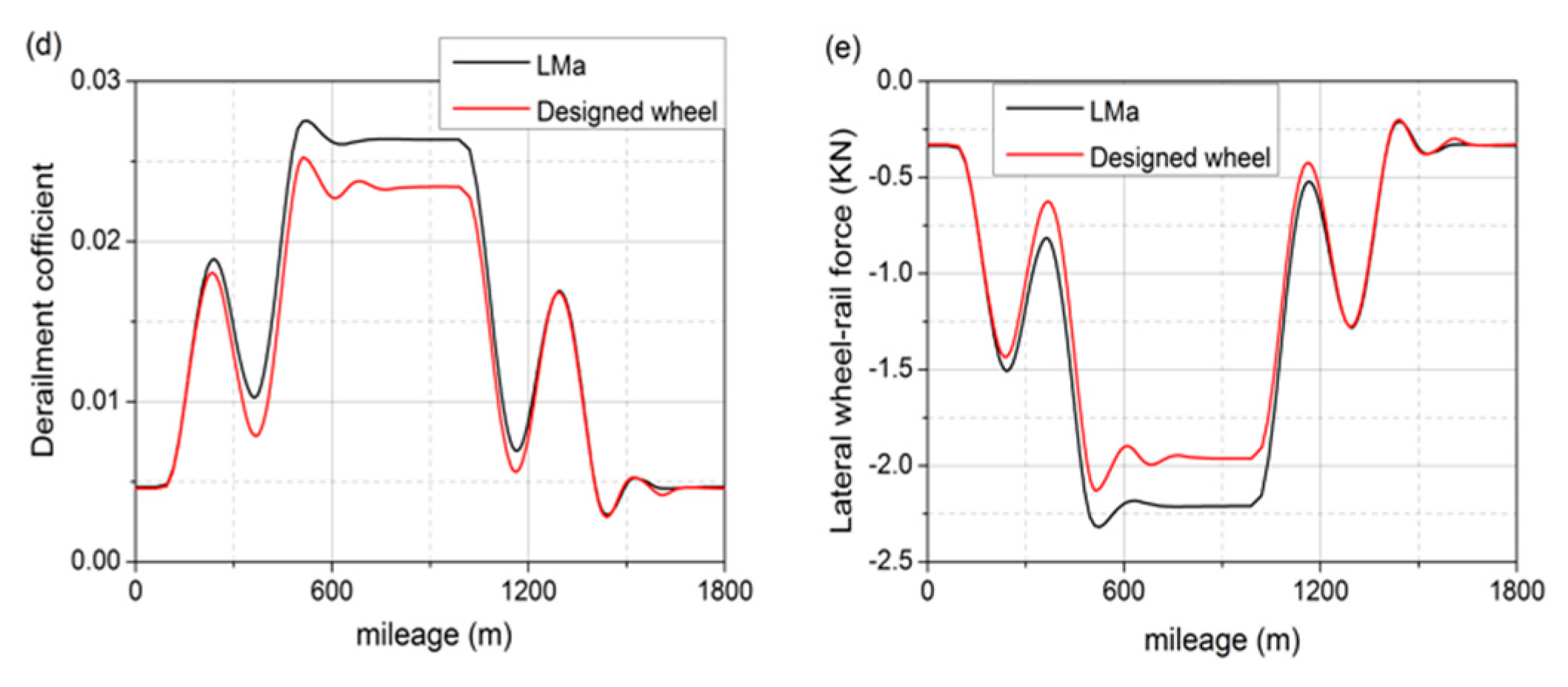
As shown in Figure 24 and Table 2, the lateral displacement of the first wheelset with optimized wheels on the curve line is greater than that of the LMa profile. When the optimized wheels match the CHN60 rail, the maximum lateral displacement of the front guide wheels of MU CRH2 is around 8.5 mm. The rolling angle of the first wheelset with optimized wheels is close to that of the LMa profile, the maximum yaw angle difference of the first wheelset is 0.08 rad. The outer wheel friction force, derailment coefficient and lateral wheel-rail force of the first wheelset with optimized wheels are better than those of the LMa profile. The results show that indexes regarding the curve negotiation capability of optimized wheels are better than those of LMa profiles when matching CHN60, except the lateral displacement of the first wheelset is slightly higher than that of LMa profiles.
6. Conclusions
This paper presents a reverse design method for wheel-rail profiles by taking the rolling radius difference as the target. This method consists of three parts, i.e., the profile designs of wheels, symmetric rails and non-symmetric rails. This method is deduced from the mapping relation between a rolling radius difference and a wheel-rail profile gradient. The designed wheel profile is a smooth curve created from a multi-sectional quadratic curve. Dichotomy is adopted during numerical calculation in order to improve the calculation efficiency.
The three reverse design examples (the profile designs of wheels, symmetric rails and non-symmetric rails) prove the effectiveness and efficiency of the method. This method is also suitable for optimization design of wheel profiles. The contrast analysis shows that when the lateral displacement reaches 6 mm, the maximum contact stress will be distributed evenly and can be decreased by 184.4 MPa compared to that of existing profiles. The critical speed can be increased by 10.8% compared to that of existing profiles. The running stability can be improved by around 7%.
This method is suitable for design of new-type wheel-rail profiles and optimization of existing profiles. This method, though having many advantages, still needs to be improved and optimized. The most important thing for this method is how to find the ideal rolling radius difference in order to design wheel-rail profiles satisfying the requirements and therefore more efforts are needed.
Acknowledgments
The present work has been supported by the National Natural Science Foundation of China (51425804, 51608459, 51778542, U1734207and 51378439).
Author Contributions
Jingmang Xu conceived the method; Rong Chen and Chenyang Hu built the mathematical model and analyzed the results; Rong Chen wrote the paper. Ping Wang supervised the entire work; Jiayin Chen and Yuan Gao wrote part of code.
Conflicts of Interest
The authors declare no conflict of interest.
References
- Souza, A.F.D. Influence of the wheel and rail treads profile on the hunting of the vehicles. Trans. ASME 1985, 107, 167–174. [Google Scholar]
- Enblom, R. Deterioration mechanisms in the wheel-rail interface with focus on wear prediction: A literature review. Veh. Syst. Dyn. 2009, 47, 661–700. [Google Scholar] [CrossRef]
- Magel, E.E.; Kalousek, J. The application of contact mechanics to rail profile design and rail grinding. Wear 2002, 253, 308–316. [Google Scholar] [CrossRef]
- An, B.; Wang, P.; Xu, J.; Chen, R.; Cui, D. Observation and Simulation of Axle Box Acceleration in the Presence of Rail Weld in High-Speed Railway. Appl. Sci. 2017, 7, 1259. [Google Scholar] [CrossRef]
- Heller, R.; Law, H.E. Optimizing the wheel profile to improve rail vehicle dynamic performance. Veh. Syst. Dyn. 1979, 8, 116–122. [Google Scholar] [CrossRef]
- Smith, R.; Kalouse, K.J. A design methodology for wheel and rail profiles for use on steered railway vehicles. Wear 1991, 144, 329–342. [Google Scholar] [CrossRef]
- Leary, J.F.; Handal, S.N. Development of freight car wheel profiles-a case study. Wear 1991, 144, 353–362. [Google Scholar] [CrossRef]
- Wu, H.M. Investigation of Wheel/Rail Interaction on Wheel Flange Climb Derailment and Wheel/Rail Profile Compatibility. Ph.D. Thesis, Illinois Institute of Technology, Chicago, IL, USA, 2000. [Google Scholar]
- Persson, I.; Iwnicki, S.D. Optimization of railway wheel profiles using a genetic algorithm. Veh. Syst. Dyn. 2004, 41, 517–527. [Google Scholar]
- Novales, M.; Orro, A.; Bugarin, M.R. Use of a genetic algorithm to optimize wheel profile geometry. Proc. Inst. Mech. Eng. Part F 2007, 221, 467–476. [Google Scholar] [CrossRef]
- Shevtsov, I.Y.; Markine, V.L.; Esveld, C. Optimal design of wheel profile for railway vehicles. Wear 2005, 258, 1022–1030. [Google Scholar] [CrossRef]
- Shevtsov, I.Y.; Markine, V.L.; Esveld, C. An inverse shape design method for railway wheel profiles. Struct. Multidiscip. Optim. 2007, 33, 243–253. [Google Scholar] [CrossRef]
- Shevtsov, I.Y.; Markine, V.L.; Esveld, C. Design of railway wheel profile taking into account of rolling contact fatigue and wear. Wear 2005, 265, 1273–1282. [Google Scholar] [CrossRef]
- Jahed, H.; Farshi, B.; Eshraghi, M.A.; Nasr, A. A numerical optimization technique for design of wheel profiles. Wear 2008, 264, 1–10. [Google Scholar] [CrossRef]
- Polach, O. Wheel profile design for target conicity and wide tread wear spreading. Wear 2011, 271, 195–202. [Google Scholar] [CrossRef]
- Gerlici, J.; Lack, T. Railway wheel and rail head profiles development based on the geometric characteristics shapes. Wear 2011, 271, 246–258. [Google Scholar] [CrossRef]
- Igensti, M.; Innocenti, A.; Marini, L.; Meli, E.; Rindi, A.; Toni, P. Wheel profile optimization on railway vehicles from the wear viewpoint. Int. J. Non-Linear Mech. 2103, 53, 41–54. [Google Scholar] [CrossRef]
- Igensti, M.; Marini, L.; Meli, E.; Rindi, A. Development of a Model for the Prediction of Wheel and Rail Wear in the Railway Field. J. Comput. Nonlinear Dyn. 2012, 7, 041004-1–041004-14. [Google Scholar] [CrossRef]
- Shen, G.; Ayasse, J.B.; Choller, H.; Pratt, I. A unique design method for wheel profiles by considering the contact angle function. Proc. Inst. Mech. Eng. Part F 2003, 217, 25–30. [Google Scholar] [CrossRef]
- Shen, G.; Zhong, X.B. A design method for wheel profiles according to the rolling radius difference function. Proc. Inst. Mech. Eng. Part F 2011, 225, 457–462. [Google Scholar] [CrossRef]
- Mao, X.; Shen, G. An inverse design method for rail grinding profiles. Veh. Syst. Dyn. 2017, 55, 1029–1044. [Google Scholar] [CrossRef]
- Mao, X.; Shen, G. A design method for rail profiles based on the geometric characteristics of wheel-rail contact. Proc. Inst. Mech. Eng. Part F 2017, 0, 1–11. [Google Scholar] [CrossRef]
- Xu, J.M.; Wang, P.; Wang, L.; Chen, R. Effects of profile wear on wheel-rail contact conditions and dynamic interaction of vehicle and turnout. Adv. Mech. Eng. 2016, 8, 1–14. [Google Scholar] [CrossRef]
Figure 1.
Wheel-rail contact.
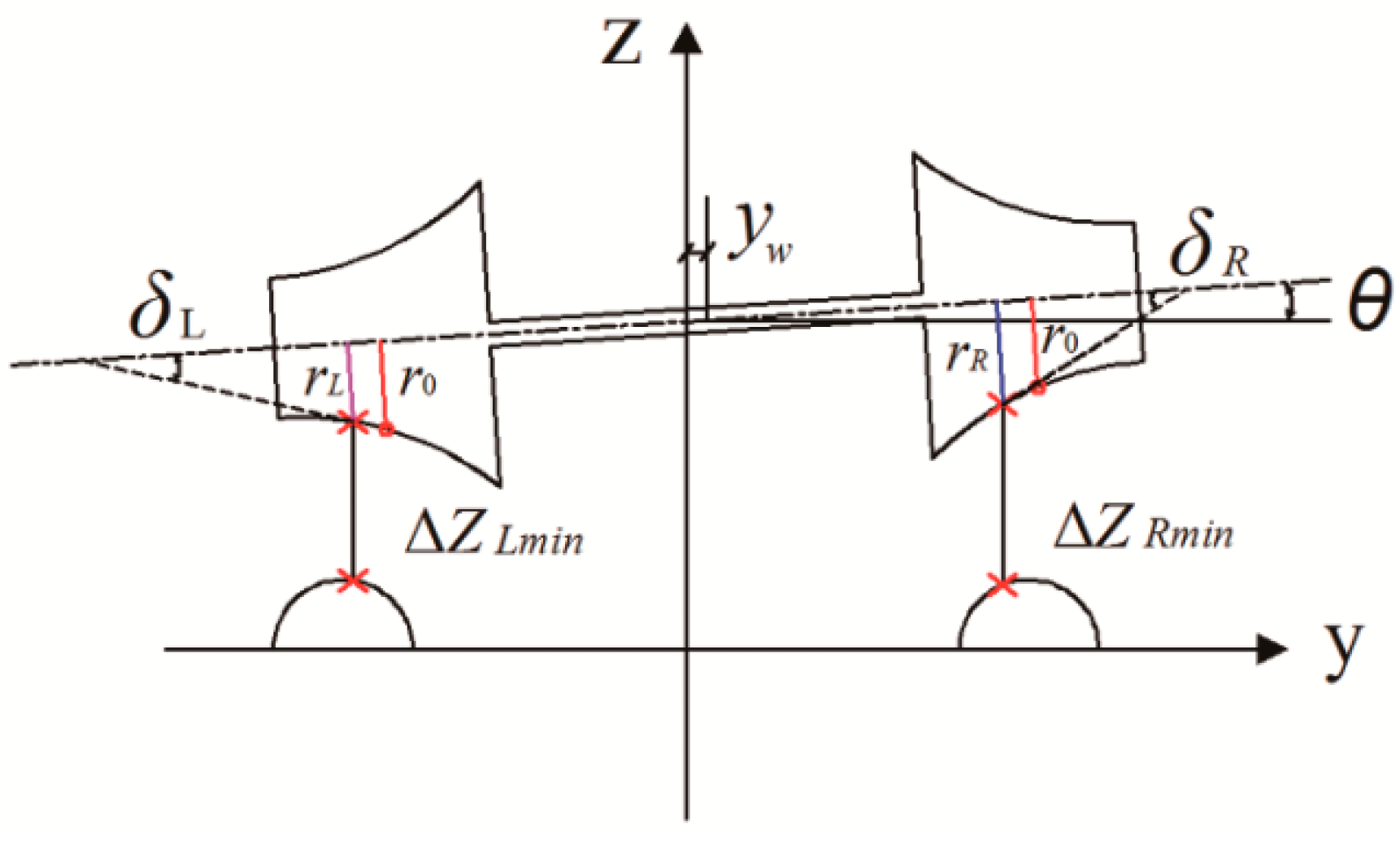
Figure 2.
Right wheel-rail contact demonstrated using the wheel-rail profile gradient.
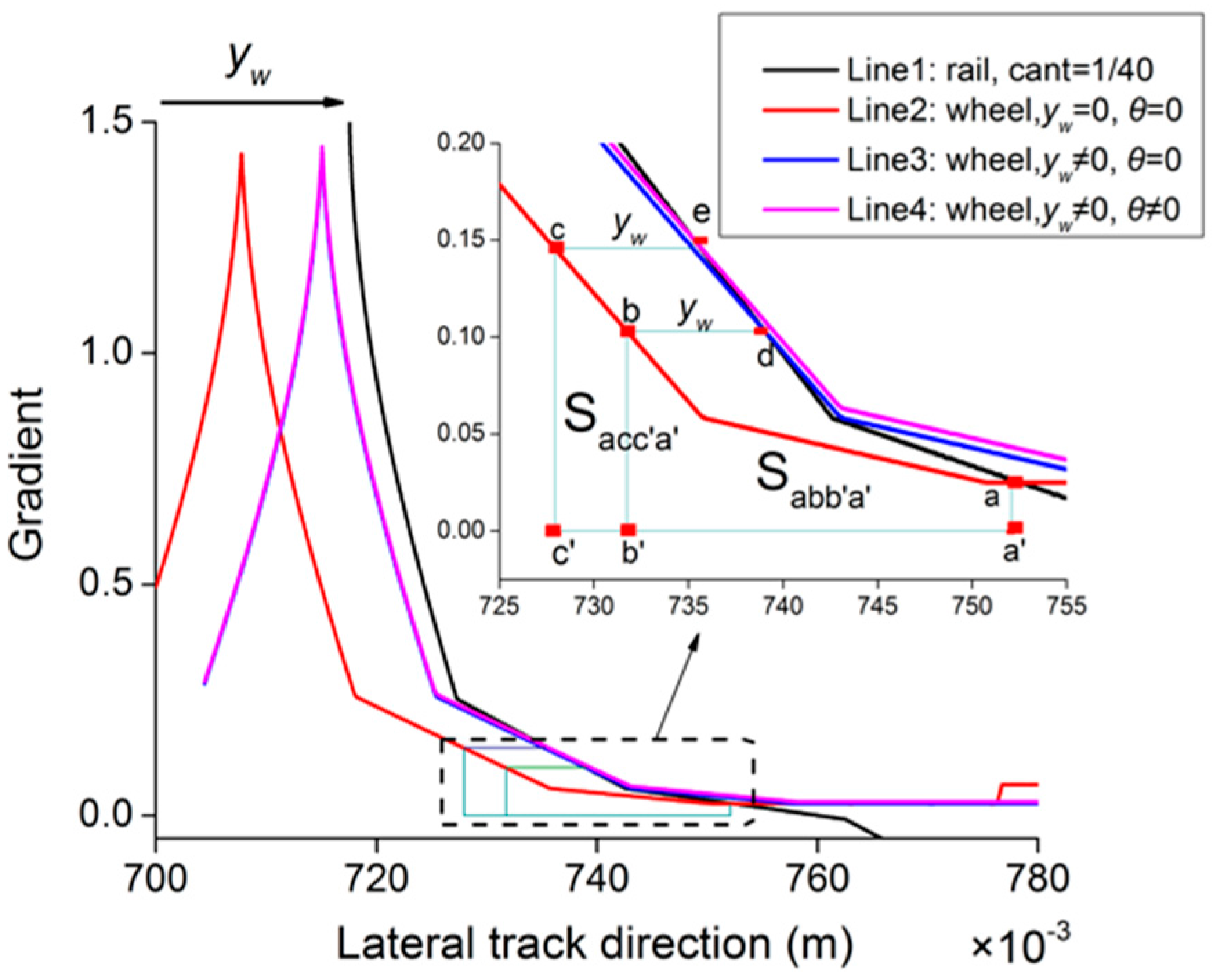
Figure 3.
Wheel-rail contact with different wheel profile gradients, without considering rolling angle. (a) Left wheel-rail; (b) Right wheel-rail.
Figure 3.
Wheel-rail contact with different wheel profile gradients, without considering rolling angle. (a) Left wheel-rail; (b) Right wheel-rail.

Figure 4.
Wheel-rail contact for wheel profile of Line 2.

Figure 5.
Reverse design of wheel profiles.
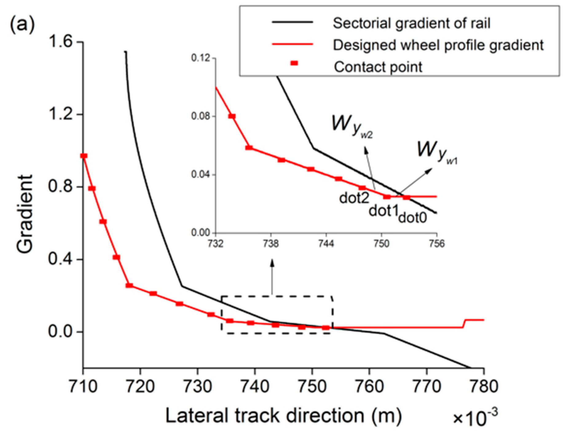
Figure 6.
Reverse design of wheel profile section .

Figure 7.
Flowchart.

Figure 8.
Reverse designed wheel profile and rolling radius difference. (a) Comparison between reverse designed profile and LMa profile; (b) Comparison between rolling radius differences.
Figure 8.
Reverse designed wheel profile and rolling radius difference. (a) Comparison between reverse designed profile and LMa profile; (b) Comparison between rolling radius differences.
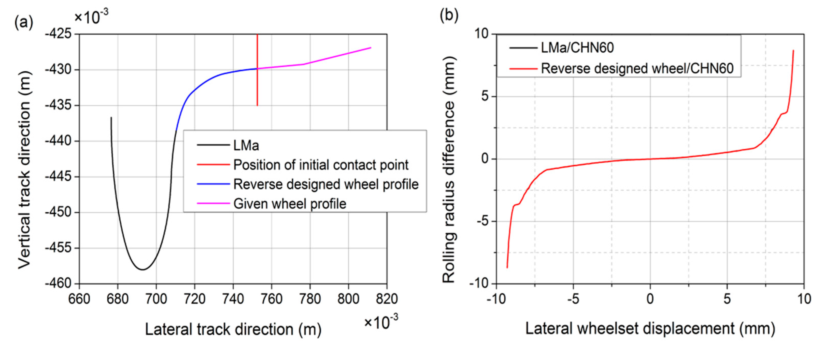
Figure 9.
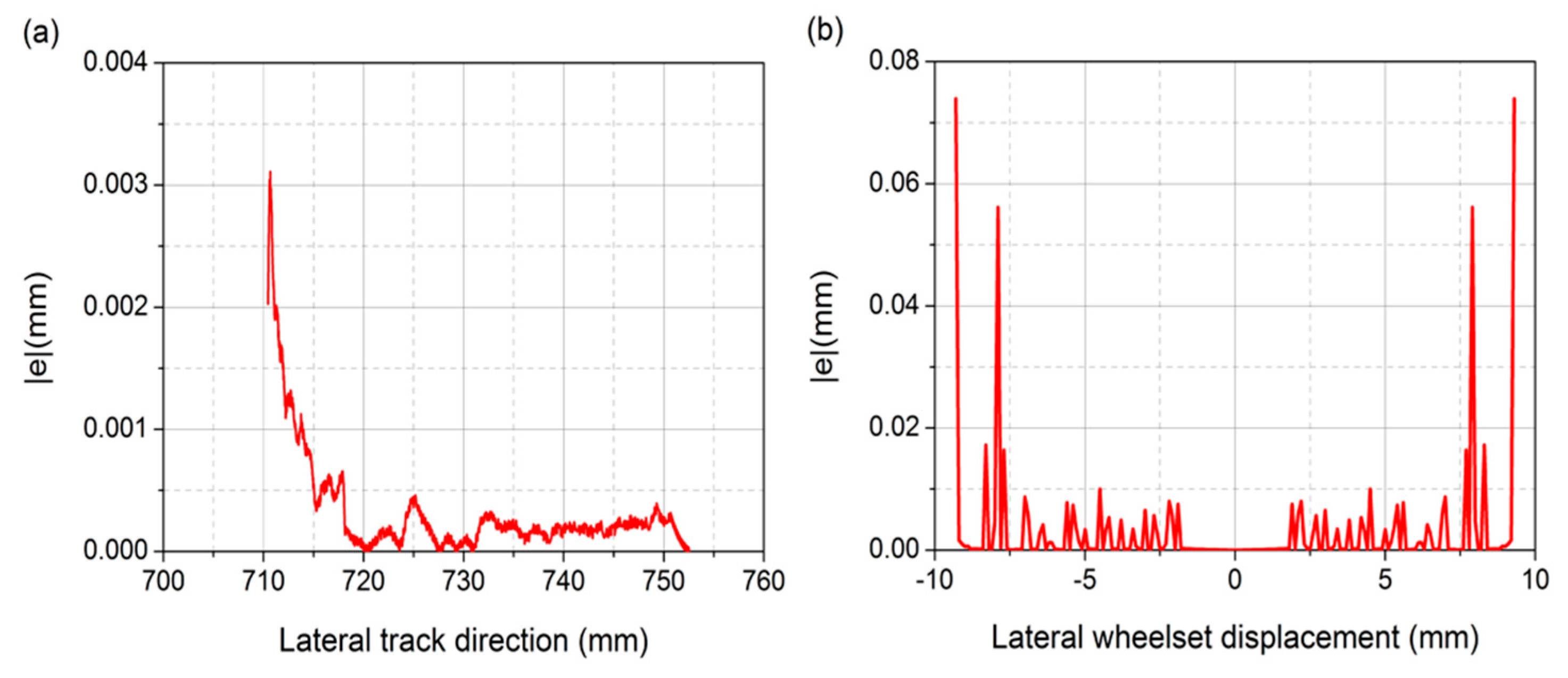
Absolute value of the error e. (a) wheel profile; (b) rolling radii difference distribution.
Figure 9.
Absolute value of the error e. (a) wheel profile; (b) rolling radii difference distribution.

Figure 10.
Reverse designed wheel profile and rolling radius difference. (a) Comparison between reverse designed profile and CHN60 profile; (b) Comparison between rolling radius differences.
Figure 10.
Reverse designed wheel profile and rolling radius difference. (a) Comparison between reverse designed profile and CHN60 profile; (b) Comparison between rolling radius differences.
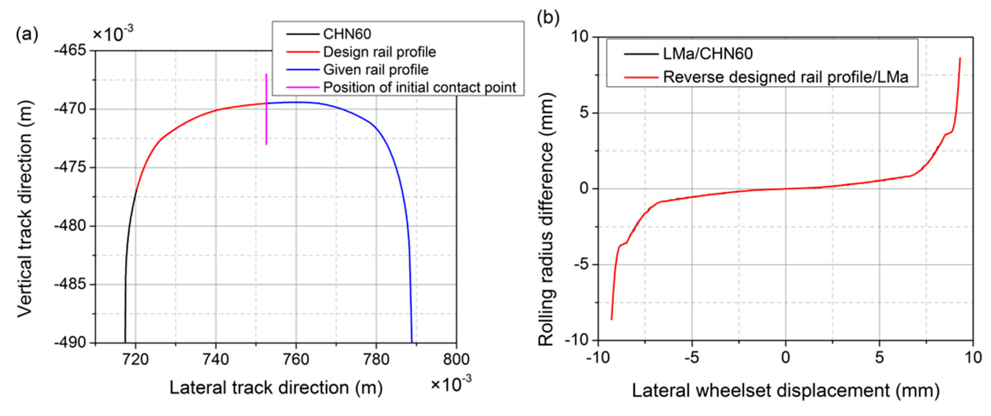
Figure 11.
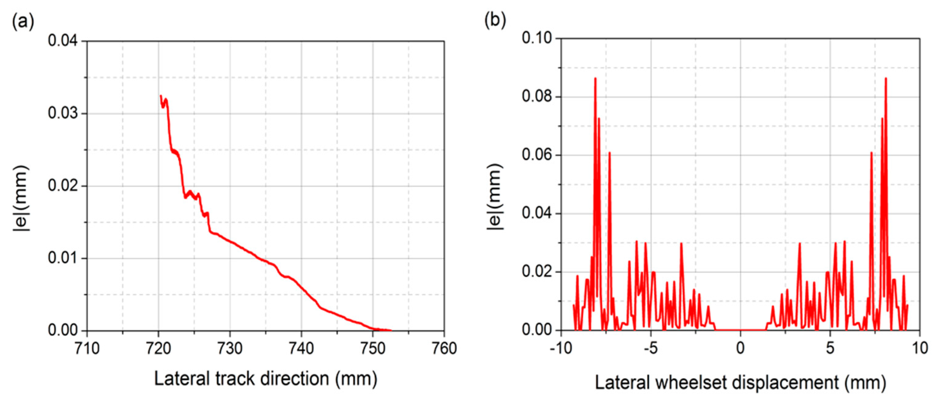
Absolute value of the error e. (a) rail profile; (b) rolling radii difference distribution.
Figure 11.
Absolute value of the error e. (a) rail profile; (b) rolling radii difference distribution.

Figure 12.
Reverse designed wheel profile and rolling radius difference. (a) Reverse designed wheel profile; (b) Comparison between rolling radius differences.
Figure 12.
Reverse designed wheel profile and rolling radius difference. (a) Reverse designed wheel profile; (b) Comparison between rolling radius differences.

Figure 13.
Absolute value of the error e in rolling radii difference distribution.

Figure 14.
Wheel-rail contact distribution at both sides. (a) Left LMa profile and CHN60; (b) Right LMa profile and reverse designed rail profile.
Figure 14.
Wheel-rail contact distribution at both sides. (a) Left LMa profile and CHN60; (b) Right LMa profile and reverse designed rail profile.
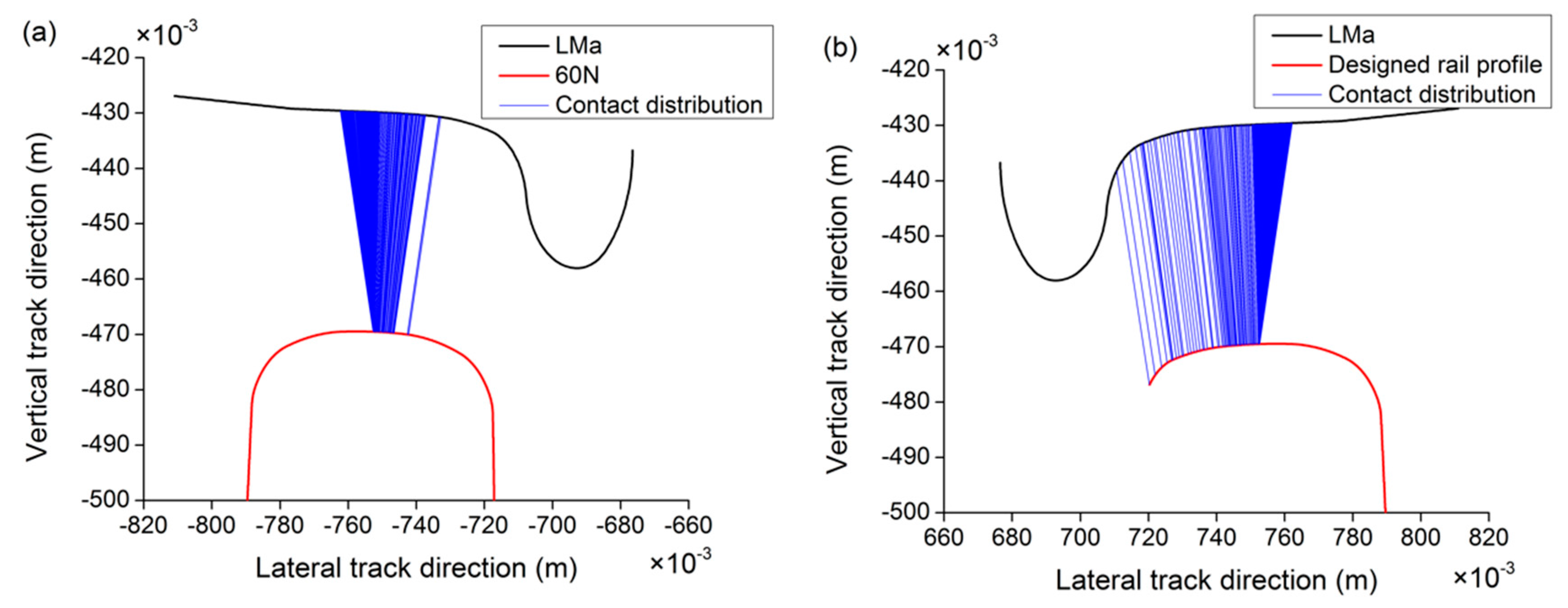
Figure 15.
Wheel profile and rolling radius difference. (a) Wheel profile; (b) Rolling radius difference.
Figure 15.
Wheel profile and rolling radius difference. (a) Wheel profile; (b) Rolling radius difference.
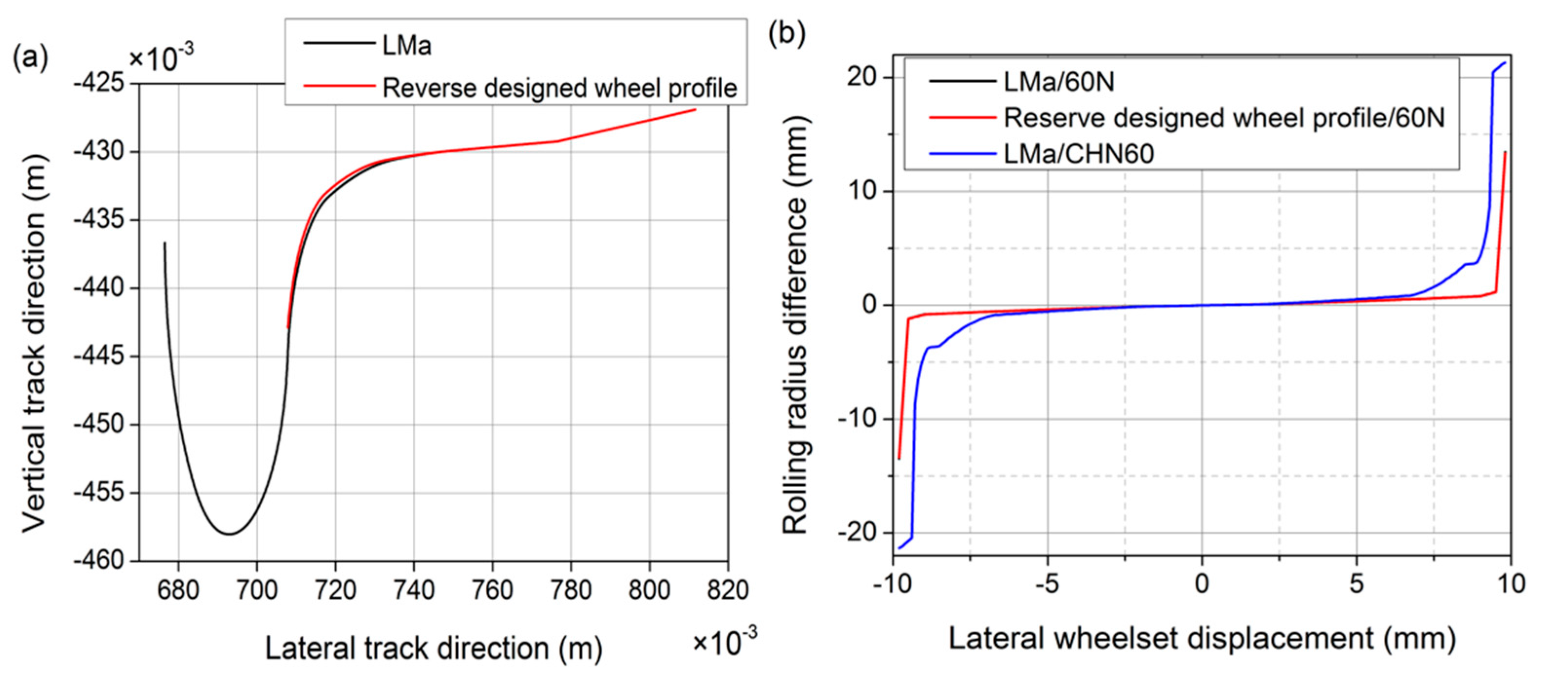
Figure 16.
Absolute value of the error e in rolling radii difference distribution.

Figure 17.
Wheel-rail contact distribution. (a) LMa and CHN60; (b) Optimized wheel and CHN60.

Figure 18.
Contact bandwidth and contact bandwidth ratio. (a) Contact bandwidth; (b) Contact bandwidth ratio.
Figure 18.
Contact bandwidth and contact bandwidth ratio. (a) Contact bandwidth; (b) Contact bandwidth ratio.
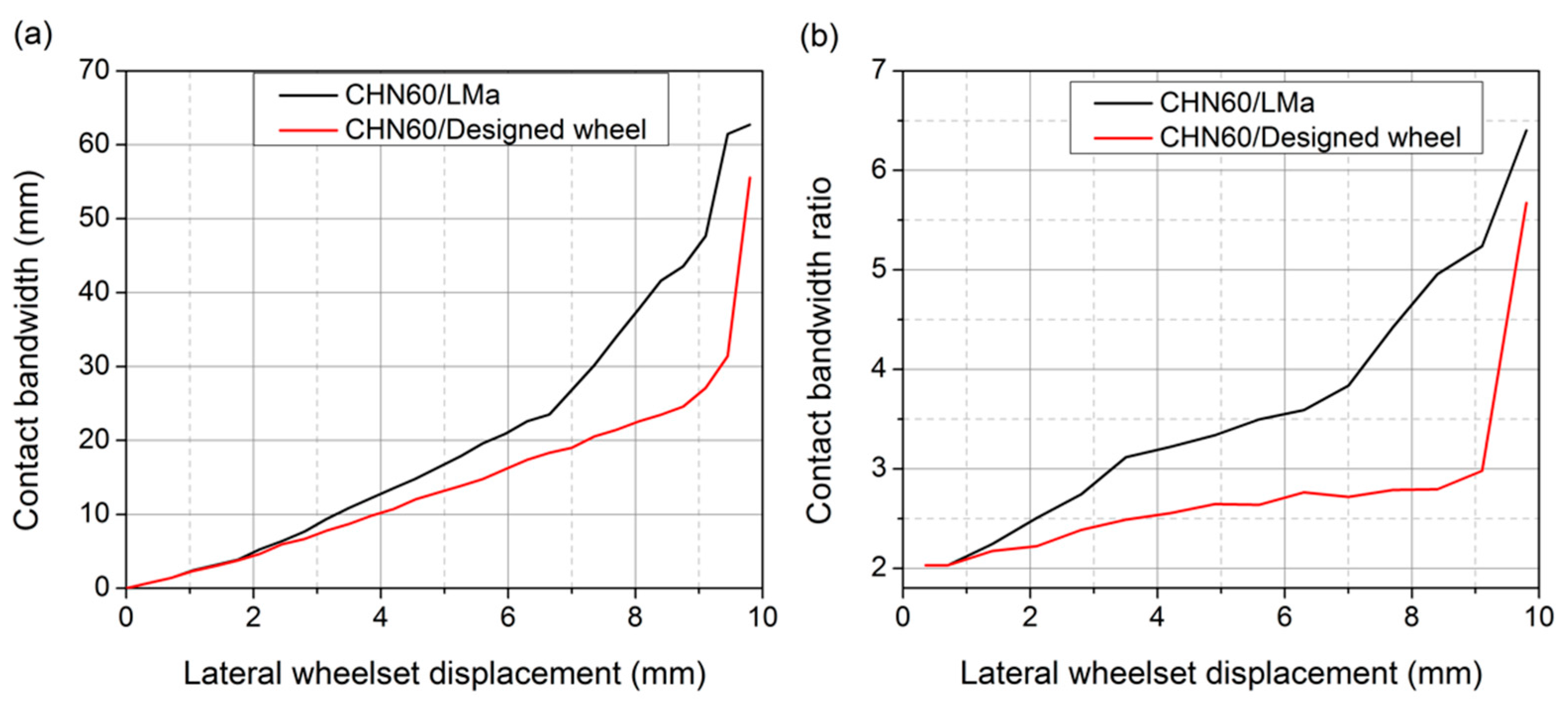
Figure 19.
LMa matching CHN60. (a) Lateral displacement 0 mm; (b) Lateral displacement 3 mm; (c) Lateral displacement 6 mm.
Figure 19.
LMa matching CHN60. (a) Lateral displacement 0 mm; (b) Lateral displacement 3 mm; (c) Lateral displacement 6 mm.

Figure 20.
Designed wheel matching CHN60. (a) Lateral displacement 0 mm; (b) Lateral displacement 3 mm; (c) Lateral displacement 6 mm.
Figure 20.
Designed wheel matching CHN60. (a) Lateral displacement 0 mm; (b) Lateral displacement 3 mm; (c) Lateral displacement 6 mm.

Figure 21.
Maximum wheel-rail contact stress at different lateral wheelset displacement.
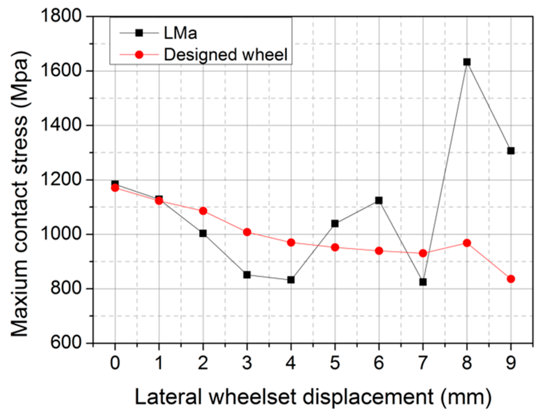
Figure 22.
Critical speed.

Figure 23.
Lateral stability index.

Figure 24.
Vehicle curve negotiation performance indexes. (a) Lateral displacement of the first wheelset; (b) Yaw angle of the first wheelset; (c) Wheel friction force of the first wheelset at the outer rail side; (d) Derailment coefficient of the first wheelset at the outer rail side; (e) Lateral wheel-rail force of the first wheelset at the outer rail side.


Table 1.
Maximum wheel-rail contact stress.
| Wheel Type | Max. Contact Stress (MPa) | ||
|---|---|---|---|
| Lateral Displacement 0 mm | Lateral Displacement 3 mm | Lateral Displacement 6 mm | |
| LMa | 1183.6 | 850.92 | 1123.6 |
| Optimized wheel | 1170.9 | 1008.4 | 939.2 |
Table 2.
Maximum dynamic parameters for vehicle curve negotiation.
| Dynamic Response | CHN60/LMa | CHN60/Optimized Wheel |
|---|---|---|
| Lateral wheel-rail force of the first wheelset at outer rail side (kN) | 2.3 | 2.1 |
| Friction power of the first wheelset at outer rail side (Nm/s) | 258 | 243 |
| Derailment coefficient of the first wheelset at outer rail side | 0.028 | 0.025 |
| Lateral displacement of the first wheelset (mm) | 6.5 | 8.5 |
| Attack angle of the first wheelset (rad) | 1.14 × 10⁻⁴ | 1.22 × 10⁻⁴ |
© 2018 by the authors. Licensee MDPI, Basel, Switzerland. This article is an open access article distributed under the terms and conditions of the Creative Commons Attribution (CC BY) license (http://creativecommons.org/licenses/by/4.0/).
Share and Cite
MDPI and ACS Style
Chen, R.; Hu, C.; Xu, J.; Wang, P.; Chen, J.; Gao, Y. An Innovative and Efficient Method for Reverse Design of Wheel-Rail Profiles. Appl. Sci. 2018, 8, 239. https://doi.org/10.3390/app8020239
AMA Style
Chen R, Hu C, Xu J, Wang P, Chen J, Gao Y. An Innovative and Efficient Method for Reverse Design of Wheel-Rail Profiles. Applied Sciences. 2018; 8(2):239. https://doi.org/10.3390/app8020239
Chicago/Turabian StyleChen, Rong, Chenyang Hu, Jingmang Xu, Ping Wang, Jiayin Chen, and Yuan Gao. 2018. "An Innovative and Efficient Method for Reverse Design of Wheel-Rail Profiles" Applied Sciences 8, no. 2: 239. https://doi.org/10.3390/app8020239
Note that from the first issue of 2016, this journal uses article numbers instead of page numbers. See further details here.