Trajectory Tracking of an Omni-Directional Wheeled Mobile Robot Using a Model Predictive Control Strategy

Abstract

This paper addresses trajectory tracking of an omni-directional mobile robot (OMR) with three mecanum wheels and a fully symmetrical configuration. The omni-directional wheeled robot outperforms the non-holonomic wheeled robot due to its ability to rotate and translate independently and simultaneously. A kinematics model of the OMR is established and a model predictive control (MPC) algorithm with control and system constraints is designed to achieve point stabilization and trajectory tracking. Simulation results validate the accuracy of the established kinematics model and the effectiveness of the proposed MPC controller.

1. Introduction

Industrial automation is a prerequisite for intelligent manufacturing, and mobile robots represent a core component of industrial automation systems. In recent decades, due to the broad applications for mobile robots, the core issues in motion control of mobile robots, including point stabilization, path planning, trajectory tracking, and real-time avoidance, have attracted considerable attention from both academic scholars and practitioners [1,2,3,4,5].

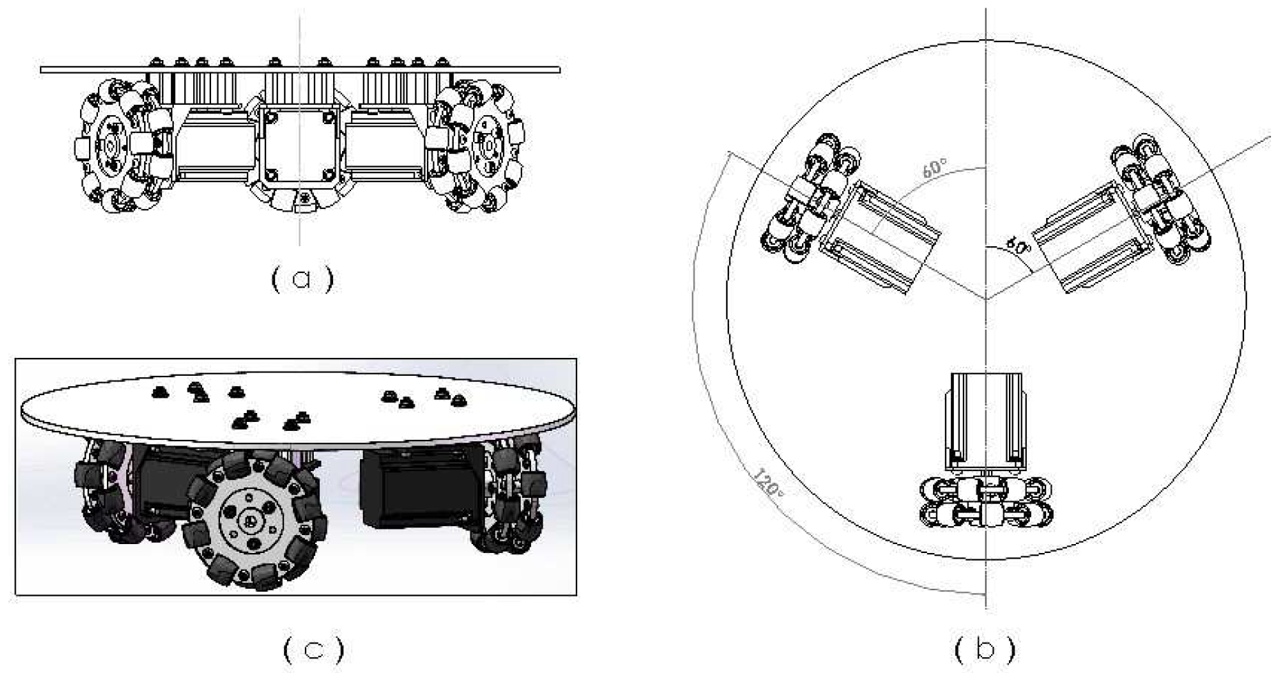
Although large numbers of mobile robots have begun to enter homes, hospitals, and many other industrial areas, mobile robots with new structures (as opposed to the traditional dual-drive wheeled mobile robots), are required to meet continuously increasing demands with respect to high flexibility, efficiency, and safety of complex and diverse applications in reality. Omni-directional mobile robots (OMRs) with mecanum wheels provide an alternative and have drawn much attention from researchers. In [6,7], two different omni-directional mobile structures with mecanum wheels were proposed. In [7,8], the kinematics of OMRs were analyzed and the motion control of robots was achieved. In [9], a comprehensive omni-directional soccer player robot with no head direction was proposed and it was capable of more sophisticated behaviors, such as ball passing and goal keeping. Compared with the traditional nonholonomic dual-drive wheeled robot, the omni-directional mobile robot is able to synchronize steering and linear motion in any direction. This advantage not only improves the flexibility of the robot greatly in order to achieve fast target tracking and obstacle avoidance, but also provides more references for robot motion control methods.

Motion control is a core issue in the mobile robot system and guarantees the smooth movement of the robot. Due to the diversity of motion and increasing performance requirements, motion control algorithms are becoming more and more complex. In [10], a receding horizon (RH) controller was developed for the tracking control of a nonholonomic mobile robot. In [11], a novel biologically inspired tracking control approach for real-time navigation of a nonholonomic mobile robot was proposed by integrating a backstepping technique and a neurodynamics model. In [12], an approach was proposed for complete characterization of the shortest paths to a goal position and it was used for path planning of the robot. A novel method referred to as the visibility binary tree algorithm for robot navigation with global information was introduced in [13]. The set of all complete paths between the robot and target in the global environment with some circle obstacles was obtained by using the tangent visibility graph. Then, an algorithm based on the visibility binary tree created for the shortest paths was run to obtain the optimal path for the robot. In [14], a real-time obstacle avoidance approach for mobile robots was presented based on the artificial potential field concept. The motion control of omni-directional mobile robot has also been investigated and many results have been reported [15,16,17,18]. Among them, the model predictive control (MPC) algorithm is the most common control method used for trajectory tracking of the OMR.

The MPC algorithm is an efficient predictive control technique and is composed of model prediction, rolling optimization, and feedback correction. The MPC algorithm has been widely used in industrial control applications and is able to take various constraints into consideration. The core of MPC control problem finding the optimal solution of a cost function constructed according to the error between system output at the sampling time and the predicted output of the established prediction system model. The optimal solution is taken as the optimal control input in the future prediction time domain and the first control vector of the optimal solution is used as the real control input. The advantages of the MPC algorithm are: (1) It is easy to model; (2) It has a rolling optimization strategy with good dynamic control effect; (3) It can correct the output by feedback which improves the robustness of the control system; (4) As a computer optimization control algorithm, it is easy to realize on a computer. In recent years, the MPC algorithm has also been widely used to achieve optimized motion control of mobile robots. In [19], a novel visual servo-based model predictive control method was proposed to steer a wheeled mobile robot moving in a polar coordinate. In [20], a model-predictive trajectory-tracking controller, which used linearized tracking-error dynamics to predict future system behavior, was presented. In [21], a state feedback MPC method was proposed and applied for trajectory tracking of a three-wheeled OMR. The cost function in the proposed MPC method is constructed over finite horizon and is optimized in the linear matrix inequalities (LMI) framework. In [22], a virtual-vehicle concept and an MPC strategy were combined to handle robot motion constraints and the path-following problem.

In this paper, the kinematic analysis of the OMR is conducted and then an MPC algorithm for point stabilization and trajectory tracking is proposed. In the proposed MPC controller, the rotation speeds of the three wheels and the state outputs of the robot are taken as manipulated variables and controlled variables, respectively. In stabilization control of the robot, a target point and an arbitrary initial direction, which lie within a given constraint range of the coordinate, are set and then the robot tracks the target point and stabilizes itself automatically. In the trajectory tracking of the robot, a pulsed route is planned and different target angles at each node point are set. The robot can move from the start point of the trajectory to the end point along the given route with target angles.

This paper is organized as follows: A brief description and kinematics analysis of the considered OMR are given in Section 2. Section 3 presents the MPC strategy including MPC elements and the optimization method. Simulation results of the proposed MPC algorithm are presented in Section 4. Finally, Section 5 concludes the work in this paper.

2. Omni-Directional Wheeled Mobile Robot Model

2.1. Omni-Directional Mobile Structure

The concept of the mecanum wheel was proposed by a Swedish mecanum company. The mecanum wheel is mainly composed of a motor-controlled wheel hub and some passive rollers, which are evenly distributed at a certain angle along the outer edge of the wheel.

The mecanum wheels used in this paper are light-load ${90}^{°}$ omni-directional CL-10 wheels produced by Chengdu Hangfa Hydraulic Engineering Co., Ltd. (Chengdu, China). As shown in Figure 1, the outer diameter of the mecanum wheel is 101.6 mm and it has 16 rollers distributed in both of outer sides. The rollers can rotate in a perpendicular direction to the hub rotation and the envelopes on the outside of these rollers form a cylindrical surface, which enables smooth movement of the wheel. Each roller is equipped with two nylon sliding bearings, which gives the wheels good wear resistance and flexibility. Each wheel can withstand loads of up to 50 kg. Therefore, this series of mecanum wheels is a good choice for lightly-loaded omni-directional wheeled mobile platforms.

As shown in the bottom view of the OMR in Figure 2b, the platform is equipped with three motors and each motor is used to control one mecanum wheel. The axes of these three motors join at the center of the chassis and the angles between the neighboring two motors are the same. In Figure 2a,c, the front view and the overall model of the platform diagram are shown, respectively. Based on the characteristics of mecanum wheel and the analysis of system model, the platform can conduct omnidirectional motion with the advantages of strong adaptability, high sensitivity, good stability, and flexible rotation.

2.2. Kinematics Model

For the OMR, each wheel has two position parameters: the position relative to the center of the platform, and the respective attitude angle. The coordinates of the mecanum wheel are shown in Figure 3. In this figure, $xoy$ is the coordinate frame attached to the center of the platform, $x^{\prime }{o}^{\prime }{y}^{\prime }$ is a coordinate frame attached to the axis center of one mecanum wheel, i represents the order of the mecanum wheel, ${\alpha }_i$ is the deflection angle of each roller, ${\beta }_i$ is the angle between lines $\overline{o{o}^{\prime }}$, and $\overline{ox}$, $\left(l_{ix},l_{iy},{\theta }_i\right)$ are the wheel’s location and pose, respectively, in the coordinate $xoy$. $l_{ix}$ and $l_{iy}$ can be expressed as

$$l_{ix}=l_i\cos {\beta }_i,l_{iy}=l_i\sin {\beta }_i$$

(1)

The structure of mecanum wheel is shown in Figure 4. In this figure, r denotes radius of the mecanum wheel, $V_{ir}$ denotes velocity vector of the roller center, and ${\omega }_i$ denotes rotation velocity of the motor. There are three speed vectors. ${\left[v_x{v}_y\omega \right]}^T$ describes the center speed of the platform relative to the ground, ${\left[v_{ix}{v}_{iy}{\omega }_i\right]}^T$ presents the center speed of the mecanums wheels relative to the coordinate $xoy$, and ${\left[{v^{\prime }}_{ix}{v^{\prime }}_{iy}{{\omega }^{\prime }}_i\right]}^T$ denotes the center speed of the mecanums relative to the coordinate $x^{\prime }{o}^{\prime }{y}^{\prime }$. The kinematic models of the OMR are described as

$$\left[\begin{array}{c}{v^{\prime }}_{ix}\\ {v^{\prime }}_{iy}\end{array}\right]=K_{i1}\left[\begin{array}{c}{\omega }_i\\ v_{ir}\end{array}\right],K_{i1}=\left[\begin{array}{cc}0& \sin {\alpha }_i\\ r& \cos {\alpha }_i\end{array}\right]$$

(2)

$$\begin{array}{c}\hfill \left[\begin{array}{c}{v}_{ix}\\ v_{iy}\end{array}\right]=K_{i2}\left[\begin{array}{c}{v^{\prime }}_{ix}\\ {v^{\prime }}_{iy}\end{array}\right]=K_{i2}{K}_{i1}\left[\begin{array}{c}{\omega }_i\\ v_{ir}\end{array}\right]K_{i2}=\left[\begin{array}{cc}\cos {\theta }_i& -\sin {\theta }_i\\ \sin {\theta }_i& \cos {\theta }_i\end{array}\right]\end{array}$$

(3)

$$\left[\begin{array}{c}{v}_{ix}\\ v_{iy}\end{array}\right]=K_{i3}\left[\begin{array}{c}{v}_x\\ v_x\\ \omega \end{array}\right],K_{i3}=\left[\begin{array}{ccc}1& 0& -l_{iy}\\ 0& 1& l_{ix}\end{array}\right]$$

(4)

Based on Equations (3) and (4) , the inverse kinematics equation of the system can be obtained as

$$K_{i2}{K}_{i1}\left[\begin{array}{c}{\omega }_i\\ v_{ir}\end{array}\right]=K_{i3}\left[\begin{array}{c}{v}_x\\ v_x\\ \omega \end{array}\right],i=1,2,3,$$

(5)

and $\det \left(K_{i2}{K}_{i1}\right)\ne 0$.

Assuming that

$$K_i={\left[K_{i1}\right]}^{-1}{\left[K_{i2}\right]}^{-1}\ast K_{i3},i=1,2,3,{\gamma }_i={\theta }_i-{\alpha }_i$$

then, the inverse kinematics equation of each mecanum wheel is derived as

$$\left[\begin{array}{c}{\omega }_i\\ v_{ir}\end{array}\right]={\left[K_{i1}\right]}^{-1}{\left[K_{i2}\right]}^{-1}{K}_{i3}\left[\begin{array}{c}{v}_x\\ v_y\\ \omega \end{array}\right]=K_i\left[\begin{array}{c}{v}_x\\ v_y\\ \omega \end{array}\right]$$

(6)

where

$$K_i=\frac{1}{-r\sin {\alpha }_i}\left[\begin{array}{ccc}\cos \left({\gamma }_i\right)& \sin \left({\gamma }_i\right)& l_{ix}\sin \left({\gamma }_i\right)-l_{iy}\cos \left({\gamma }_i\right)\\ r\cos {\theta }_i& -r\sin {\theta }_i& l_{iy}r\cos {\theta }_i-l_{ix}r\sin {\theta }_i\end{array}\right]$$

Assuming that

$$\mathrm{E}=\left[\begin{array}{ccc}\begin{array}{c}\frac{\cos \left({\gamma }_1\right)}{\sin {\alpha }_1}\\ \frac{\cos \left({\gamma }_2\right)}{\sin {\alpha }_2}\\ \frac{\cos \left({\gamma }_3\right)}{\sin {\alpha }_3}\end{array}& \begin{array}{c}\frac{\sin \left({\gamma }_1\right)}{\sin {\alpha }_1}\\ \frac{\sin \left({\gamma }_2\right)}{\sin {\alpha }_2}\\ \frac{\sin \left({\gamma }_3\right)}{\sin {\alpha }_3}\end{array}& \begin{array}{c}\frac{l_1\sin \left({\gamma }_1-{\beta }_1\right)}{\sin {\alpha }_1}\\ \frac{l_2\sin \left({\gamma }_2-{\beta }_2\right)}{\sin {\alpha }_2}\\ \frac{l_3\sin \left({\gamma }_3-{\beta }_3\right)}{\sin {\alpha }_3}\end{array}\end{array}\right]$$

the rotating speed of mecanum wheels is expressed as

$$\left[\begin{array}{c}{\omega }_1\\ {\omega }_2\\ {\omega }_3\end{array}\right]=\frac{1}{-r}E\left[\begin{array}{c}{v}_x\\ v_y\\ \omega \end{array}\right]$$

(7)

Based on the relationship $v=r\omega$, Equation (7) can be transformed into

$$v=\left[\begin{array}{c}{v}_1\\ v_2\\ v_3\end{array}\right]=-E\left[\begin{array}{c}\dot{x}\\ \dot{y}\\ \omega \end{array}\right]$$

(8)

Actually, the Cartesian motion control problems are the main issues in the research on mobile robots. The state of the OMR in Cartesian coordinate $x_c{o}_c{y}_c$ is denoted as $\left(x_c,y_c,{\theta }_c\right)$ and is shown in Figure 5.

According to Figure 5, it is derived that

$$\left[\begin{array}{c}{\dot{x}}_c\\ {\dot{y}}_c\\ {\omega }_c\end{array}\right]=\left[\begin{array}{ccc}\cos {\theta }_c& -\sin {\theta }_c& 0\\ \sin {\theta }_c& \cos {\theta }_c& 0\\ 0& 0& 1\end{array}\right]\left[\begin{array}{c}\dot{x}\\ \dot{y}\\ \omega \end{array}\right]$$

(9)

Assuming that

$$H=\left[\begin{array}{ccc}\cos {\theta }_c& -\sin {\theta }_c& 0\\ \sin {\theta }_c& \cos {\theta }_c& 0\\ 0& 0& 1\end{array}\right],$$

the inverse kinematics equation of the OMR in Cartesian coordinate can be transformed into

$$\left[\begin{array}{c}{v}_1\\ v_2\\ v_3\end{array}\right]=-E{H}^{-1}\left[\begin{array}{c}{\dot{x}}_c\\ {\dot{y}}_c\\ {\omega }_c\end{array}\right].$$

(10)

The Jacobian matrix of the inverse kinematics equation of the OMR is

$$\begin{array}{c}\hfill R=-E{H}^{-1}\end{array}$$

(11)

Actually, the Jacobi matrix of the inverse kinematics equation determines the OMR’s omni-directionality. If the Jacobi matrix is in the state of dissatisfied rank, there are some nonholonomic constraints in the structure and the degree of freedom movement is reduced, which means that the system cannot achieve all-round movement [23]. It can be derived that the necessary condition to achieve the all-round movement of OMR is $rank\left(R\right)=3$.

Through tests, the parameters of the OMR are obtained. They are shown in Figure 6 and

Table 1. The parameters of system structure.

Para	${\beta }_1$	${\beta }_2$	${\beta }_3$	${\theta }_1$	${\theta }_2$	${\theta }_3$	${\alpha }_1$	${\alpha }_2$	${\alpha }_3$
Value	${60}^{°}$	${180}^{°}$	${300}^{°}$	${60}^{°}$	${180}^{°}$	${300}^{°}$	${90}^{°}$	${90}^{°}$	${90}^{°}$

.

Substituting these parameters into Equation (10) yields

$$\left[\begin{array}{c}{v}_1\\ v_2\\ v_3\end{array}\right]=\left[\begin{array}{ccc}-0.866\cos {\theta }_c-0.5\sin {\theta }_c& 0.5\cos {\theta }_c-0.866\sin {\theta }_c& 0.16352\\ \sin {\theta }_c& -\mathrm{con}{\theta }_c& 0.16352\\ 0.866\cos {\theta }_c-0.5\sin {\theta }_c& 0.5\cos {\theta }_c+0.866\sin {\theta }_c& 0.16352\end{array}\right]\left[\begin{array}{c}{\dot{x}}_c\\ {\dot{y}}_c\\ {\omega }_c\end{array}\right]$$

(12)

It can be derived from the result that $rank\left(R\right)=3$, which means the OMR can achieve all-round movement.

3. MPC Strategy

The MPC algorithm has been widely used in motion control of mobile robots and it has three basic characteristics: model prediction, rolling optimization, and feedback correction. It has unique advantages for solving motion control problems, such as point stabilization and trajectory tracking of mobile robots. Traditional methods often neglect or simplify the robot kinematics and dynamics constraints which have a significant impact on the robot’s control performance. Meanwhile, the MPC algorithm takes the constraints into consideration to improve the system robustness. The existing controllers have high requirements with respect to the accuracy of the system model and tend to obtain effective control parameters based on the model and multiple experimental tests;. However, the MPC algorithm has low requirements with respect to the accuracy of the system model and can acquire the control parameters through simple experiments. Through applying the characteristics of rolling optimization and feedback correction, the influence of time-delay in the closed-loop system can be effectively reduced or even eliminated, and the motion control is optimized to achieve improved control performance. Particularly, the MPC algorithm can handle multivariate and constrained problems effectively.

The MPC problem can be described as solving the optimal solution of the cost function. At each sampling time, the outputs of the future N sampling instants are predicted according to the system model, and the cost function is constructed based on the errors between the predicted outputs and the true state outputs of the system. The optimal control inputs of the next N sampling instants are obtained by minimizing the cost function, however, only the first control vector is used as the system input. At the next sampling time, this process is repeated and rolling optimization is performed.

In this section, an MPC-based kinematic controller is designed to ensure that the mobile robot can be driven to the desired position accurately, smoothly, and stably.

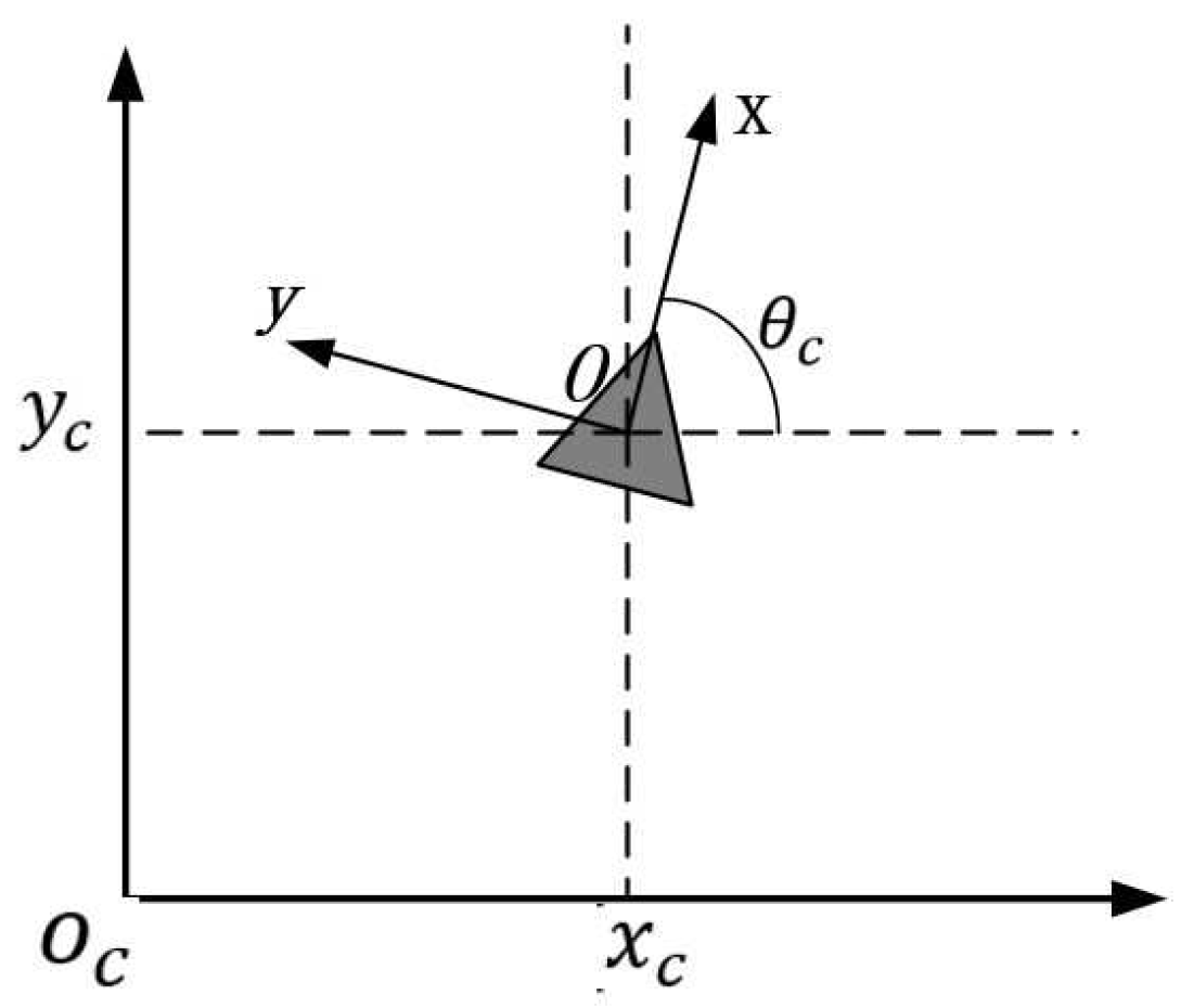
Define $q={\left[x_c{y}_c{\theta }_c\right]}^T$ as the state of mobile robot in coordinate $x_c{o}_c{y}_c$ and $S={\left[S_1{S}_2{S}_3\right]}^T=R^{-1}$. Then, it can be derived that

$$\dot{q}\left(t\right)=S\left(t\right)v\left(t\right)$$

(13)

where

$$\begin{array}{cc}\hfill S_1\left(t\right)& ={\left[\begin{array}{c}-0.5774\cos {\theta }_c\left(t\right)-0.3333\sin {\theta }_c\left(t\right)\\ 0.6667\sin {\theta }_c\left(t\right)\\ 0.5774\cos {\theta }_c\left(t\right)-0.3333\sin {\theta }_c\left(t\right)\end{array}\right]}^T\hfill \\ \hfill S_2\left(t\right)& ={\left[\begin{array}{c}0.3333\cos {\theta }_c\left(t\right)-0.5774\sin {\theta }_c\left(t\right)\\ -0.6667\cos {\theta }_c\left(t\right)\\ 0.3333\cos {\theta }_c\left(t\right)+0.5774\sin {\theta }_c\left(t\right)\end{array}\right]}^T\hfill \\ \hfill S_3\left(t\right)& =\left[\begin{array}{ccc}0.002038& 0.002038& 0.002038\end{array}\right]\hfill \end{array}$$

Based on zero-order hold (ZOH), a continuous-time system can be transformed into a discrete-time form with a sampling period T.

$$q\left(k+1\right)=q\left(k\right)+\dot{q}\left(k\right)T$$

(14)

The discrete-time system (14) can be transformed into a discrete state space system as

$$q(k+1)=Aq\left(k\right)+Bu\left(k\right)$$

(15)

where

$$A=I\in {\mathbb{R}}^{n\times n},B=S\left(k\right)T\in {\mathbb{R}}^{n\times m}$$

The parameter n is the number of state variables and m is the number of input variables. The matrix A is a constant identity matrix, and matrix B is determined by orientation of the system dynamically.

Based on the state space model (15), the MPC algorithm is designed to control the system. Here, a cost function is required and optimized through solving a quadratic program (QP) problem to obtain the optimal control sequence in predictive horizon N. The cost function for the MPC can be defined as

$$J\left(k\right)=\sum _{j=1}^N\left[{∥q(k+j|k)∥}_Q^2+{∥u(k+j-1|k)∥}_R^2\right]$$

(16)

where $Q\in {\mathbb{R}}^{n\times n}$ and $R\in {\mathbb{R}}^{m\times m}$ are appropriate weighting matrices. $q(k+j|k)$ and $u(k+j-1|k)$ denote the predicted state and control vector in predictive horizon at time k.

Through solving the following finite-horizon optimal control problem online, the optimal control sequence can be obtained.

$$u^{*}=\arg \underset{u}{\min }\left\{J\left(k\right)\right\}$$

(17)

Since the torques generated by motors are limited by the performance of the motors, the $u\left(k\right)$ has an upper and lower bound, and the range of state variable $q\left(k\right)$ is also constrained. Thus, the following constraints should be imposed on the system:

$$\begin{array}{c}\hfill u_{min}\le u\left(k\right)\le u_{max}\end{array}$$

(18)

$$\begin{array}{c}\hfill q_{min}\le q\left(k\right)\le q_{max}\end{array}$$

(19)

In order to solve the optimal control problem, Equation (17) is transformed into a standard quadratic form which a QP solver can solve. The following prediction vector is defined:

$$\begin{array}{cc}\hfill \overline{q}\left(k\right)& ={\left[q\left(k+1|k\right),\cdots ,q(k+N|k)\right]}^T\in {\mathbb{R}}^{n\times N}\hfill \end{array}$$

(20)

$$\begin{array}{cc}\hfill \overline{u}\left(k\right)& ={\left[u\left(k|k\right),\cdots ,u(k+N-1|k)\right]}^T\in {\mathbb{R}}^{m\times N}\hfill \end{array}$$

(21)

Based on Equation (15), the relationship between vectors $\overline{q}\left(k\right)$ and $\overline{u}\left(k\right)$ can be described as

$$\overline{q}\left(k\right)=Gq\left(k\right|k)+L\left(k\right)\overline{u}\left(k\right)$$

(22)

where

$$\begin{array}{cc}\hfill G& ={[A,A^2,\cdots ,A^N]}^T\in {\mathbb{R}}^{n\times nN}\hfill \\ \hfill \\ \hfill L\left(k\right)& =\left[\begin{array}{cccc}{\alpha }_{11}\left(k\right)& 0& \dots & 0\\ {\alpha }_{21}\left(k\right)& {\alpha }_{22}\left(k\right)& \cdots & 0\\ ⋮& ⋮& \ddots & ⋮\\ {\alpha }_{N1}\left(k\right)& {\alpha }_{N2}\left(k\right)& \dots & {\alpha }_{NN}\left(k\right)\end{array}\right]\in {\mathbb{R}}^{nN\times mN}\hfill \end{array}$$

with ${\alpha }_{ij}\left(k\right)$ defined as

$${\alpha }_{ij}\left(k\right)=A^{i-j}B(k+j-1),i\ge j$$

Two block diagonal matrices are defined:

$$\overline{Q}=\left[\begin{array}{cccc}Q& 0& \dots & 0\\ 0& Q& \dots & 0\\ ⋮& ⋮& \ddots & ⋮\\ 0& 0& \dots & Q\end{array}\right]\in {\mathbb{R}}^{nN\times nN},\overline{R}=\left[\begin{array}{cccc}R& 0& \dots & 0\\ 0& R& \dots & 0\\ ⋮& ⋮& \ddots & ⋮\\ 0& 0& \dots & R\end{array}\right]\in {\mathbb{R}}^{mN\times mN}$$

Thus, the optimal control problem (17) can be rewritten as

$$\begin{array}{cc}\hfill \arg \underset{u}{\min }J\left(k\right)& =min{∥\overline{q}\left(k\right)∥}_{\overline{Q}}^2+{∥\overline{u}\left(k\right)∥}_{\overline{R}}^2\hfill \\ & =min{∥Gq\left(k\right|k)+L\left(k\right)\overline{u}\left(k\right)∥}_{\overline{Q}}^2+{∥\overline{u}\left(k\right)∥}_{\overline{R}}^2\hfill \end{array}$$

(23)

subjected to

$$\begin{array}{cc}\hfill {\overline{u}}_{min}& \le \overline{u}\left(k\right)\le {\overline{u}}_{max}\hfill \end{array}$$

(24)

$$\begin{array}{cc}\hfill {\overline{q}}_{min}& \le Gq\left(k\right|k)+L\left(k\right)\overline{u}\left(k\right)\le {\overline{q}}_{max}\hfill \end{array}$$

(25)

where ${\overline{u}}_{min}$ and ${\overline{u}}_{max}$ are the lower and upper bounds of the control vector in predictive horizon, respectively. ${\overline{q}}_{min}$ and ${\overline{q}}_{max}$ are the lower and upper bounds of the predictive state vector, respectively.

After some algebraic manipulations, the optimization problem (23) is transformed into a standard quadratic form:

$$min\frac{1}{2}{\overline{u}}^T\left(k\right)W\left(k\right)\overline{u}\left(k\right)+C^T\left(k\right)\overline{u}\left(k\right)$$

(26)

with

$$\begin{array}{cc}\hfill W\left(k\right)& =2(L^T\left(k\right)\overline{Q}L\left(k\right)+\overline{R})\in {\mathbb{R}}^{mN\times mN}\hfill \\ \hfill C\left(k\right)& =2L^T\left(k\right)\overline{Q}Gq\left(k\right|k)\in {\mathbb{R}}^{m\times N}\hfill \end{array}$$

where matrix $W\left(k\right)$ denotes the quadratic part of the objective function and the vector $C\left(k\right)$ describes the linear part.

The QP problem (26) can be solved online to obtain an optimal prediction control sequence. The first control vector of the sequence is applied to the system at time k. In the next sampling instant, this process is repeated to achieve rolling optimization.

4. Simulation Verification

In this section, the simulation is carried out to verify the accuracy of the derived kinematic model of the OMR and the performance of the MPC algorithm. In this simulation, the range of motion for the OMR is set to (−10 m, 10 m) and it serves as the state constraint; The rotation velocity of each mecanum wheel is set to (−2 m/s, 2 m/s), which is treated as the input constraint. Two tests, point stabilization and trajectory tracking, are performed. In the point stabilization test, the OMR moves to a target point and changes the orientation in the moving process. In the trajectory tracking test, the OMR moves along a known pulse trajectory with different target orientations at different nodes.

4.1. Point Stabilization

In this test, the goal and initial states are predefined. Here, the goal and initial position are set to (3 m, 2 m, $\mathsf{\pi }$/3 rad) and (0 m, 0 m, 0 rad), respectively. In order to simulate the real movement of the OMR, the noise is added to the output state.

In each prediction period, a control matrix $\overline{u}$ is obtained through solving the QP problem (26). The $\overline{u}$ is the velocity input sequence to control the movement of the OMR. Actually, only the first control vector in $u\left(j\right)$ is used as the effective velocity input. The velocity input throughout the whole motion process is shown in Figure 7. In this figure, there are two red dotted horizontal lines, which present the velocity constraints. It can be seen from this figure, with the application of MPC algorithm, that the control velocities of three wheels converge to zero gradually and smoothly. Meanwhile, velocity $u_3$ is affected by the maximum control input constraint at the beginning.

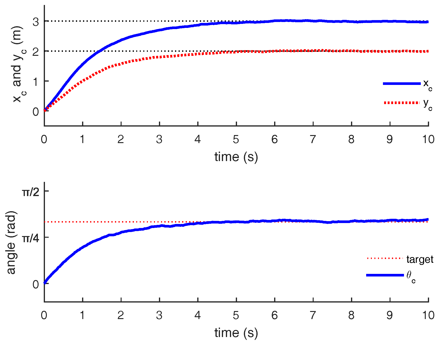
The state trajectories of the OMR in Cartesian coordinates are shown in Figure 8. Two position parameters, $x_c$ and $y_c$, are given in the upper subfigure of Figure 8. The initial position of $(x_c,y_c)$ is set to (0 m, 0 m) and the target position is set to (3 m, 2 m). The orientation angle ${\theta }_c$ of the OMR in the moving process is presented in the lower subfigure of Figure 8. The initial orientation angle is 0 rad and the target orientation angle is set to $\mathsf{\pi }$/3 rad. As shown in Figure 8, the MPC controller can steer the OMR to the target quickly and steadily.

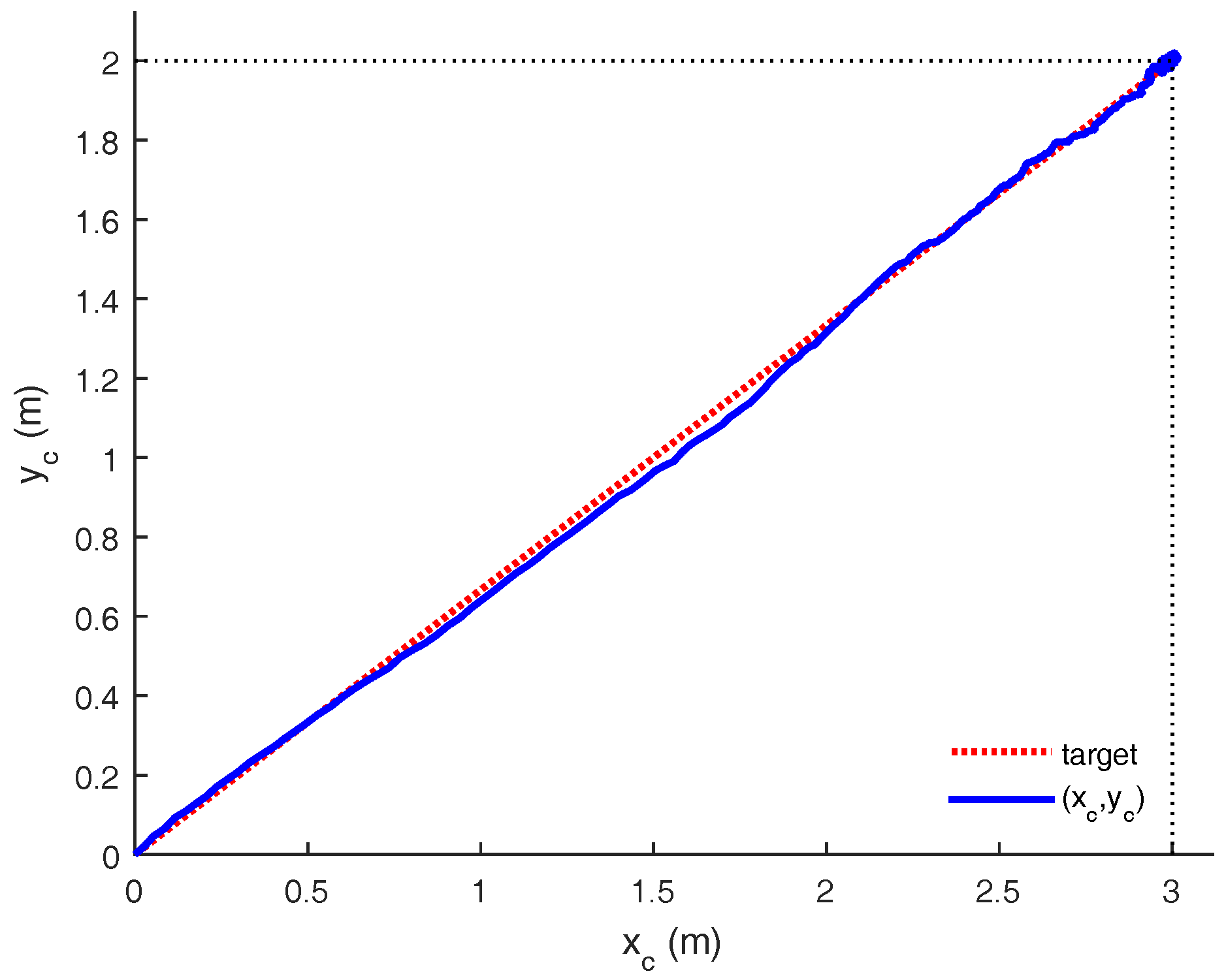
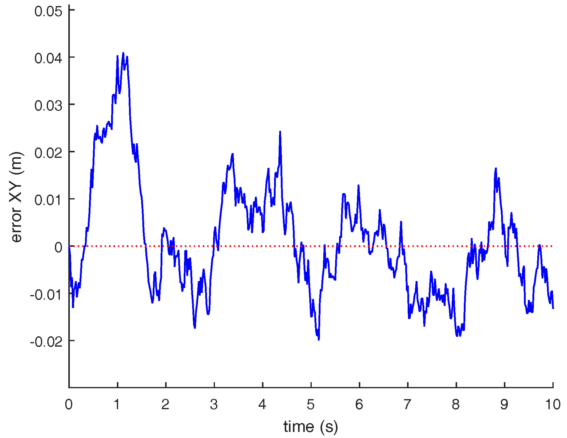
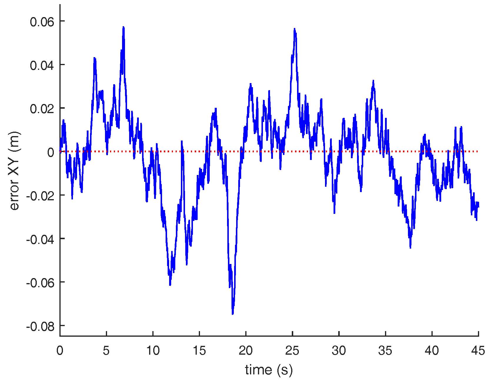
The coordinates, $\left(x_c,y_c\right)$, of the OMR in moving process are shown in Figure 9. It can be seen from this figure that the movement trajectory is very close to the target trajectory. The tracking error between the movement trajectory and the target trajectory is shown in Figure 10. The maximal tracking error is about 4 cm. From Figure 8 and Figure 10, it can be seen that the OMR moves along the predefined target trajectory to the target point, which demonstrates the effectiveness of the developed MPC algorithm.

4.2. Trajectory Tracking

In this test, the trajectory tracking of the OMR along a pulse trajectory is conducted to evaluate the performance of the proposed MPC strategy. The node parameters of the trajectory are shown in

Table 2. The node parameters of the tracking trajectory.

Index i	${\mathit{x}}_{\mathit{c}}$ (m)	${\mathit{y}}_{\mathit{c}}$ (m)	${\mathit{\theta }}_{\mathit{c}}$ (rad)
1	0	1	0
2	2	1	0
3	2	3	1.57
4	4	3	0
5	4	1	1.57
6	6	1	0

.

There are six nodes, including the starting point and end point, in the pulse trajectory. The trajectory tracking is achieved by tracking each node according to the position and target direction given in Table 2. In order to simulate the real state of the OMR, the noise is added to the output state.

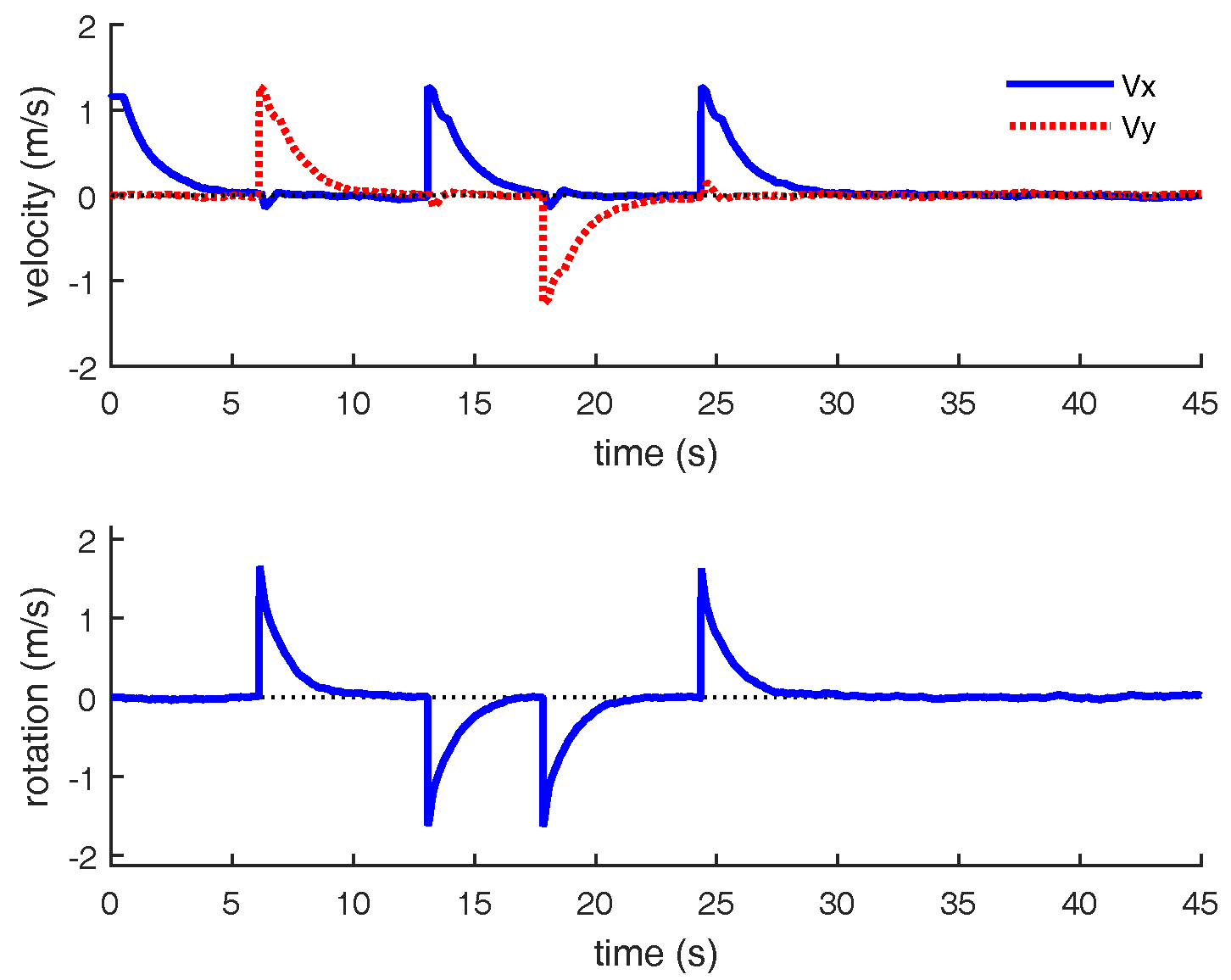
The linear velocity and angular velocity curves of the OMR in the trajectory-tracking process are shown in Figure 11. It can be seen from this figure that at each node, the axis component of linear velocity fluctuates due to steering action, but converges to zero soon.

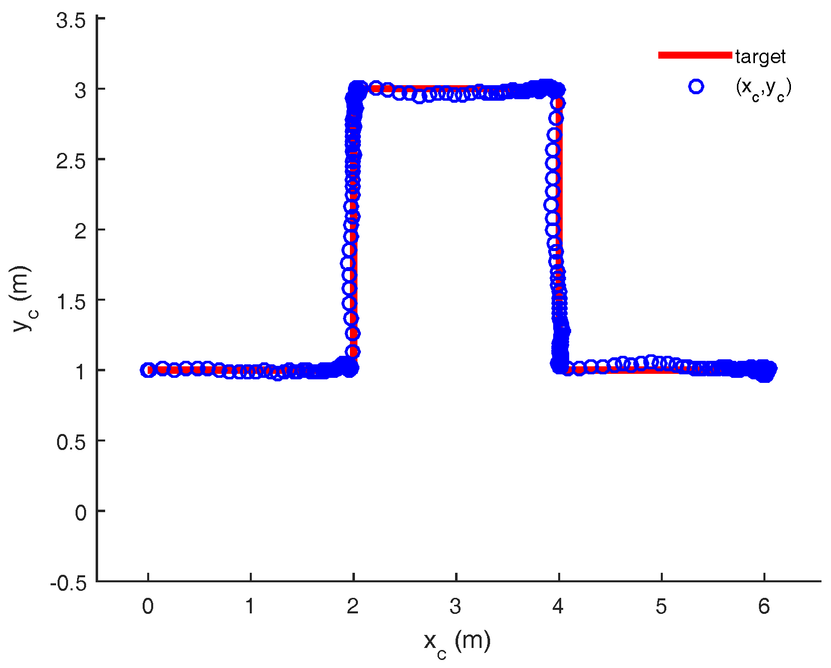
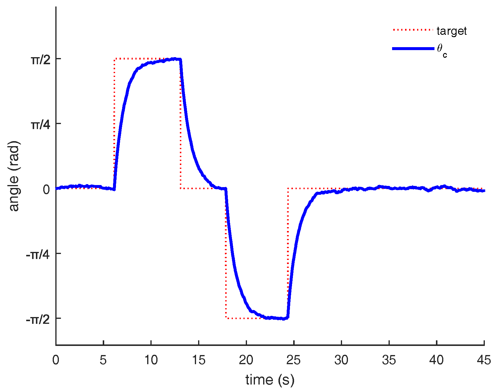
The comparisons of true and tracked trajectory and direction are shown in Figure 12 and Figure 13, respectively. As shown in these figures, the position and angle of the OMR change at the same time and the angle reaches the target faster than the position. The trajectory tracking error is presented in Figure 14. The maximal tracking error of the OMR is about 0.08 m.

The omni-directivity and flexibility of the kinematic structure of the OMR are verified through these two tests. The OMR can achieve movement of any direction without turning, which solves the problem that nonholonomic wheeled mobile robots are not flexible in real-time avoidance. In addition, the results of the first test show that the MPC algorithm can be applied in stabilization control of the robot and the target position and angle can be reached quickly and steadily.

5. Conclusions

This paper considers the trajectory tracking of an omni-directional mobile robot with three fully symmetric distribution mecanum wheels. The kinematic analysis of the OMR is conducted and the kinematic model is established. An MPC-based target-tracking motion controller with input and output state constraints is designed and guarantees the optimal solution is effective for the OMR. In addition, the advantages of the omni-directional structure compared with the traditional dual-wheeled structure with nonholonomic constraints are also discussed. The effectiveness of point stabilization and trajectory tracking of the OMR by using the designed MPC controller is demonstrated through two tests.

References

1. Zhang, X.; Fang, Y.; Sun, N. Visual servoing of mobile robots for posture stabilization: From theory to experiments. Int. J. Robust Nonlinear Control 2015, 25, 1–15. [Google Scholar] [CrossRef]
2. Li, W.; Yang, C.; Jiang, Y.; Liu, X.; Su, C. Motion Planning for Omnidirectional Wheeled Mobile Robot by Potential Field Method. J. Adv. Transport. 2017, 4961383. [Google Scholar] [CrossRef]
3. Micaelli, A.; Samson, C. Trajectory tracking for two-steering-wheels mobile robots. IFAC Proc. Vol. 1994, 14, 249–256. [Google Scholar] [CrossRef]
4. De Wit, C.C.; Sørdalen, O.J. Exponential stabilization of mobile robots with nonholonomic constraints. IEEE Trans. Autom. Control 1992, 37, 1791–1797. [Google Scholar] [CrossRef]
5. Serkies, P.J.; Szabat, K. Application of the MPC to the Position Control of the Two-Mass Drive System. IEEE Trans. Ind. Electron. 2013, 60, 3679–3688. [Google Scholar] [CrossRef]
6. Mohd Salih, J.E.; Rizon, M.; Yaacob, S.; Adom, A.H.; Mamat, M.R. Designing omni-directional mobile robot with mecanum wheel. Am. J. Appl. Sci. 2006, 3, 1831–1835. [Google Scholar] [CrossRef]
7. Asama, H.; Sato, M.; Bogoni, L.; Kaetsu, H. Development of an omni-directional mobile robot with 3 DOF decoupling drive mechanism. In Proceedings of the IEEE International Conference on Robotics and Automation, Nagoya, Japan, 21–27 May 1995; Volume 2, pp. 1925–1930. [Google Scholar]
8. Zhao, D.B.; Qiang, Y.J.; Yue, D.X. Structure and Kinematic Analysis of Omni-Directional Mobile Robots. Robot 2003, 25, 394–398. [Google Scholar]
9. Samani, H.A.; Abdollahi, A.; Ostadi, H.; Rad, S.Z. Design and Development of a Comprehensive Omni Directional Soccer Player Robot. Int. J. Adv. Robot. Syst. 2004, 1, 191–200. [Google Scholar] [CrossRef]
10. Gu, D.; Hu, H. Receding horizon tracking control of wheeled mobile robots. IEEE Trans. Control Syst. Technol. 2006, 14, 743–749. [Google Scholar]
11. Yang, S.X.; Zhu, A.; Yuan, G.; Meng, Q.H. A Bioinspired Neurodynamics-Based Approach to Tracking Control of Mobile Robots. IEEE Trans. Ind. Electron. 2012, 59, 3211–3220. [Google Scholar] [CrossRef]
12. Salaris, P.; Fontanelli, D.; Pallottino, L.; Bicchi, A. Shortest paths for a robot with nonholonomic and field-of-view constraints. IEEE Trans. Robot. 2010, 26, 269–281. [Google Scholar] [CrossRef]
13. Rashid, A.T.; Ali, A.A.; Frasca, M.; Fortuna, L. Path planning with obstacle avoidance based on visibility binary tree algorithm. Robot. Auton. Syst. 2013, 61, 1440–1449. [Google Scholar] [CrossRef]
14. Khatib, O. Real-Time Obstacle Avoidance for Manipulators and Mobile Robots. Int. J. Rob. Res. 1986, 5, 90–98. [Google Scholar] [CrossRef]
15. Kalmár-Nagy, T.; D’Andrea, R.; Ganguly, P. Near-optimal dynamic trajectory generation and control of an omnidirectional vehicle. Robot. Auton. Syst. 2004, 46, 47–64. [Google Scholar] [CrossRef]
16. Kanjanawanishkul, K.; Zell, A. Path following for an omnidirectional mobile robot based on model predictive control. In Proceedings of the IEEE International Conference on Robotics and Automation, Kobe, Japan, 12–17 May 2009; pp. 3341–3346. [Google Scholar]
17. Huang, H.C.; Tsai, C.C. Adaptive Trajectory Tracking and Stabilization for Omnidirectional Mobile Robot with Dynamic Effect and Uncertainties. IFAC Proc. Vol. 2008, 41, 5383–5388. [Google Scholar] [CrossRef]
18. Ortíz, J.M.; Olivares, M. Trajectory Tracking Control of an Omnidirectional Mobile Robot Based on MPC. In Proceedings of the IEEE Fourth Latin American Robotics Symposium (Lars 2007), Monterrey, Mexico, 8–9 November 2007. [Google Scholar]
19. Li, Z.; Yang, C.; Su, C.Y.; Deng, J.; Zhang, W. Vision-Based Model Predictive Control for Steering of a Nonholonomic Mobile Robot. IEEE Trans. Control Syst. Technol. 2016, 24, 553–564. [Google Scholar] [CrossRef]
20. Klančar, G.; Škrjanc, I. Tracking-error model-based predictive control for mobile robots in real time. Robot. Auton. Syst. 2007, 55, 460–469. [Google Scholar] [CrossRef]
21. Araújo, H.X.; Conceição, A.G.S.; Oliveira, G.H.C.; Pitanga, J. Model Predictive Control based on LMIs Applied to an Omni-Directional Mobile Robot. IFAC Proc. Vol. 2011, 44, 8171–8176. [Google Scholar] [CrossRef]
22. Kanjanawanishkul, K. MPC-Based Path Following Control of an Omnidirectional Mobile Robot with Consideration of Robot Constraints. Adv. Electr. Electron. Eng. 2015, 13, 54–63. [Google Scholar] [CrossRef]
23. Holmberg, R.; Khatib, O. Development and Control of a Holonomic Mobile Robot for Mobile Manipulation Tasks. Int. J. Robot. Res. 1999, 19, 1066–1074. [Google Scholar] [CrossRef]
Figure 1. The structure of the mecanum wheel.
Applsci 08 00231 g001
Figure 2. The omni-directional mobile robot (OMR) structure diagram.
Applsci 08 00231 g002
Figure 3. The wheel location and pose in the platform center.
Applsci 08 00231 g003
Figure 4. The wheel location and pose in the platform center.
Applsci 08 00231 g004
Figure 5. The state of the OMR in Cartesian coordinates.
Applsci 08 00231 g005
Figure 6. Three-wheeled structure layout of the platform.
Applsci 08 00231 g006
Figure 7. The velocity inputs of three mecanum wheels.
Applsci 08 00231 g007
Figure 8. The state trajectories of the OMR in Cartesian coordinates.
Applsci 08 00231 g008
Figure 9. The trajectory coordinates of the OMR.
Applsci 08 00231 g009
Figure 10. The tracking error.
Applsci 08 00231 g010
Figure 11. The line velocity and angular velocity of the OMR.
Applsci 08 00231 g011
Figure 12. The real trajectory of the OMR.
Applsci 08 00231 g012
Figure 13. The orientation of the OMR.
Applsci 08 00231 g013
Figure 14. The trajectory offset of the OMR.
Applsci 08 00231 g014