Abstract
To feasibly achieve economical and satisfactory robust velocity tracking of an induction machine (IM), we propose an Arduino-implemented intelligent speed controller. Because a voltage/frequency controlled IM framework is simple and well suited for being controlled by the proposed speed controller, it is adopted herein. Taking into account easy implementation and good performance, we design the controller using a modified Ziegler-Nichols PID (modified Z-N PID) and a fuzzy logic controller (FLC). The modified Z-N PID and the FLC are connected in tandem. The latter is designed based on the output signal of the former for adaptively yielding adequate torque commands. Experimental results of IM velocity tracking controlled by our PC-based and Arduino-based speed controllers consistently show that the proposed design scheme can yield remarkable tracking performance and robustness. In addition, it is demonstrated that the proposed Arduino-implemented controller is not only viable but also effective in terms of cost, size and tracking performance.
1. Introduction
Induction machine (IM) drives [1,2] have been widely utilized in motion control applications such as the speed control of a pump, or a machine tool, or an electric vehicle, etc. (e.g., [3,4]). To achieve high servo quality, many studies (e.g., [5,6]) have been focused on the speed control of a direct-field-oriented (DFO) IM. However, additional design efforts for decoupling the torque and flux control of a DFO IM are required. Additionally, the decoupling control is vulnerable to adverse load disturbances and parameter variations which can severely degrade tracking performance. In comparison, the speed controller design for a voltage/frequency (V/f) controlled IM is generally much simpler than that for a DFO IM. Accordingly, this paper adopts a V/f controlled IM framework for speed control.
In motion control applications, it is desirable that a controlled IM should closely follow a reference speed trajectory in situations with or without torque disturbances. Though the system stability may be guaranteed by using the conventional proportional-integral (PI) or proportional-integral-derivative (PID) speed controllers (e.g., [7]) with well-chosen parameter values, the robustness to abrupt load changes in the motor may not be improved. This difficulty may be overcome by using a model-based predictive control strategy (e.g., [5,6,8]), an adaptive backstepping method (e.g., [9]), a descriptor approach (e.g., [10]), a composite nonlinear feedback control scheme (e.g., [11]), or a output-feedback control method (e.g., [12]). However, the control performance relies on how well the system is described by the model. Accordingly, the incorporation of machine intelligence into the control of IM drives has been widely used as a viable alternative for improving the system stability, performance and robustness. Specifically, intelligent controllers for IM drives have been proposed based on fuzzy logic (e.g., [13,14,15]) or neural networks (e.g., [16]) or neuro-fuzzy inferences (e.g., [17,18,19]) or a particle swarm optimization algorithm (e.g., [3]). Based on the use of a fuzzy controller for adaptively adjusting PID parameter values, a fuzzy P+ID controller in [20], a fuzzy PI self-tuning controller in [21,22,23] and a fuzzy self-tuning fuzzy PID controller in [24,25] may also be employed. In addition, a fuzzy model-based predictive control strategy (e.g., [26]) may be utilized. Nevertheless, the aforementioned controller structures did not investigate a control scheme composed of a fixed-gain PI or PID in combination with a fuzzy-logic controller (FLC). Thus, a Ziegler-Nichols (Z-N) PID (e.g., [27]) in tandem with a FLC was proposed in [28] for the control of a DFO IM. Unlike best trial-and-error PI or PID controllers, the foregoing intelligent controllers can adaptively mitigate the adverse effects of torque disturbances and achieve desirable performance.
The first objective of this paper is to present an intelligent control scheme which has simple design and satisfactory performance for robust speed control of a V/f controlled IM. In this regard, we propose a modified Z-N PID+Fuzzy controller, which consists of a fixed-gain modified Z-N PID in [29] together with an FLC. Our proposed approach is distinct from other schemes (e.g., [30,31,32]). The modified Z-N PID is adopted because it can outperform the Z-N PID. Like the Z-N PID+Fuzzy in [28], the modified Z-N PID and the FLC of the proposed controller are connected in tandem. We design an adequate FLC, distinct from the FLC in [28,33] in membership functions, based on the output signal of the modified Z-N PID. The FLC gives adequate torque commands which in turn yield appropriate stator frequency commands for controlling the speed of the IM. Meanwhile, the FLC does not tune PID parameter values.
The second objective of this paper is to feasibly achieve low-cost control implementation. In this regard, we propose an Arduino rather than a Field-Programmable Gate Array (FPGA) (e.g., [34,35,36,37]) for the implementation of the proposed speed controller. Our main reasons for this choice are given as follows. Firstly, the use of a software programming language to develop a control scheme is simpler and more user-friendly than that of a hardware description language. Secondly, the use of an Arduino may save more computational resources. Thirdly, an Arduino is much more economical than an FPGA.
The advantages of the proposed control scheme for speed tracking of a V/f controlled Nikki Denso NA21-3F 0.14-hp squirrel-cage IM are evaluated. Despite various motor horsepower, induction motors have a similar internal functional structure. Thus, a control design methodology for the 0.14-hp induction motor is in general applicable to the control design of induction motors with larger horsepower. Experiments with/without load torque disturbances are performed by PC-based and Arduino-based control. The PC and the Arduino plus the circuits which we design cost around US $600.00 and US $32.00, respectively. The experimental results consistently demonstrate that the proposed scheme can noticeably outperform several control schemes such as a Z-N PID and a modified Z-N PID in speed tracking and robustness. It is noted that the Arduino-implemented modified Z-N PID+Fuzzy for speed control of the V/f controlled IM yields slightly higher tracking errors than the PC-based modified Z-N PID+Fuzzy. Nevertheless, the Arduino-implemented controller is preferable in consideration of price, size, and robust tracking performance.
The outline of this paper is as follows. Section 2 describes the framework for speed control of a V/f controlled IM. Section 3 presents the proposed intelligent control method. The experimental setups are described in Section 4. The experimental results of PC- and Arduino-implementation of the proposed control design method and other schemes are provided. Conclusions are given in Section 5.
2. System Description
For the velocity control of the V/f controlled IM, the system mainly consists of three parts: IM, V/f controller and speed controller. The block diagram of the closed-loop system structure is shown in Figure 1 (cf. Figure 7.18 in [2]).
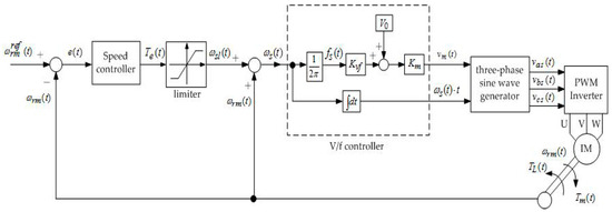
Figure 1.
Functional structure of speed control of a V/f controlled induction machine (IM).
For the IM, its input phase voltages are transformed from three-phase stator rms voltage inputs , and , which are generated by the outputs of the V/f controller via a three-phase sine wave generator as follows:
where and denote the supply voltage and the electrical angular velocity, respectively. A simplified IM model represented by the input–output relation between the electromagnetic torque and the mechanical angular velocity (rad/s) can be written as
where represents an external load torque; and stand for the rotor inertia and the coefficient of viscous damping, respectively.
For the V/f controller, its inputs are and , which stand for a stator frequency command (Hz) and an offset voltage to counter the stator resistive voltage drop, respectively. The stator frequency command is set as
where is the slip speed. The outputs of the V/f controller are and . The input and output relations are given by
and
where is a constant ratio between the stator-phase voltage and the stator frequency, and is a constant gain.
For the speed controller, its input is the difference error
and its output is the control command where denotes the reference speed (rad/s). The input of the limiter is and its output is given by
where denotes the rotor resistance; and stand for the stator and rotor inductances, respectively.
3. Proposed Intelligent Speed Controller
In this section, we present the development of the proposed intelligent speed controller, modified Z-N PID+Fuzzy, depicted in Figure 2. The proposed speed controller consists of a modified Z-N PID in conjunction with a fuzzy logic controller (FLC). The role of the FLC is to adaptively adjust the output of the modified Z-N PID into an adequate control command .
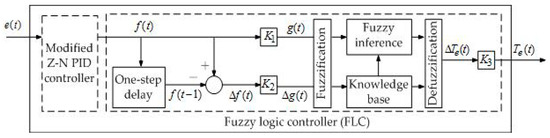
Figure 2.
Functional structure of the proposed speed controller.
3.1. Development of a Modified Z-N PID Controller
To yield a Z-N PID and a modified Z-N PID for the system depicted in Figure 1, we initially adopt the design steps in [29] as a guideline. To begin with, we employ a linear proportional speed controller in Figure 1 with zero external load torque. A step input is applied, and the proportional gain of the speed controller is increased until the system reaches the stability limit so as to acquire the time of the critical oscillation and the critical proportional gain . The Z-N PID controller can be obtained using , and the ‘rule of thumb’ formula in [27]. Next, the stability margin of the system can be further improved by utilizing the modified Z-N PID speed controller to move the point with a distance to the origin and the phase −180° on the Nyquist curve to a specified new position with a distance satisfying and a phase satisfying −180° < < −90°. The modified Z-N PID speed controller is given by
where the proportional gain
the integral time
and the derivative time
3.2. Development of an FLC
The FLC consists of fuzzification and defuzzification. It is noted that we take into account not only but also its one-step difference variation . This is to make the FLC adaptive to the PID output and its variation. We employ the proportional gains of and , i.e., and as inputs of membership functions. In the fuzzification process, trapezoidal-shape and triangular-shape membership functions are used since are used they are computationally simple and straightforward to design and interpret membership grades. Conventionally, a membership function is trapezoidal-shape for both intervals and while it is triangular-shape for any finite interval. For any , where stands for the interval , the related linguistic value for their membership functions is ‘N’. For any , where denotes the interval , the related linguistic value for their membership functions is ‘P’. For any , where represents a given interval , the related linguistic value for its membership function is ‘Z’. Since is a variation value, we set the interval not larger than for its membership function to be triangular-shape. Certainly, the value 0.25 is set heuristically and can be replaced by other positive value less than 1. For any, , where represents the interval , the related linguistic value for its membership function is ‘Z’. Accordingly, the two membership functions are given by
Correspondingly, the membership functions in Equations (14)–(16) and (17)–(19) are depicted in Figure 3.
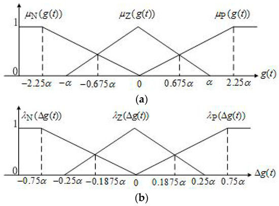
Figure 3.
Membership functions. (a) Membership function for input ; (b) Membership function for input .
The fuzzy inference engine is derived from the input fuzzy sets together with expert’s experience. It makes decisions by using adequate IF–THEN rules in the knowledge base as well as yields an implied output fuzzy set . In this study, we use the proposed IF–THEN fuzzy rule base in Figure 4 and given by
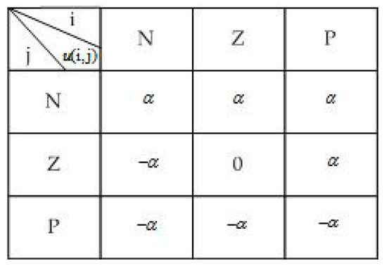
Figure 4.
Fuzzy rule base.
In addition, the Mamdani-type min operation is adopted for fuzzy inferences.
In the defuzzification process, the implied output fuzzy set is mapped into a crisp output by using the ‘center of mass’ defuzzification method. Specifically,
where the fuzzification function is given by
The FLC yields the control command
Based on the input membership functions Equations (14)–(16) and (17)–(19), the fuzzy rule base Equation (20) and the defuzzification Equations (21) and (22), we can divide the operation area into 36 regions shown in Figure 5. Accordingly, we have
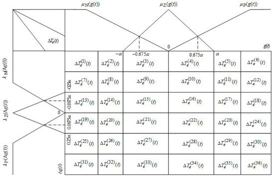
Figure 5.
Thirty-six distinct regions resulting from the min operation.
In the following, we illustrate that the command can be adaptively adjusted by tuning gains in the FLC. We take the generation of for yielding as an illustrative example. In the region 14 of Figure 5, we have and . According to Figure 4 and Figure 5, we only have to consider two cases: Case 1, and ; and Case 2, and .
- Case 1. This yields . We have since . Moreover, since . So, we get
- Case 2. This yields . We have since . Moreover, since . So, we get
Based on Equation (21), we get
Since we have , , Equation (28) and , it is apparent that adequate control commands can be obtained adaptively by intelligently tuning gains , and as well as the value .
4. Experimental Study
The experimental tests are performed on a Nikki Denso NA21-3F 0.14-hp induction motor. We carry out various PC- and Arduino-implemented experimental tests on the performance of the proposed method and other controller schemes. The experimental results consistently confirm that the proposed modified Z-N PID+Fuzzy method can give noticeable robustness and improvements over other schemes tested. In addition, it is demonstrated that the proposed low-cost Arduino-implemented control scheme can feasibly and effectively yield satisfactory robust performance though it gives slightly higher tracking errors than the proposed PC-based counterpart.
4.1. Experimental Setup
For the V/f controller in Figure 1, the parameter values are set as follows: , and In accordance with the information in the specification and instruction manual of the Nikki Denso NA21-3F 0.14-hp induction motor, the motor parameter values in Equations (4) and (9) are given by (kg·cm·s2), (g·cm/rpm), and .
To obtain various speed controllers, we use the Matlab/Simulink software and the system functional structure in Figure 1 to develop a computer simulation model in which the three-phase induction motor is used with parameters provided as above, and no external load torque is applied. To obtain a Z-N PID and a modified Z-N PID, we first employ a linear proportional speed controller in the simulation model. Next, a step input is applied, and the proportional gain is adjusted until the system reaches the stability limit. However, no critical oscillation takes place at the system output; only system output divergence can occur. Therefore, we adapt the design steps described in [29] and in Section 3.1 to obtain the critical gain and the critical time period. In practice, we increase the gain, and get the approximate critical gain with which the system diverges immediately at the approximate time 0.049 s. Then, we take . This together with the formula in [27], the Z-N PID is given by . Moreover, based on Equations (10)–(12) with and = −135°, the modified Z-N PID is given by .
To obtain a desirable FLC for the modified Z-N PID+Fuzzy, we first heuristically set the parameter values and . Next, we use Equations (14)–(23) and adjust the values of the parameters and until closed-loop system responses of the Matlab/Simulink computer simulation model under no torque disturbance are satisfactory. As a result, we get and .
The experimental tests are carried out using the PC-based and the Arduino-based control schemes. In addition, all speed controllers obtained above are employed in the experimental tests.
Figure 6 shows the block diagram of the functional implementation structure of the Matlab/Simulink on the PC and the Arduino. The details of those modules and connections can be referred to in Figure 1 and Equations (1)–(3), (5)–(10) and (14)–(23).
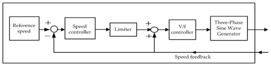
Figure 6.
Functional implementation structure of PC (Matlab/Simulink) and Arduino.
Figure 7 displays the PC-implemented induction motor control system. The real-time implementation of the control system employs the MRC-6810 AD/DA servo control card as the interface between software and hardware. The MRC-6810 card resides in the PC and is directly connected to the block diagram of the multi-channel AD/DA converter of the Matlab/Simulink on the PC to send and receive signals. The voltage drive circuit residing in PC yields adequate voltage signals based on signal outputs from the Matlab/Simulink on the PC to the PWM inverter via the D/A channel of the MRC-6810 card. The motor speed is sensed by the speed encoder mounted on the rotor shaft. The encoder produces a pulse signal, and then the frequency (F) of the pulse signal is converted into a voltage signal (V) by the DSP TMS320F240. The voltage signal is fed back to the Matlab/Simulink on the PC via the A/D channel of the MRC-6810 card to complete the speed feedback action.
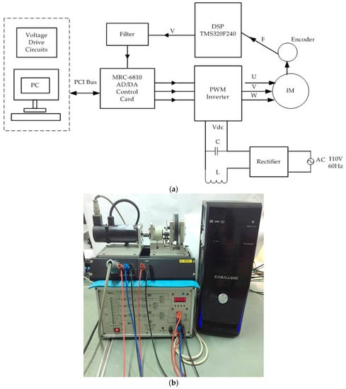
Figure 7.
PC-implemented speed tracking of the V/f controlled IM. (a) Schematic diagram; (b) Realistic experimental setup.
Figure 8 shows the Arduino-implemented induction motor control system. The Arduino model UNO—a single-chip microcomputer—is used. It provides the simplicity of operating its I/O interface, and a user-friendly Java programming development environment. It has the built-in A/D operation but has no D/A function. Furthermore, the operating ranges of its input and output voltages are different from those of the output voltages of the DSP TMS320F240 as well as those of input voltages of the PWM inverter. Thus, we design adequate external circuits to integrate the Arduino into the induction motor control system. First, a voltage booster circuit is designed and utilized for increasing analog feedback voltage signals from the DSP TMS320F240 with a range of ±1.5 V to reach the voltage range of zero to five volts as the Arduino input. Then zero to five volt analog signals are converted to digital signals via the Arduino’s built-in A/D converter. Second, since the Arduino has no built-in D/A converter, the 12-bit DAC128S085 chip is used. Moreover, a voltage amplifier circuit is designed and utilized for increasing analog signal outputs from the D/A converter to the voltage range of −10 V to +10 V as the PWM inverter inputs.
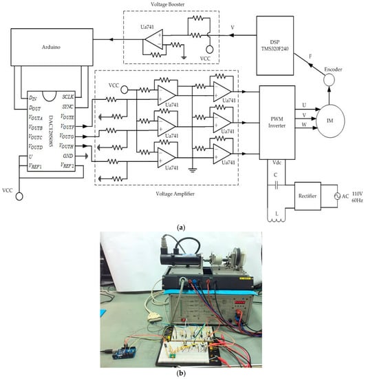
Figure 8.
Arduino-implemented speed tracking of the V/f controlled IM. (a) Schematic diagram; (b) Realistic experimental setup.
4.2. Experimental Results
In the sequel, the proposed modified Z-N PID+Fuzzy, the modified Z-N PID and the Z-N PID are abbreviated as Modified Z-N+Fuzzy, Modified Z-N and Z-N, respectively.
In the experimental tests, we use a cycle of the reference speed command. The reference speed is increased from 0 rpm to 900 rpm at 4.25 s and then starts decreasing from 900 rpm at 8.25 s to −900 rpm at 16.25 s and subsequently, starts increasing from −900 rpm at 20.25 s to 0 rpm at 24.25 s. In addition, test cases with and without sudden load change are as follows:
- Case A. No external load torque is applied to the shaft;
- Case B. An external load torque of 1.1 Nm is suddenly applied to the shaft at 5 s;
- Case C. An external load torque of 1.1 Nm is suddenly applied to the shaft at 18 s.
For the PC-based and the Arduino-based experiments, we obtain the instantaneous velocity tracking performance of the V/f controlled IM using Modified Z-N+Fuzzy, Modified Z-N and Z-N. We also obtain the root-mean-square-errors (RMSE) of each method based on the average over 100 runs for the PC-based experiments. In addition, numerical comparisons of robust tracking performance with and without sudden load changes can be acquired based on maximum speed error (%) between 4.2 s and 8.25 s as well as that between 16.25 s and 20.25 s). The settling time is also taken into account (i.e., when the reference speed 900 rpm/or −900 rpm, after the motor speed reaches 900 rpm/or −900 rpm, the last time that the motor speed lies between 855 rpm and 945 rpm/or −855 rpm). No steady state error is considered since the command speed is time-varying.
The experimental results consistently confirm that the proposed Modified Z-N+Fuzzy is the best among controllers tested. The Arduino-implemented Modified Z-N+Fuzzy for the V/f controlled IM speed tracking generally yields higher tracking errors (e.g., larger maximum speed error) and longer settling time than its PC-based counterpart. Even so, it is a favorable choice when the tradeoff between price, size and robust tracking performance is taken into account.
4.2.1. PC-Based IM Speed Tracking
Experimental results for the Case A are shown in Figure 9 and Table 1. The instantaneous and the RMSE performance in Figure 9 show that the proposed Modified Z-N+Fuzzy can track the command speed slightly better than other controllers. Table 1 shows that the proposed Modified Z-N+Fuzzy slightly outperforms other controllers under no sudden load change in terms of smaller maximum speed error and quicker settling time.
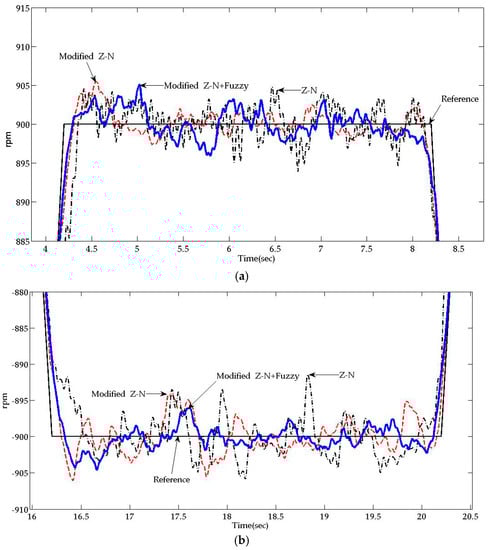
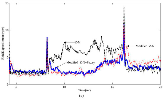
Figure 9.
Velocity tracking of the V/f controlled induction motor for Case A using various PC-implemented speed controllers. (a) Instantaneous performance comparison during 4–8.5 s; (b) Instantaneous performance comparison during 16–20.5 s; (c) RMSE performance comparison during 4.2–20.5 s.

Table 1.
Numerical robust tracking performance comparison based on Figure 9.
Experimental results for the Case B and those for the Case C are shown in Figure 10 and Figure 11, respectively. Figure 10 and Figure 11 show that the proposed Modified Z-N+Fuzzy is more robust than the other controllers since it results in both smaller velocity tracking errors and quicker system response reversion to normal when a load torque disturbance suddenly takes place. Moreover, Table 2 and Table 3, show that the proposed Modified Z-N+Fuzzy has smaller maximum speed error and shorter settling time under a sudden load change.
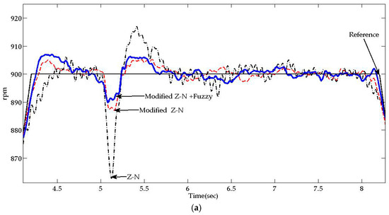
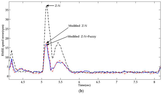
Figure 10.
Velocity tracking of the V/f controlled induction motor for Case B using various PC-implemented speed controllers. (a) Instantaneous performance comparison during 4–8.5 s; (b) RMSE performance comparison during 4–8.5 s.
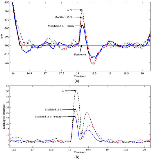
Figure 11.
Velocity tracking of the V/f controlled induction motor for Case C using various PC-implemented speed controllers. (a) Instantaneous performance comparison during 16.25–20.25 s; (b) RMSE performance comparison during 16.25–20.25 s.
Table 2.
Numerical robust tracking performance comparison based on Figure 10.
Table 3.
Numerical robust tracking performance comparison based on Figure 11.
4.2.2. Arduino-Based IM Speed Tracking
Unlike a PC, the Arduino is far cheaper but it does not have sufficient memory for storing a large amount of data. As a result, Arduino-based experimental tests can only yield instantaneous performance. No RMSE performance can be acquired.
For the case with no sudden load change, the experimental results are shown in Figure 12 and Table 4. Figure 12 displays that the Modified Z-N+Fuzzy yields slightly smaller velocity tracking errors than other controllers. Table 4 indicates that the proposed Modified Z-N+Fuzzy achieves slightly smaller maximum speed error and settling time. They are consistent with the conclusion resulting from the PC-based experimental outcomes in Figure 9 and Table 1. For the cases with sudden load changes, the experimental outcomes are shown in Figure 13 and Figure 14 and Table 5 and Table 6. They show that the Modified Z-N+Fuzzy is much more robust than the other controllers because it yields much smaller peak tracking error and faster settling time when a load torque disturbance suddenly takes place. This is consistent with the conclusion drawn from Figure 10 and Figure 11 and Table 2 and Table 3.
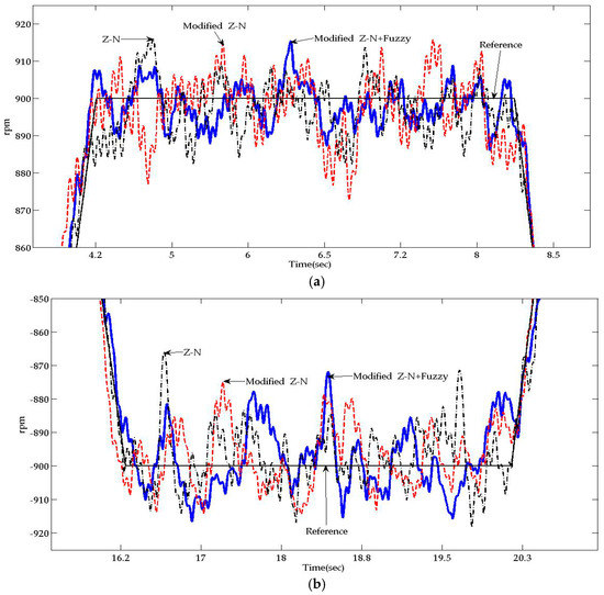
Figure 12.
Velocity tracking of the V/f controlled Induction Motor for Case A using various Arduino-implemented speed controllers. Instantaneous performance comparison during (a) 4–8.5 s and (b) 16–20.5 s.
Table 4.
Numerical robust tracking performance comparison based on Figure 12.
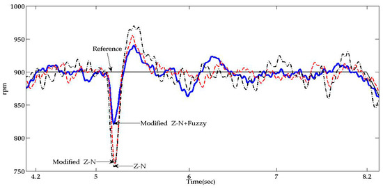
Figure 13.
Velocity tracking of the V/f controlled Induction Motor for Case B using various Arduino-implemented speed controllers. Instantaneous performance comparison during 4–8.25 s.
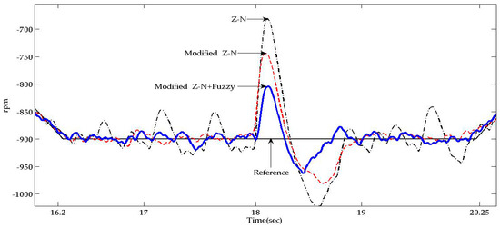
Figure 14.
Velocity tracking of the V/f controlled Induction Motor for Case C using various Arduino-implemented speed controllers. Instantaneous performance comparison during 16–20.35 s.
Table 5.
Numerical robust tracking performance comparison based on Figure 13.
Table 6.
Numerical robust tracking performance comparison based on Figure 14.
5. Conclusions
In this paper, we have presented the development of the Arduino-based modified Z-N PID+Fuzzy controller design scheme for controlling the speed of a V/f controlled IM effectively and robustly. Moreover, the proposed controller and other control schemes have been implemented using a PC and the Arduino for speed tracking of a Nikki Denso NA21-3F 0.14-hp IM. The experimental results have consistently confirmed that the proposed modified Z-N PID+Fuzzy controller remarkably outperforms other controllers tested in view of tracking performance with or without load torque disturbances. The main factor for the superior performance of the proposed controller is that the combined advantages of the modified Z-N PID and fuzzy inferences can adaptively enhance the system stability and performance.
As the Arduino has less memory than a PC, it is not surprising that the Arduino-implemented modified Z-N+Fuzzy controller generally yields higher tracking errors and longer settling time than its PC-based counterpart. Despite this, the Arduino implementation is cost-effective and favorable in consideration of a compromise between price and tracking performance. In our future research, we will develop other low-cost and efficient methods for improving the Arduino-implemented modified Z-N PID+Fuzzy controller.
Acknowledgments
The work of Tan-Jan Ho was partially supported by Chung Yuan Christian University, Taiwan. The authors thank two of the reviewers for major constructive comments and suggestions, which help to improve the presentation of the paper.
Author Contributions
Tan-Jan Ho initiated the research problem, conceived the proposed method and implementation, and wrote the paper; Chun-Hao Chang performed the experimental design and tests, and took photos; Chun-Hao Chang and Tan-Jan Ho analyzed the data.
Conflicts of Interest
The authors declare no conflict of interest.
References
- Blaschke, F. The principle of field orientation as applied to the new transvector closed-loop control system for rotating-field machines. Siemens Rev. 1972, 39, 217–220. [Google Scholar]
- Krishnan, R. Electric Motor Drive: Modeling, Analysis and Control; Prentice Hall Inc.: Upper Saddle River, NJ, USA, 2001. [Google Scholar]
- Zhang, Z.; Xu, H.; Xu, L.; Heilman, L.E. Sensorless direct field-oriented control of three-phase induction motors based on sliding mode for washing-machine drive applications. IEEE Trans. Ind. Appl. 2006, 42, 694–701. [Google Scholar] [CrossRef]
- Elwer, A.S. A novel technique for tuning PI-controllers in induction motor drive systems for electric vehicle applications. J. Power Electron. 2006, 6, 322–329. [Google Scholar]
- Santana, E.S.; Bim, E.; Amaral, W.C. A predictive algorithm for controlling speed and rotor flux of induction motor. IEEE Trans. Ind. Electron. 2008, 55, 717–725. [Google Scholar] [CrossRef]
- Egiguren, P.A.; Caramazana, O.B.; Etxeberria, J.A.C. TNC-Generalized Predictive Speed Control of Induction Motor Drives. In Proceedings of the 37th Annual Conference of IEEE Industrial Electronics, Melbourne, Australia, 7–10 November 2011. [Google Scholar]
- Kuo, B.C.; Golnaraghi, M.F. Automatic Control Systems; John Wiley & Sons: Hoboken, NJ, USA, 2003. [Google Scholar]
- Thomas, J.; Hansson, A. Speed tracking of a linear induction motor-enumerative nonlinear model predictive control. IEEE Trans. Control Syst. Technol. 2013, 21, 1956–1962. [Google Scholar] [CrossRef]
- Zaafouri, A.; Regaya, C.B.; Azza, H.B.; Châari, A. DSP-based adaptive backstepping using the tracking errors for high-performance sensorless speed control of induction motor drive. ISA Trans. 2016, 60, 333–347. [Google Scholar] [CrossRef] [PubMed]
- Aouaouda, S.; Chadli, M.; Boukhnifer, M.; Karimi, H.R. Robust fault tolerant tracking controller design for vehicle dynamics: A descriptor approach. Mechatronics 2015, 30, 316–326. [Google Scholar] [CrossRef]
- Hu, C.; Wang, R.; Yan, F.; Chen, N. Robust composite nonlinear feedback path-following control for underactuated surface vessels with desired-heading amendment. IEEE Trans. Ind. Electron. 2016, 63, 6386–6394. [Google Scholar] [CrossRef]
- Hu, C.; Jing, H.; Wang, R.; Yan, F.; Chadli, M. Robust H∞ output-feedback control for path following of autonomous ground vehicles. Mech. Syst. Signal Process. 2016, 70, 414–427. [Google Scholar] [CrossRef]
- Brrero, F.A.; Gonzalez, A.; Torralba, A.; Galvan, E.; Franquelo, L.G. Speed control of induction motors using a novel fuzzy sliding-mode structure. IEEE Trans. Fuzzy Syst. 2002, 10, 375–383. [Google Scholar] [CrossRef]
- Heber, B.; Xu, L.; Tang, Y. Fuzzy logic enhanced speed control of an indirect field-oriented induction machine drive. IEEE Trans. Power Electron. 1997, 12, 772–778. [Google Scholar] [CrossRef]
- Rafa, S.; Larabi, A.; Barazane, L.; Manceur, M.; Essounbouli, N.; Hamzaoui, A. Implementation of a new fuzzy vector control of induction motor. ISA Trans. 2014, 53, 744–754. [Google Scholar] [CrossRef] [PubMed]
- Wai, R.J.; Chang, H.H. Backstepping wavelet neural network control for indirect field-oriented induction motor drives. IEEE Trans. Neural Netw. 2004, 15, 367–382. [Google Scholar] [CrossRef] [PubMed]
- Uddin, M.N.; Wen, H. Development of a self-tuned neuro-fuzzy controller for induction motor drives. IEEE Trans. Ind. Appl. 2007, 43, 1108–1116. [Google Scholar] [CrossRef]
- Hafeez, M.; Uddin, M.N.; Rahim, N.A. Self-tuned NFC and adaptive torque hysteresis-based DTC scheme for IM drive. IEEE Trans. Ind. Appl. 2014, 50, 1410–1420. [Google Scholar] [CrossRef]
- Karithik, M.; Reddy, M.K. Speed control of induction motor by using self-tuned neuro fuzzy logic controller. Int. J. Innov. Technol. 2015, 3, 358–364. [Google Scholar]
- Li, W. Design of a hybrid fuzzy logic proportional plus conventional integral-derivative controller. IEEE Trans. Fuzzy Syst. 1998, 6, 449–463. [Google Scholar] [CrossRef]
- Lokriti, A.; Salhi, I.; Doubabi, S.; Zidani, Y. Induction motor speed drive improvement using fuzzy IP-self-tuning controller, a real time implementation. ISA Trans. 2013, 52, 406–417. [Google Scholar] [CrossRef] [PubMed]
- Daya, J.L.F.; Subbiah, J.; Sanjeevikumar, P. Robust speed control of an induction motor drive using wavelet–fuzzy based self-tuning multiresolution controller. Int. J. Comput. Intell. Syst. 2013, 6, 724–738. [Google Scholar] [CrossRef]
- Menghal, P.M.; Laxmi, A.J. Fuzzy based real time control of induction motor drive. Procedia Comput. Sci. 2016, 85, 228–235. [Google Scholar] [CrossRef]
- Kumar, R.A.; Daya, J.L.F. A Novel Self-Tuning Fuzzy Based PID Controller for Speed Control of Induction Motor Drive. In Proceedings of the International Conference on Control Communication and Computing, Thiruvananthapuram, India, 13–15 December 2013. [Google Scholar]
- Devi, K.; Gautam, S.; Nagaria, D. Speed control of 3-phase induction motor using self-tuning fuzzy PID controller and conventional PID controller. Int. J. Inf. Comput. Technol. 2014, 4, 1185–1193. [Google Scholar]
- Yang, T.; Qiu, W.; Ma, Y.; Chadli, M.; Zhang, L. Fuzzy model-based predictive control of dissolved oxygen in activated sludge processes. Neurocomputing 2014, 136, 88–95. [Google Scholar] [CrossRef]
- Van Doren, V. Auto-tuning control using Ziegler-Nichols. Control Eng. 2006, 53, 66–71. [Google Scholar]
- Ho, T.J.; Yeh, L.Y. Design of a Hybrid PID Plus Fuzzy Controller for Speed Control of Induction Motors. In Proceedings of the 2010 IEEE Conference on Industrial Electronics and Applications, Taichung, Taiwan, 15–17 June 2010. [Google Scholar]
- Olsson, M. Simulation Comparison of Auto-Tuning Methods for PID Control; Linköping University Electronic Press: Linköping, Sweden, 2008. [Google Scholar]
- Suzuki, K.; Saito, S.; Kudor, T.; Tanaka, A.; Andoh, Y. Stability Improvement of V/F Controlled Large Capacity Voltage-Source Inverter Fed Induction Motor. In Proceedings of the 41st IEEE Conference on Industry Applications, Tampa, FL, USA, 8–12 October 2006. [Google Scholar]
- Yang, R.; Chen, W.; Yu, Y.; Xu, D. Stability Improvement of V/F Controlled Induction Motor Drive Systems Based on Reactive Current Compensation. In Proceedings of the 2008 IEEE Conference on Electrical Machines and Systems, Wuhan, China, 17–20 October 2008. [Google Scholar]
- Amudhavalli, D.; Narendran, L. Speed Control of an Induction Motor by V/F Method Using an Improved Z Source Inverter. In Proceedings of the 2012 IEEE Conference on Emerging Trends in Electrical Engineering and Energy Management, Tamil Nadu, India, 13–15 December 2012. [Google Scholar]
- Ho, T.J.; Chang, C.H. Effective Speed Tracking of Induction Motors Using Microcontroller-Based Intelligent Control. In Proceedings of the 2017 IEEE International Conference on Applied System Innovation, Sapporo, Japan, 13–17 May 2017. [Google Scholar]
- Lin, F.J.; Wang, D.H.; Huang, P.K. FPGA-based fuzzy sliding-mode control for a linear induction motor drive. IEEE Proc. Electr. Power Appl. 2005, 152, 1137–1148. [Google Scholar] [CrossRef]
- Circesta, M.N.; Dinu, A. A VHDL holistic modeling approach and FPGA implementation of a digital sensorless induction motor control scheme. IEEE Trans. Ind. Electron. 2007, 54, 1853–1864. [Google Scholar] [CrossRef]
- Thejaswini, R.; Sindhuja, R. Voltage/Frequency control of an induction motor using FPGA. Int. J. Emerg. Eng. Res. Technol. 2014, 2, 101–106. [Google Scholar]
- Nandhini, C.; Jagadeeswari, M. FPGA implementation for speed monitoring and speed control of AC motor using V/F control. Int. J. Innov. Res. Sci. Eng. Technol. 2016, 5, 8581–8588. [Google Scholar]
© 2018 by the authors. Licensee MDPI, Basel, Switzerland. This article is an open access article distributed under the terms and conditions of the Creative Commons Attribution (CC BY) license (http://creativecommons.org/licenses/by/4.0/).