Effects of the Phantom Shape on the Gradient Artefact of Electroencephalography (EEG) Data in Simultaneous EEG–fMRI

Abstract

Electroencephalography (EEG) signals greatly suffer from gradient artefacts (GAs) due to the time-varying field gradients in the magnetic resonance (MR) scanner during the simultaneous acquisition of EEG and functional magnetic resonance imaging (fMRI) data. The GAs are the principal contributors of artefacts while recording EEG inside an MR scanner, and most of them come from the interaction of the EEG cap and the subject’s head. Many researchers have been using a spherical phantom to characterize the GA in EEG data in combined EEG–fMRI studies. In this study, we investigated how the phantom shape could affect the characterization of the GA. EEG data were recorded with a spherical phantom, a head-shaped phantom, and six human subjects, individually, during the execution of customized and standard echo-planar imaging (EPI) sequences. The spatial potential maps of the root-mean-square (RMS) voltage of the GA over EEG channels for the trials with a head-shaped phantom closely mimicked those related to the human head rather than those obtained for the spherical phantom. This was confirmed by measuring the average similarity index (0.85/0.68). Moreover, a paired t-test showed that the head-shaped phantom’s and the spherical phantom’s data were significantly different (p < 0.005) from the subjects’ data, whereas the difference between the head-shaped phantom’s and the spherical phantom’s data was not significant (p = 0.07). The results of this study strongly suggest that a head-shaped phantom should be used for GA characterization studies in concurrent EEG–fMRI.

1. Introduction

The simultaneous recording of electroencephalography (EEG) and functional magnetic resonance imaging (fMRI) has enabled many researchers to investigate and study new possibilities in functional neuroimaging to understand the human brain and help in diagnosing and treating brain-related diseases and disabilities [1]. Because of the fusion of the excellent spatial resolution of fMRI [1,2] and the high temporal resolution of EEG in combined EEG–fMRI studies, this technique has enabled us to better understand the relationship between spontaneous or evoked electrical activity and hemodynamic response in the human brain [3,4,5].

In concurrent EEG–fMRI recordings, the magnetic fields of the MRI scanner generate artefacts in the EEG data [6,7]. These artefacts are larger than the neuronal activity of interest by an order of magnitude or more [8]. The major induced artefact voltage, known as gradient artefact (GA), in EEG data is produced by magnetic field gradients [6,7]. The GA ranges between 10 and 100 mv, which is far greater than the typical EEG signal (less than 200 µV). Mullinger et al. [8] suggested that the position of the head and EEG cap with respect to the applied magnetic field gradients could affect the induced GA. The GA could be reproduced provided that the position of the head or the EEG cap remains steady during data recording [9]. This, in turn, helps to remove the GA using a post-processing method called Average Artefact Subtraction (AAS) [6].

There are two other kinds of artefact: pulse artefact (PA) and motion artefact (MA) [10,11]. The magnitude of the PA is in the order of a few hundred microvolts in a 3T static magnetic field [12]. In contrast, head rotation is responsible for the MA, which could be in the order of 10 mV [13]. The induced MA due to head rotation could be temporally correlated with the task response in fMRI experiments, which could lead to cofounding effects in simultaneously acquired EEG–fMRI data [14]. Since the GA forms the largest artefact in EEG data recorded during simultaneous EEG–fMRI experiments, it is very essential to minimize this kind of artefact to avoid amplifier saturation [15]. Furthermore, GA amplitude reduction could also help in easing the constraints on the dynamic range and the bandwidth of the EEG amplifier and, thus, it could be beneficial in the future for many EEG–fMRI studies.

In EEG–fMRI studies testing new configurations or settings with the aim to reduce or eliminate the GA from the EEG data, it is not always safe to use human subjects, because there is a risk of heating the subject’s tissues following the emission of radiofrequency (RF) energy during the slice excitation procedure [16], which couples into the loops of the electrodes’ cable and leads to dissipating energy in the human tissues or in the loop materials themselves in the form of heat [17,18]. Thus, there is a common practice among EEG–fMRI researchers to use a phantom in the initial setup of any EEG artefact correction technique in simultaneous EEG–fMRI recording [8,9,15,19,20]. This is a primary step when testing and preparing any hardware-based methods and configurations or software-based EEG artefact reduction (more specifically, GA correction) techniques, before acquiring EEG data from a human subject. Furthermore, the use of a phantom helps the researchers to avoid PA and MA that are due to blood circulation and head movement, as it is not possible to prevent a human subject from moving their head. Thus, the use of a phantom could facilitate the study, allowing to focus only on the reduction of the GAs as they are the largest artefacts in EEG data. Moreover, it is not easy to conduct experimental tests on human subjects because ethical approval is required for EEG–fMRI analyses. Therefore, it could be more convenient and safe to conduct experiments on a phantom rather than on a human subject.

While some studies suggested a different hardware configuration, such as an EEG cap lead reconfiguration, a specific cap-cable configuration, etc., [8,15,19] for GA reduction, according to the recent literature, no study has investigated the effect of a phantom shape when characterizing the GA in EEG data, which is done in this work. In this study, EEG data were acquired three times using the same experimental setup with a spherical phantom, a head-shaped phantom, and six healthy volunteers. The primary contribution of this work is the investigation of how the shape of the phantom affects the magnitude of the GA generated by each of the three orthogonal gradients (anterior–posterior (AP), right–left (RL), and foot–head (FH)). Secondly, we discuss our findings obtained from the different experimental setups. Finally, we use the quantitative measurement of the EEG data recorded using a standard echo-planar imaging (EPI) sequence to confirm the findings of this study.

This paper is organized into five sections. A discussion about phantom production is given in Section 2; a detailed discussion of the experimental setup, hardware configuration, study design, and data acquisition is given in Section 3; Section 4 presents the details of the analysis applied for data processing; experimental findings, performance measures, experimental evaluations, and possible impacts are discussed in Section 5; finally, the paper’s conclusions are presented in Section 6.

2. Method of Phantom Production

To produce a phantom, it is essential to make a mold in the desired phantom’s shape. In this study, two different molds were custom-made to obtain a spherical and a head-shaped phantom. The spherical and head-shaped molds were built in an engineering workshop at the University of Nottingham. The spherical mold (Figure 1) was made from plastic, using two hollow hemispheres finely polished at the inner and outer surface, with inner and external diameters of 15 cm and 15.5 cm, respectively. The head-shaped mold was made using a Styrofoam male head model and plastic, which could be unscrewed into two cross-sectional pieces (Figure 2). The spherical and head-shaped molds were kept upright using a clamp to pour liquid agar into them, and the phantoms were made, as shown in Figure 3.

Agar Preparation

In order to calculate the amount of agar and salt necessary for making the phantoms, the following Equations (1) and (2) were used:

$$\frac{a}{a+s+w}=4.0\%$$

(1)

$$\frac{s}{a+s+w}=0.5\%$$

(2)

where a, s, and w are the agar, salt, and water weights, respectively (1 mL of water is equivalent to 1 g of water). Typically, the percentages of agar and salt were 4% and 0.5%, respectively. Solving this pair of simultaneous Equations (3) and (4) yields:

$$a=\frac{100}{2487}w$$

(3)

$$s=\frac{13}{2487}w$$

(4)

The volume of the spherical mold was equal to 4000 mL approximately and, therefore, 4300 mL of agar was prepared.

Firstly, water was heated with the required amount of salt and few drops of sterilizing fluid (Milton) to prevent bacterial growth, then agar was added, and finally the temperature was decreased. Attention was paid while adding agar, as very hot water would produce a viscous solution with the first addition of agar powder, causing the agar added subsequently to become encapsulated and thus preventing its full dissolution. This would produce a speckled phantom, impossible to correct even with appropriate stirring.

Constant stirring of the solution was required to avoid burning the agar. It was necessary to boil the agar solution without burning it, as this would lead to a speckled phantom. Strong stirring ensured a uniform distribution of the heat. It was necessary to proceed by trial and error to distinguish between properly boiled agar and burnt agar.

When the vortex at the top, created by the magnetic stirrer, became visible, it was assumed that the agar had reached the right consistency. The ideal phantom can be made when the sticky mix becomes viscous. The mold was initially filled by pouring the liquid agar through the hole on the top of it but, as the agar cooled and contracted, it became partially empty (~75 mL) at the top. To preserve the spherical shape of the phantom, about 300 mL of agar was kept aside (mildly heated) to be added to the mold whenever necessary. A similar approach was used for the head-shaped phantom. Figure 3 shows the spherical and head-shaped phantoms, which were prepared following the method described above.

3. Methodology and Experiments

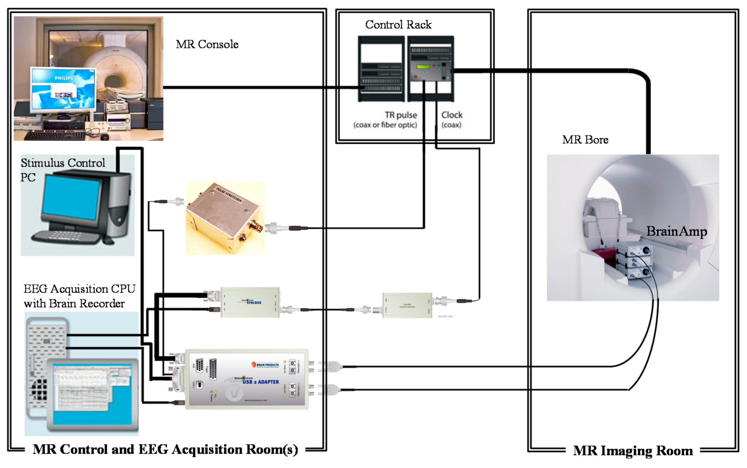
In this study, an EEG cap of 32 standard Ag/AgCl electrodes from BrainProduct (Munich, Germany) was utilized to record EEG data at 5 kHz sampling rate, and the electrodes were positioned according to the extended international 10–20 system with FCz as a reference electrode. Additionally, an electrode was attached beneath the left eye of the subject for electrooculography (EOG) recording. A BrainAmp MR-plus EEG Amplifier (BrainProducts, Munich, Germany) was placed behind a Philips Achieva 3T MR scanner (Best, The Netherlands) at the Sir Peter Mansfield Magnetic Imaging Centre (SPMIC), University of Nottingham, for acquiring the EEG data while the MR scanner was running, and the data were finally recorded into a personal computer by Vision Recorder (Version 1.10) software (Figure 4).

The EEG and MR scanner clocks were synchronized throughout the experiments to guarantee a reliable sampling of the waveforms [7,21]. An 8-channel radio frequency (RF) head coil was used to acquire the fMRI data. As shown in Figure 5A, the amplifier was placed outside the MR bore to isolate it from the vibrations of the MR scanner. Similarly, the cables were run along the cantilever beam and then were coupled to the EEG cap (Figure 5B). Suspending the cable above the mounting of the scanner bed also minimized the scanner’s vibrations [8].

3.1. Study 1: Orthogonal Gradients

EEG recordings were carried out individually from the spherical phantom, the head-shaped phantom, and six human subjects during the execution of a modified echo-planar imaging (EPI) sequence. The purpose of this work was to investigate how the shape of the phantom affects the magnitude of the GA generated by each of the three orthogonal gradients (AP, RL, and FH). Prior to each slice acquisition, three additional gradient pulses, shown in Figure 6, were applied sequentially along the AP, RL, and FH directions. This study was approved by the local Ethics Committee of the University of Nottingham, and each subject provided written informed consent.

The trapezoidal gradient pulse for 30 ms duration consisted of two 10 ms ramps, during which the gradient was changed at a rate of 2 Tm⁻¹s⁻¹ and was kept constant between the consecutive ramps (Figure 6). Successive gradient pulses had a gap of 20 ms. The modified pulse sequence provided clearly defined intervals during which just a single gradient varied in time, allowing the easy separation of the effects of the three different gradients. In a standard gradient echo (GE) EPI acquisition, time-varying gradients are simultaneously applied along multiple axes at high frequencies, and the typical EEG system’s low-pass filtering significantly attenuates and affects the induced voltages, which in turn makes it difficult to differentiate the voltages produced by individual gradient pulses. This introduces a challenge to compute the outcome of the applied time-varying gradient pulse along one specific direction. Therefore, the EEG data were recorded with a frequency range of 0.016–1000 Hz, which ensured the reliability of the acquisition of the EEG data (assuring a higher bandwidth) during the usage of gradient pulses.

3.2. Study 2: EPI Sequence

In the second study, a standard axial, multi-slice GE EPI sequence (repetition time (TR) = 2 s, echo time (TE) = 40 ms, 84 × 84 matrix, 3 × 3 mm² in-plane resolution, 4 mm slice thickness, flip angle = 85°, fold-over direction = AP, SENSE factor = 2, i.e., a two-fold reduction in the number of lines of k-space acquired) was executed while EEG data were recorded. Twenty equidistant slices were acquired within a 2 s TR period, with a resulting slice acquisition frequency of 10 Hz. This standard GE EPI sequence is popular among researchers for characterizing the GA in combined EEG–fMRI data acquisition. Seventy volumes of EEG data were recorded on the phantoms, and 150 volumes were acquired on the human subjects. In this study, the EEG data were recorded with a typical bandwidth (0.016–250 Hz) conventionally used in combined EEG–fMRI studies to keep the EEG signal amplitude in the dynamic range of the EEG amplifier.

EEG data were recorded using the spherical and head-shaped phantoms for six trials in a single recording session and six human subjects in different sessions.

Table 1. Characteristics of the six human subjects tested in the study.

Subjects	Age	Sex	Height (cm)	Weight (lb)
Sub1	29	M	177	160
Sub2	24	F	160	140
Sub3	31	M	180	150
Sub4	35	M	165	154
Sub5	22	F	180	135
Sub6	25	F	158	120

shows the main characteristics of the human test subjects. The subjects were asked to stay as stable as possible to avoid any motion artefacts in the EEG data. Subjects’ EEG data were visually inspected during the EEG recording, and any particular dataset was discarded and re-recorded if any noticeable motion artefacts were observed. In each session, the subjects were placed in the same axial position (+4 cm axial [8]) inside the MRI scanner to avoid any variation due to subject positioning. However, there was some obvious variation due to the head shape and orientation. In the case of the phantoms, in each trial, the phantom was taken out of the scanner and then replaced inside it to mimic the possible variation experienced with the subjects in different recording sessions.

4. Analysis

Brain Vision Analyzer 2 (Version 2.0.1.3417) from BrainProducts and MATLAB (The MathWorks, Natick, MA, USA) were used to analyze the EEG data. Each gradient pulse in the customized EPI sequence commenced with a 10ms period during which the gradient ramped up linearly to a value of 20 mT m⁻¹ giving a rate of change of gradient, dG/dt, of 2 Tm⁻¹s⁻¹. This was followed 10 ms later by a 10 ms period during which the gradient ramped down to zero with dG/dt = −2 Tm⁻¹s⁻¹ (Figure 6). Thus, equal and opposite artefact voltages (in μV) were induced during both periods. The induced GAs were averaged over 30 pulses (Figure 6) to measure the artefact voltage of each electrode, and then we evaluated the average voltage over the central 5 ms of each ramp period, before taking the difference between the positive and negative values. In this way, the effect of any baseline offset and high-frequency fluctuations were eliminated. The severity of the GA depending on the phantom shape was characterized by calculating the root-mean-square (RMS) amplitude of the artefact voltage for each orthogonal gradients across the 31 electrodes (excluding the EOG electrode) located on the phantoms’ or subjects’ head and, finally, by averaging these measures over the phantom trials and human subjects. To graphically depict the difference between the effects of the phantom shape on the GA, spatial voltage maps of average RMS artefact voltages, for each gradient (RL, AP, and FH), were produced using Brain Vision Analyzer 2 for the different phantoms and human subjects. Additionally, the structural similarity (SSIM) was also calculated for the head-shaped phantom and the spherical phantom spatial maps in comparison to the subjects’ spatial maps for each gradient. The SSIM index is a standard method to evaluate the similarity between two images (test and reference images). SSIM assesses [22] the visual impact of three characteristics of an image: luminance I(x,y), contrast c(x,y), and structure s(x,y) with respect to a reference image. The overall index is a multiplicative combination of the three terms:

$$SSIM\left(x,y\right)={\left[I\left(x,y\right)\right]}^{\alpha }·{\left[c\left(x,y\right)\right]}^{\delta }·{\left[s\left(x,y\right)\right]}^{\gamma }$$

(5)

where α, δ, and γ are exponents with the value of 1. I(x,y), c(x,y), and s(x,y) are calculated from the local means, standard deviations, and cross-covariance for images x, y. In this work, the SSIM index was computed to quantify how close or different the spatial maps are.

The EEG artefact waveform of each channel in the study 2 was acquired for a 100 ms (slice) duration. Each waveform was baseline-corrected by subtracting the average channel artefact voltage in the corresponding slice duration. The baseline-corrected voltages were averaged over the slices while excluding the periods of the EEG signal with unacceptable head movements for the subject data. To assess the effect of the phantom shape on the induced GA, the RMS over the slice acquisition period was then calculated for the average artefact on each lead. The average and standard deviation of the EEG data over phantom trials and subjects were also calculated. A paired t-test was applied to the phantoms’ and subjects’ data to assess if there were significant differences between the GAs, which were induced by the EPI sequence due to the variation of the geometric shapes.

The MR data were realigned by using SPM8 [23] to check the head movement, so to keep them stable during the repeated MRI acquisitions. The RMS of the mean corrected realignment parameters (pitch, yaw, and roll, and x, y, and z translation) were calculated for each dataset, and then the average and standard deviation of the phantom and subject trails were computed.

5. Results and Discussion

To demonstrate how the phantom shape in concurrent EEG–fMRI recording affected the induced GA that confounded the EEG data inside the MR scanner, the average contribution of the RMS voltage for each orthogonal gradients was mapped to a 2D spatial voltage representation, as shown in Figure 7. The potential map of the RL gradient of the spherical phantom showed that the frontal, fronto-central, and temporal lobe electrodes contributed to the largest negative voltages, whereas the occipital and parietal lobe electrodes contributed to the largest positive voltages, respectively. However, the potential maps of the RL gradient of the head-shaped phantom and subjects were significantly different from the spherical phantom’s fronto-parietal and parietal lobe electrodes data. In the case of the AP gradient, which is one of the largest artefact-contributing gradient, as shown in previous work by one of this study’s authors [15], the largest positive and negative voltages were recorded in the right and left side of the head-shaped phantom and human subjects. However, the left temporal and parietal lobes of the spherical phantom showed the largest negative voltage contribution. In the FH gradient, there were significant variations reported in previous works [15,19,24] due to the variation of the subjects’ head positions and shapes in the MR scanner bore. In addition, the patterns of the potential maps (induced voltage distribution) of the FH gradient for the head-shaped phantom and human subjects were similar, whereas the map for the spherical phantom was significantly different (Figure 7).

Although it was observed that the head-shaped phantom’s spatial map was very similar to that of the subjects for each orthogonal gradient, it was necessary to quantify this similarity using a mathematical method. The SSIM variation is shown in Figure 8 for each gradient to the compare head-shaped phantom with the spherical phantom in reference to the human subjects. The SSIM was significantly higher (average value, 0.85) for the head-shaped phantom in comparison to the spherical phantom (average value, 0.68) (Figure 8). Interestingly, it was observed that the difference of potential map between the head-shaped phantom and the spherical phantom for the FH gradient was significantly high (Figure 7), but the SSIM value did not reflect this difference. This was due to the variations in the range of the potential for the spherical phantom (i.e., there were several electrodes that contributed to high positive and negative potentials); however, this did not occur for most of the electrodes. It is also important to note that the observed variations of the SSIM values reflected by the error bar in Figure 8, show that the SSIM values varied more significantly for the spherical phantom than for the head-shaped phantom.

To clarify the observed differences in AP and RL in the subjects’ data (as shown in Figure 7), we considered the average RMS voltage for each channel, for the AP gradient (the most contributing gradient), for the subject, the head-shaped phantom, and the spherical phantom (Figure 9). In Figure 9, the means RMS of the induced voltage for the subject data appear highly correlated to the head-shaped phantom data, although the standard deviations for subjects’ data re significantly higher than those of the head-shaped phantom data. This could be explained easily by considering the pulse artefacts and small involuntary movements of subjects’ head during data acquisition, in addition to the brain signal.

Moreover, in the different sessions, even though the subjects were set in the +4 cm axial position inside the scanner, the shape and orientation of the heads did not match completely, which, we believe, greatly contributed to the variation of the standard deviations. To mimic the variation of the orientations of human’s head in different sessions, we took the head-shaped phantom out of the scanner bore and returned it to its position (+4 cm axial position) in different trials, thus slightly altering its orientation. Even though the shape of the phantom remained the same, and no PA and MA occurred in the head-shaped phantom, the observed standard deviation in the head-shaped phantom was due to the altered orientation in different trials. However, Figure 9 shows that the patterns of the potential distribution across different channels for the AP gradients were significantly different for the spherical phantom in comparison to the human head. This clearly revealed that any characterization study of GA to reduce these artefacts in EEG data in concurrent EEG–fMRI experiments might not be accurate when the spherical phantom is used.

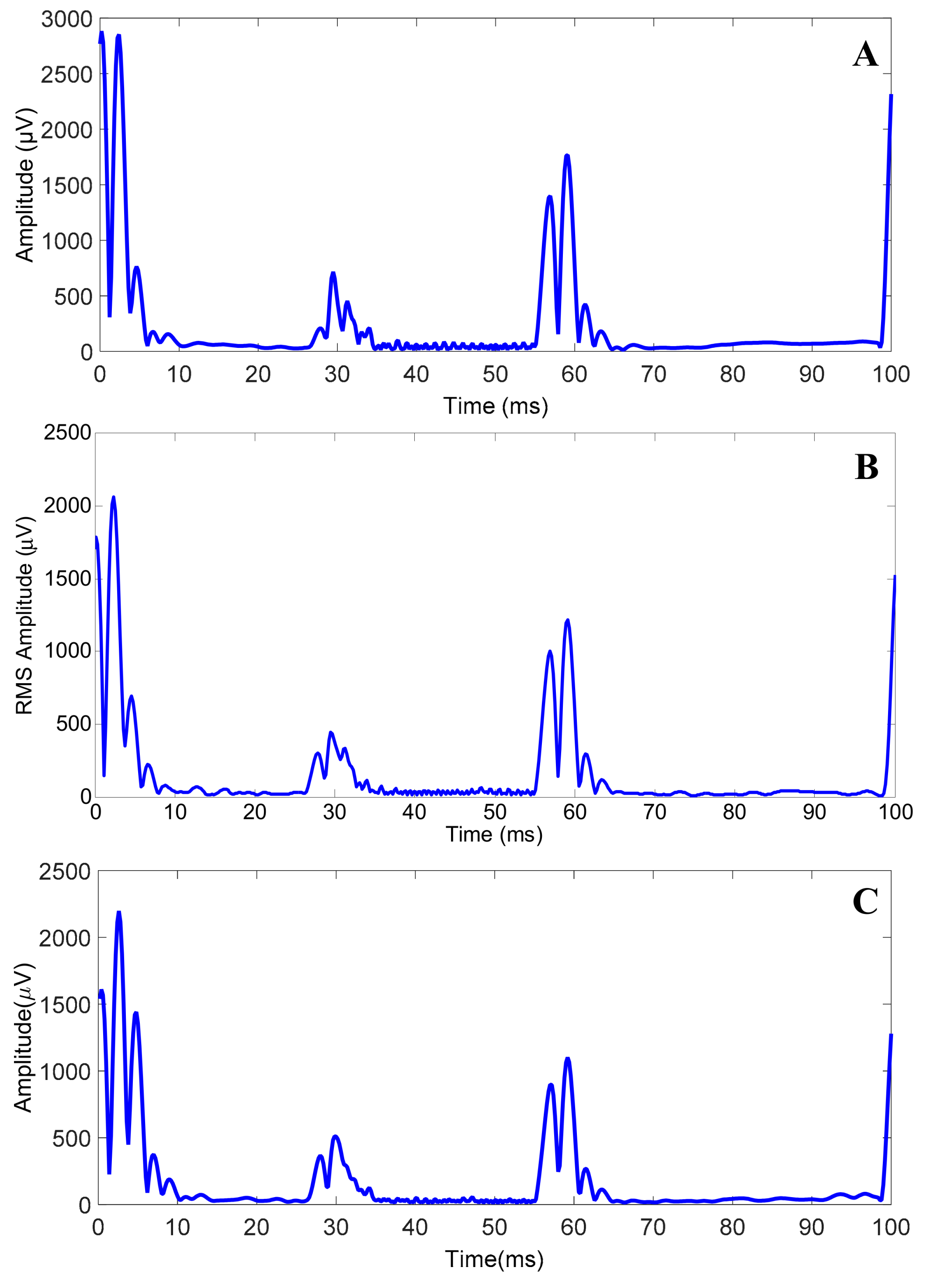
In the study 2, the induced voltages for different trials (subjects and phantoms) were not significantly different. Moreover, the average RMS of the EEG data over time over the channels were 455 ± 21 μV, 368 ± 13 μV, and 383 ± 16 μV for subjects, head-shaped phantom, and spherical phantom trials, respectively. It is clear from Figure 10 that the highest gradient peaks occurred for the same gradients in the human subjects’ and head-shaped phantoms’ data, whereas some variations were observed in the beginning of the R period (fat suppression and slice select). However, the mean RMS value and standard deviation for the human subjects were much higher than those of the phantoms, which also agrees with the findings, as shown in Figure 7 and Figure 9. It can be noted that a higher variation of the standard deviation for the human subjects can be expected, due to the variations of the size and shape of the human head. Moreover, it is evident from the average potential map of the FH gradient for the human subjects (Figure 7) that it is quite different from that of the phantoms, possibly in relation to the shape of the human subjects and of their head. The paired t-test to compare the different trials with the phantoms with the sessions with the subjects showed that the head-shaped phantom and spherical phantom data were significantly different (p < 0.005) from the subjects’ data, whereas the difference between the head-shaped phantom’s and spherical phantom’s data was not significant (p = 0.07).

Furthermore, the movement parameters were identified in the different experimental sessions for all subjects, and no significant deviation among the parameters was observed. The maximum average displacements were smaller than a 0.5 mm translation (z-translation) and a 0.005 rotation (pitch) for all subjects. These movements were small, which implies that the related MA could not be the reason of the similarity of the subjects’ data with the head-shaped phantom’s data. Moreover, the consistency of the RMS amplitude of the induced voltage in time over the channels (small standard deviation) also indicates that this might not be due to MA but, rather, could be the result of the induced voltage.

6. Conclusions

In this study, we investigated experimental EEG data obtained from the simultaneous EEG–fMRI recording of six human subjects and six trials using ahead-shaped phantom, and a spherical phantom in order to study the effects of the phantom shape on the induced GA voltages in the EEG data inside the MR scanner. All the conducted experiments had the same settings and configurations in terms of EEG cap, wiring, and MR scanner. The only uncontrolled difference among the different experiments were caused by the marginal placement shifts of the phantoms in different trials or of the subjects in different sessions inside the MR scanner along with the variations of the orientations. It was found that the head-shaped phantom well mimicked the effects of the GA induced in EEG data by the human head in comparison to the spherical phantom. The SSIM values also supported similar findings. The mean RMS amplitudes of GA in time over the channels for the head-shaped phantom and the spherical phantom were significantly different from that of the subjects, but the difference between the phantoms was not significant. This implies that, even though both phantom shapes mimicked the human head for the overall GA characteristics, the head-shaped phantom reliably mimicked the spatial characteristics of the GA induced by the human head. Therefore, this study recommends the use of a head-shaped phantom instead of a spherical phantom in the future to investigate new cap and wiring configuration designs in order to reduce the induced GA in EEG data derived from the MR scanner.