Large Scale Community Detection Using a Small World Model

Abstract

In a social network, small or large communities within the network play a major role in deciding the functionalities of the network. Despite of diverse definitions, communities in the network may be defined as the group of nodes that are more densely connected as compared to nodes outside the group. Revealing such hidden communities is one of the challenging research problems. A real world social network follows small world phenomena, which indicates that any two social entities can be reachable in a small number of steps. In this paper, nodes are mapped into communities based on the random walk in the network. However, uncovering communities in large-scale networks is a challenging task due to its unprecedented growth in the size of social networks. A good number of community detection algorithms based on random walk exist in literature. In addition, when large-scale social networks are being considered, these algorithms are observed to take considerably longer time. In this work, with an objective to improve the efficiency of algorithms, parallel programming framework like Map-Reduce has been considered for uncovering the hidden communities in social network. The proposed approach has been compared with some standard existing community detection algorithms for both synthetic and real-world datasets in order to examine its performance, and it is observed that the proposed algorithm is more efficient than the existing ones.

1. Introduction

In a real world, various categories of networks play different roles in the society for different purposes viz. social networks, which represents social interactions among human beings in society, citation networks that represent the articles of various authors published in the particular field and their associated citations in other papers, technological networks that represent the distribution of resources, biological networks that represent protein–protein interaction in the network, etc. Social networks are considered as having interesting research domains due to their characteristics of involving human social activities. Network evolution [1], network modeling [2], centrality analysis [3], information diffusion [4], link prediction [5], and community detection [6] are some of the interesting research directions in social networks. Power-law degree distributions [7], small world networks [8], and community structures are some of the important properties observed in the social network.

Communities are found to be one of the most important features of large-scale social networks. Uncovering such hidden features enables the analysts to explore the functionalities in the social network. There exists quite a good number of definitions of community depending on the contexts pertaining to different applications. However, as per few number of commonly accepted definitions, they are considered to be a group of nodes that have a dense connection among themselves as compared to sparsity outside the group. Communities in the social network represent a group of people who share common ideas and knowledge in the network. Hidden communities can be explored through learning from social dynamics in the network [9]. Their identification helps in getting insight into social and functional behavior in the social network. However, due to unprecedented growth in the size of social networks, it is quite a hard task to discover subgroups in the network within a specified time limit. Real-world social networks are observed to follow the power-law in both degree-distribution and community size distribution [7].

A distributed framework like Hadoop may be considered as a better alternative for processing a large volume of data in complex and heterogeneous social networks. Hadoop internally uses a Map-Reduce algorithm for processing computation in multiple nodes in a cluster. It uses a dedicated file system known as Hadoop Distributed File System (HDFS) for storing data across multiple nodes in the cluster. A network is said to have small-world properties if the geodesic distance between any two nodes is small. In a small world network, for a fixed average degree, the average path length between pairs of the node in the network increases logarithmically with the increase in number of nodes or, in other words, small world network exhibits pure exponential growth with respect to walk-length in the network [10]. These inherent properties of real-world networks make it difficult for graph mining. There exist a plethora of community detection algorithms in the literature, where most of them emphasize maximizing the quality parameter in order to detect communities in a large-scale network. Sometimes, they are insignificant in exploring communities in a reasonable amount of time, due to the resolution limit of modularity [11]. The community detection algorithm is said to be faster and efficient, only if it follows a small world network phenomenon. The small world network concept is based on the six degrees of separation principle [12].

In this study, the Map-Reduce approach has been used to uncover the hidden communities in a large-scale network. Map-Reduce algorithms always follow two crucial phases: one is mapper and another one is the reducer. In this work, mapper phase has been used in mapping the nodes to their corresponding communities. An effort has been made to discover the communities using a small world model. In reducer phase, nodes are being clustered based on their walk length and similarity index ($\eta$) with the source node. Random walk based similarity index is introduced to measure the strength of social ties.

The subsequent sections of this paper is organized as follows: in Section 3, some preliminaries about community structure, small world network, power-law degree distribution and clustering coefficient has been discussed. Section 4 presented the random walk process in the network. In this section, a new similarity index has been devised based on a random walk in the network. The proposed methodology has been presented in Section 5. Community detection and clustering phase have been discussed in this section. Section 6 presented the implementation part of the work. Experimental results have been discussed in Section 7. Section 8 presents the possible threat to validation of the work. Conclusions and future work have been discussed in Section 9.

2. Related Work

Community detection is similar to a graph partitioning problem. Most of the graph partition methods are based on optimizing a quality function. Girvan and Newman have proposed the first community detection algorithm, which is based on a hierarchical partitioning problem in a graph. In their work, modularity has been chosen as the objective function for accessing the quality of obtained partition [13]. In this algorithm, edges are removed iteratively in the order of their edge-betweenness value until it reaches the maximum modularity. Edge-betweenness value of an edge can be expressed as the number of shortest paths between a pair of nodes that passes through the edge. Modularity taken in this paper does not consider the information about unrelated pairs inside the network. A new modularity known as MIN-MAX modularity has been devised by R. Behera and M. Jena to optimize the community partitions in the paper [14]. It not only considers dense connections within the group, but it also gives the penalty to unrelated pairs within the group.

Random graph is a kind of graph where edges are distributed randomly among the nodes, but, unfortunately, it does not resemble a real-world network. A random graph generation model was proposed by Watts and Stogatz, which helps in generating the random graph with small world properties like average short path length and high clustering coefficient [15]. It has been observed that a small world network lies in between regular and random graphs. Communities are frequently observed in small world networks.

Ego network is the group of nodes consisting of a central actor and other nodes that are directly connected to it. They resemble with the properties of the small-world network. The central node in the ego network may have highest influential ability as compared to other nodes in the network. Exploring focal nodes may helps in modeling influence propagation in the network [16]. The social network allows users to make a group based on the common interest or common event happening in their social life. However, automatically, group construction is a difficult task when friends are added or removed dynamically in their social life. Authors McAuley and Leskovec have proposed an efficient model that enables detecting ego circles in large-scale networks that capture both structural and user profile information [17]. In this paper, the author has developed a model where a user can belong to different ego circles. This model allows the user to detect an overlapping community as well as hierarchically nested circles in a large-scale social network. Social circles in ego networks have a great impact on the evolution of the network.

Three fundamental network models come into the picture while discussing structural parameters of the network. The first one is the random network where nodes and edge distribution is random over the network. Degree distribution in the network follows binomial or Poisson distribution in a random network [18]. It is similar to the homogeneous network where most of the vertices are having the same degree. The small world model is another kind of network model that lies in between random and lattice network models. It exhibits a high clustering coefficient like a lattice network and smaller average path length like the random network. Degree distribution of a small world network follows the binomial distribution. A real-world network follows the power-law degree distribution that resembles the scale-free network model. A small world network model may have the scale-free distribution like a real-world social network. Chopade and Zhan have discussed the structural and functional characteristics for community detection process in the complex social network in their paper [19]. Community detection based on the structural parameter of the network topology has attracted an interest of research as compared to community detection based on the functional parameter of the network.

Several methods for community detection techniques have been developed and each has its own strength and weakness [6,13,20,21]. An efficient community detection method that considers both local and global information about topological structure has been explained by De Meo et al. [22]. Global information about the network topology helps to yield good results about community; however, it is not suitable for the large-scale complex network. Large scale network needs to be preprocessed through dimension scaling in order to map the global information to local one [23]. Local information about network topology may lead to faster community detection but are less accurate in nature. In this paper, the community detection process is based on optimizing the modularity value based on global information about the structure and yet is able to compare scalability of the network with local methods. In this work, communities have been detected in two phases. In the first phase, walk length for each node from a source node has been detected using an information propagation model, which is based on the random walk in the network. In the second phase, Euclidean distance between the nodes has been used for clustering process to partition the network.

Steve Gregory proposed label propagation algorithm for community detection in linear time complexity [24]. The main idea behind the algorithm is that a node is more likely be a part of that community, to which its maximum neighboring nodes belong. Labeling of a node is propagated through its neighboring nodes in multiple iterations until a label is confined to a group of nodes. It is the fastest available community detection method, which has been claimed to have linear time complexity. The community detection algorithm spends most of the time measuring the similarity values between a pair of nodes, especially in the case of unweighted graphs.

Community detection using random walk has been discussed by Pons et al. [25]. The algorithm discussed in this paper is well known as the Walktrap algorithm. The intuition behind the Walktrap algorithm is that a walker more likely gets trapped inside the dense region if it moves randomly inside the network. In this paper, the author has made an effort in discovering clusters by observing the movement of the walker inside the network. The time complexity of Walktrap algorithm is found to be $O\left(m{n}^2\right)$ in the worst case, where m is the number of edges and n is the number of nodes in the network. In this work, similarity between nodes has been calculated based on the random walk in the network.

Spin-Glass is a unique community detection algorithm that is based on the statistical mechanics of spin around the network [26]. The expected number of communities has been overestimated in the community detection and It has the worse approximation for the community when complexity and size of the network increases. However, it works fine for a small world model but too much expensive. Similarity between objects is determined by the spin associated with objects in graph configuration. Similarity between nodes is higher if their spins are of the same order. Communities are detected based on Pott’s spin-glass model.

In the literature, most of the community detection algorithms deal with the undirected network. However, the real-world complex network often resembles the directed graph. Agreste et al. have made an extensive comparison of community detection algorithms for the directed network [27]. Infomap and Label propagation algorithms are the first ones to implement in the directed network. However, for the sake of simplicity, we have implemented these two algorithms on the undirected network. Peng and Lill have proposed a framework for mapping the community detection algorithm from undirected to the directed network. They have applied modularity optimization technique for obtaining optimal partitioning of the network [28].

Xiaolong et  al. have proposed an optimized community detection algorithm, which is based on the vector influence clustering coefficient and directed information transfer gain of vertices in the network. They have implemented their algorithm on the directed network. In their work, they have also proposed an efficient optimization parameter (target optimal function) to evaluate the community partition in the network [29].

Rosvall and Bergstrom have developed an elegant community detection algorithm for discovering modules in a large-scale network, which is known as Infomap [30]. It is based on an optimizing a map function. This algorithm is similar to the Louvain algorithm, where, initially, each node in the network is assigned to a module, and, in each iteration, nodes in the modules are migrated themselves into the nearest module in order to minimize the map function. The proposed algorithm is quite similar to this algorithm where nodes are migrated into the modules based on the detected walk length in which nodes are discovered. Nodes belong to the same module are forced to migrate into another module to optimize the map function at the time of rebuilding the network structure. As a result, nodes assigned to one module at one point may differ from the assigned module at a later point in time. The Infomap algorithm is well suited for a small network. Its accuracy is found to be best as compared to other standard community detection algorithms [31].

Since the real world network follows the power-law degree distribution and quite complex in nature, traditional algorithms are practically inefficient unless it is implemented in some parallel architecture. The proposed work is similar to random walk community detection algorithm proposed by Pons et al. [25]. However, we have considered the concept of a small world model to evaluate the similarity between vertices in the network. Unlike the Walktrap algorithm, which processes the whole network for quantifying the similarity between the vertices, the proposed similarity measure has been calculated in less number of steps in a recursive manner that improves the performance of community detection. The proposed algorithm is further improved by implementing it in a Hadoop distributed platform. The proposed algorithm may surpass previously discussed community detection algorithms in terms of accuracy, as most of them are based on either a regular graph model or a random graph model [15]. Both of these models have less resemblance with the real-world network. However, a small world model closely resembles the real-world network.

The proposed algorithm behaves in a more consistent manner as compared to Infomap and the Spin-Glass community detection algorithm. The Infomap algorithm is based on the information flow in the network, which is calculated through random walk probability in the network. Huffman coding is used to generate the two-level encoding schema for the network. Community partitioning is identified by optimizing the mapping function that tries to compress the encoded schema by simulated annealing. This approach seems to be unrealistic and inconsistent for a large-scale network. The optimizing criteria in the Spin-Glass algorithm are similar to the Infomap algorithm. The proposed algorithm outperforms these two algorithms due to its efficient optimizing criteria for community evaluation.

3. Preliminaries

3.1. Structural Definition of Community

Social network may be represented in the form of a graph $G=(V,E)$, where V is the set of nodes and E is the set of edges in graph G. A group of nodes c∈V is said to form a community if it satisfies the following condition:

$$\frac{2e_{in}}{n_c(n_c-1)}>\frac{2E}{V(V-1)}>\frac{e_{out}}{n_c(V-n_c)},$$

(1)

where $e_{in}$, $e_{out}$ are the number of edges existing inside the community and number of edges existing from a node in the community to a node outside the community respectively. $n_c$ is the number of nodes within the community c. First and third part of Equation (2) corresponds to the fraction of number of links within the communities and between the communities in the graph, respectively. The middle part corresponds to the density of the graph. For a graph with community structure, a fraction of intra-community links are expected to be larger than graph density and graph density is expected to be larger than a fraction of inter-community links in the graph.

3.2. Small World Phenomenon

Small world phenomenon is one of the inherent principles behind the analysis of today’s large-scale social network, which indicates that any two people in the network can be linked by a small number of acquaintances [10]. It may be observed that there always exists a path of short length that can be discovered using local information. A small world network is often associated with a high clustering coefficient and its characteristic path length decreases more rapidly than the clustering coefficient as the randomness increases.

Definition 1. 

A graph is said to be a small world network if average path length $L_{avg}$ is less than or equal to the path length $L_{rand}$ and average clustering coefficient $C_{avg}$ is strictly less than clustering coefficient $C_{rand}$ in a random degree distribution of the graph:

$$L_{avg}⪯L_{rand}and{C}_{avg}\prec C_{rand}.$$

(2)

This phenomenon is based on the six degrees of separation principle.

Definition 2. 

Six degrees of separation is the principle, which indicates that every two people in the world is connected with a chain of no more than six acquaintances.

Small world network exhibits the following important characteristics:

• Short Average Path Length;
• High Clustering Coefficient;
• Exhaustive search using local information.

3.3. Power Law Degree Distribution

The degree of a user in a social network is the number of relationships that the user maintains. Distribution of relationships among users is known as degree distribution. A network is said to be scale-free if it follows power-law degree distribution [12].

Definition 3. 

A network is said to have power-law degree distribution if a fraction of nodes having degree k in the network depends on the power of k with some constant. Social network often follows power-law degree distribution as indicated by the following equation:

$$p_d=k{d}^{-\gamma },2\le \gamma \le 3,$$

(3)

where $p_d$ is the fraction of nodes having degree d, k and γ are power-law intercept and power-law exponent, respectively. Usually, γ ranges from 2 to 3.

3.4. Clustering Coefficient

Clustering coefficient is a measure used to define the network as the small world network. Clustering coefficient defines the friendship transitivity in a network [32]. This measure can have two versions: one is local and another one is global. Local clustering coefficient is associated with each node in the network where global clustering coefficient represents the clustering density for the whole network.

3.4.1. Global Clustering Coefficient (GCC)

Small world network is often observed to have high global clustering coefficient. GCC of the network is defined as the ratio of a number of triangles and the possible number of connected triplets in the network. A triplet is the set of three connected nodes in the network. Each triangle in a network contributes to three triplets. GCC of a network may be framed as below:

$$GCC=\frac{3\times Numberoftriangleinthenetwork}{Numberoftripletsinthenetwork}.$$

(4)

3.4.2. Local Clustering Coefficient (LCC)

LCC signifies the tendency of a node to form a cluster. The higher the clustering coefficient of a node, the more chances to be involved in a cluster. It is defined as the fraction of edges existing between the neighboring nodes to the total number of edges possible. LCC for a node i can mathematically be represented as follows:

$$LC{C}_i=\frac{2\left|(u,v):(u,v)\in Eandu,v\in Neighbor\left(i\right)\right|}{n_i(n_i-1)}.$$

(5)

Here, $(u,v)$ is the edge between neighboring nodes, E is the set of edges in the network, Neighbor $\left(i\right)$ is the set of neighboring nodes of i and $n_i$ is the number of elements in the set. The average of local clustering coefficients for all of the nodes may be considered as the global clustering coefficient.

4. Random Walk

Community detection in a large complex network can be carried out by capturing the topological structure using random walk in the network. The intuition behind random walk is that the network tends to be trapped inside a denser region (community) for a longer period of time. This idea can be used for inclusion of nodes in the community. In this paper, an efficient similarity metric based on the random walk has been proposed to include a node in the community. This metric may provide the following features:

• Structure of the network is well captured in the process of community detection;
• It can be used in an agglomerative hierarchal clustering;
• Computation to find community may be more efficient.

Social network can be represented in the form of a graph, where nodes represent social entities and edges represent relationships between the entities. The graph can be stored in the form of adjacency matrix A, where $A_{ij}=1$, if there is an edge, existing between nodes i and j, and 0 otherwise.

Random walk in a graph is the process of visiting a neighboring node randomly from the source node and continuing the process of visiting throughout the graph. Random walk process is well explained on the basis of Markov chain in which each node corresponds to vertices in the visited path [33]. In this paper, transition matrix obtained by Random walk in the graph has been considered for detection of communities. Transition matrix describes the probability of visiting each node from every other node in k number of steps i.e., $T_{i,j}^k$ corresponds to the probability of visiting node j from i in k number of steps. $T^1$, $T^2$, $T^3$ and $T^k$ are the transition matrices for random walk corresponding to 1, 2, 3 and k walk length, respectively. Transition probability from vertex i to vertex j in one length random walk is defined by the following equation:

$$T_{ij}^1=\frac{A_{ij}}{d_i},$$

(6)

where $A_{ij}$ is the adjacency matrix of the network and $d_i$ is the degree of vertex i.

Property 1. 

Probability for a random walker to visit a node j from node i in walk length that tends to infinity depends only on the degree of j, rather than degree of the source or the intermediate node. It may be represented as:

$$\underset{k\to \infty }{lim}{T}_{i,j}^k=\frac{d_j}{2E},$$

(7)

where $d_i$ is the degree of i and E is the total number of edges in the network.

Property 2. 

Ratio of probabilities for a random walker that visits a node from i to j and j to i through a fixed walk length depends only on the degree of i and j. It may be represented as follows:

$$\frac{T_{i,j}^k}{T_{j,i}^k}=\frac{d_j}{d_i}.$$

(8)

Vertex Similarity Based on Random Walk

Vertices belonging to the same community seems to have similar behavior as compared to vertices outside the communities. Any two nodes inside a community look the same way as other nodes in the network. We may consider an example of a random walk of length k in graph $G(V,E)$, which represents a social network. The probability of visiting all nodes from all other nodes in the network through k length random walk is represented by transition matrix $T^k$. Each tuple in the transition matrix corresponds to probabilities of visiting all other nodes from node i in k walk length. These probabilities are based on structural information in the network. From the structure of the network, the following inferences may be drawn:

• If two nodes i and j, are in the same community, the probability of visiting node j from i would be higher as compared to visiting a node outside the community. In addition, converse may not be true i.e., if the probability is high, it does not mean that they belong to the same community.
• The probability $T_{i,j}^k$ depends on the degree of j because the walker tends to visit towards vertices, where the degree is high.
• Two vertices belonging to the same community tend to see all other vertices in the same way:

  $$\mathrm{i}.\mathrm{e}.,T_{i,m}^k\approx T_{j,m}^k,\forall i,j\in \mathrm{same}\mathrm{community}\mathrm{and}m\in [1,n].$$

  (9)

In this paper, similarity between two vertices are identified from the transition matrix $T_{i,j}^k$ based on the walk length k. Probability of reaching one node from another would be different for different walk lengths. Similarity between i and j for k walk length can be computed by the Euclidean distance between row vectors corresponding to nodes i and j, in matrix $T^k$:

$$Sim(i,j)=\sqrt{\sum _{l=i}^n\frac{{(T_{i,l}^k-T_{j,l}^k)}^2}{d_l}},$$

(10)

where $d_l$ is the degree of vertex 1.

5. Proposed Methodology

Detecting communities in a social network having a good number of nodes in a reasonable amount of time is a challenging task due to its size and structure. In this work, distributing computing environment has been considered for processing large-scale networks. Hadoop is a framework applied to solving the complex problem by distributing the computation in multiple nodes in the cluster. Hadoop implicitly schedules the pieces of task on the different computing node. It automatically takes care of load balancing and resource scheduling over the cluster of nodes. Users need not worry about the internal execution policy. However, users can provide the application specific mapper and reducer program to the Hadoop framework. Users have the control over the Map-Reduce program structure but does not have control over execution environment. In this work, the community detection process in Hadoop has been carried out in the following two phases:

• mapper phase,
• reducer phase.

Prior to the computation in Hadoop, the random walk process has been carried out in order to visit all the nodes in the network. In this work, similarity values between all pair of nodes have first been calculated from the transition probability matrix. Transition matrix has been generated separately for random walk lengths 1 to 3.

In the mapper phase, community memberships of nodes are being evaluated by using the local information available at each node. In a Small world network model, quick navigation is possible through two fundamental processes: one is to find the short chain of acquittance and the other is to use only local information regarding structure around the node. The community detection process starts from a randomly selected source node. Neighboring nodes who have similarity value less than the threshold value, $\eta$, are identified and then included in the same community, to which the source node belongs. Here, $\eta$ is treated as the clustering parameter for a small world model that determines the probability of having a connection between two nodes in the network. Small world model parameters have been determined based on the random walk in the network. Once a node has been mapped with a community number, the node is temporarily deleted from the graph in order to reduce the computation. For the sake of simplicity, the undirected graph has been taken into consideration. It is observed that a real world social network follows a small world network, or, in other words, by following a small number of steps, one can visit all other nodes in the network. Mapper phase nodes are mapped into their community in the order of their reachability from the source node. Steps adopted in the mapper phase are shown in Algorithm 1. The execution flow for community detection is presented in Figure 1.

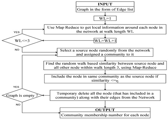
Figure 1. Execution flow for community detection using small world phenomenon.

Algorithm 1: Community detection using small world phenomenon (CDSW).

Mapper (Source Node, Community Membership, Graph G)

Input  : The social network graph in the form of edge lists.

Output  : Community Membership for each node in the form of (Key,Value) pair.

Here Community Membership is the Key and (Walk Length (WL), Node ID) is the Value.

Initialization  :

Select a node randomly as the Source Node.

C.append (Source Node)

$C^{{}^{\prime }}$ = NULL

WL=0, Community Membership=1

Emit(Community Membership, $WL$, Source Node, NULL)

1. for $WL$=1 to 3

2.      for all v in C

3.          for each neighbor ∉$C^{{}^{\prime }}$ and Sim(Node v, Neighbor Node) ≤    $\eta$

4.             Emit (Community Membership, $WL$, Neighbour Node)

5.          endfor

6.           Delete v from both Graph and C

7.      endfor

8.    C = $C^{{}^{\prime }}$

9.    Delete the nodes in $C^{{}^{\prime }}$, because they are already visited.

10. end for

11. Community Membership++

12. Source Node = Random source node for next community

13. if graph is empty

14.           exit()

15. else

16.           Mapper(Source Node, Community Membership, Graph)

17. endif

In the reducer phase, the clustering process is being carried out by developing a dendrogram structure for the network. Dendogram structure is the hierarchical structure from where one can identify communities at a certain level of granularity. If the structure is partitioned at a certain level, the groups formed below the partition can be considered as individual communities. The input to the reducer phase is in the form of the key–value pair where community number detected in a mapper phase is treated as the key and the rest of the parameters such as walk length, node id, and a number of detected community together is treated as the value for the corresponding key. Dendogram structure is detected at two levels. One is at the inner level of each community and the other at a global level where each detected community is treated as a node structure. At the inner hierarchy, all of the nodes are detected in the same walk length in mapper phase belong to the same level in the dendrogram structure. Nodes that are assigned in the same community at a particular walk length are grouped into a community. To develop the dendogram structure at higher level hierarchy, we have proposed an efficient distance measure between each pair of communities that depend on the dissimilarity between the communities. It is calculated by measuring maximum dissimilarity that may be possible between any two nodes of different communities. It can be mathematically represented as follows:

$$distance(C_i,C_j)=max\left\{sim(i,j)\right\}textwhere\forall i\in C_i,\forall j\in C_{j}andi\ne j,$$

(11)

where $C_i$ and $C_j$ are the two different communities and i and j are the two nodes belonging to $C_i$ and $C_j$, respectively. Here, $sim(i,j)$ has been already calculated from Equation (10). The pair of communities is first identified with minimum distance for grouping at the same level in the dendogram structure. After the grouping, it is treated as a single community. The next pair of communities is then identified by following the same procedure. The process is continued until all of the same communities are involved in the structure. The steps followed for obtaining the dendogram structure is presented in Algorithm 2. The clustering process of detected communities is presented in Figure 2.

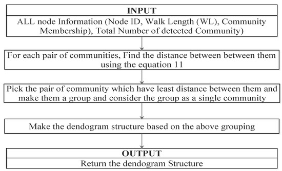
Figure 2. The process of developing dendogram structure to identify communities.

Algorithm 2: Clustering of detected communities.

Reducer(Community_Number, Walk_Length, Node_Id, Parent_Id)

Input  : Community ids for each node in the form of (Key,Value) pair.

Here Community_Number is the Key and (WL, Node_Id, Parent_Node) is the Value.

Output  : Community Structure in the form of Dendrogram.

1. for every Community_Number sort Node_Id according to their Walk_Length

2.     for every Walk_Length in Community_Number

3.               Combine the nodes at the same level

4.                Increase the level for the next walk_Length

5.     end for

6.     Choose the next Community for further clustering

5. end for

2. for every pair of communities

3.               Find the distance by using Equation (11).

3.               Combine the communities with smallest distance at the same level

4.                Increase the level to choose next pair of communities

5. end for

6.

5. Return the Dendrogram structure for the Network.

6. Implementation

6.1. Metrics for Evaluation Performance

The following evaluation metrics have been considered for measuring performance of the proposed algorithm.

• Normalized Mutual Information ($NMI$): NMI is a suitable measure to compare the quality of different community partitions. It can be evaluated with the help of confusion matrix ($CM$), where each row corresponds to the community, present in the real partition and each column corresponds to the community, detected through the proposed algorithm. Confusion matrix has been obtained based on the number of communities and community memberships for each node, which is available as ground truth in the datasets [34,35]. Each element in the confusion matrix $C{M}_{ij}$ represents the number of vertices in ith real community, which is also present in jth detected community. $NMI$ of the detected partition may be formulated as:

  $$NMI(X,Y)=\frac{-2{\sum }_{i=1}^{n_X}{\sum }_{j=1}^{n_Y}C{M}_{ij}log(\frac{C{M}_{ij}CM}{C{M}_{i}C{M}_j})}{{\sum }_{i=1}^{n_X}C{M}_{i}log(\frac{C{M}_i}{CM})+{\sum }_{j=1}^{n_Y}C{M}_{i}log(\frac{C{M}_j}{CM})},$$

  (12)

  where X and Y are the community partition structure corresponding to ground truth and detected structure, respectively. $C{M}_i$ and $C{M}_j$ indicate the communities in true and detected community partition, respectively.
• Modularity (Q): Modularity is a metric used to quantify the quality of community partition. This measure is proposed by Girvan and Newman [13]. It is defined as the difference between the number of edges existing inside the communities and the number of edges, which would have been present in a random assignment in the network with similar degree distribution. The expected number of edges between i and j with degree $d_i$ and $d_j$, respectively, is $d_i{d}_j/2$. Modularity value for a given partition P = {$c_1,c_2,.....c_k$} in the graph $G=(V,E)$ is defined as follows [36]:

  $$Q=\frac{1}{2E}\sum _{C_l\in P,\left(1\le l\le k\right)}\sum _{i,j\in C_l}\left(A_{ij}-\frac{d_i{d}_j}{2E}\right).$$

  (13)
• F-Measure: F-measure is a metric used to find the accuracy of the proposed algorithm when the ground truth about the communities are available in the dataset. It is the harmonic mean of precision and recall, where precision and recall can be obtained from the confusion matrix obtained from the experiment. Confusion matrix for community detection has been described in Table 1. In this work, all pairs of nodes are considered to get the value of a, b, c and d for each dataset considered, where
  Table 1. Confusion matrix for community detection.

  		Ground Truth
  		$\mathit{C}\mathbf{(}{\mathit{v}}_{\mathit{i}}\mathbf{=}\mathit{C}\mathbf{\left(}{\mathit{v}}_{\mathit{j}}\mathbf{\right)}$	$\mathit{C}\mathbf{\left(}{\mathit{v}}_{\mathit{i}}\mathbf{\right)}\mathbf{\ne }\mathit{C}\mathbf{\left(}{\mathit{v}}_{\mathit{j}}\mathbf{\right)}$
  Clustering result	$C\left(v_i\right)=C\left(v_j\right)$	$a\left(TP\right)$	$b\left(FP\right)$
  	$C\left(v_i\right)\ne C(v_j$	$c\left(FN\right)$	$d\left(TN\right)$

  ‒

  a = number of pairs, in the same community in ground truth and assigned in same community after community detection. It is treated as True Positive ($TP$).

  ‒

  b = number of pairs, belonging in different communities but assigned in same community after community detection. It is treated as False Positive ($FP$).

  ‒

  c = number of pairs, belonging in same communities but assigned in different communities after community detection. It is treated as False Negative ($FN$).

  ‒

  d = number of pairs, belonging to different communities and assigned in different communities after community detection. It is treated as True Negative ($TN$).

  Precision can be defined as follows:

  $$Precision=\frac{TP}{TP+FN}=\frac{a}{a+c}$$

  (14)
  Recall can be defined as follows:

  $$Recall=\frac{TP}{TP+FP}=\frac{a}{a+b}$$

  (15)
  F-measure can be defined as follows:

  $$F-measure=\frac{2\times Precision\times Recall}{Precision+Recall}.$$

  (16)
• Execution Time: A major issue in community detection algorithms is to uncover communities in a reasonable amount of time. In this paper, performance of different algorithms has been measured in terms of execution time. Execution time includes only CPU running time without considering the external time factor. Execution time for all community detection algorithms has been measured in machines with the i7 processor with 3.4 GHz clock speed. Running times have been measured in units of seconds.

6.2. Datasets Used

Social network dataset is often represented in the form of the graph structure, where nodes in the graph represent social entities and edges represent the relationships among the entities. In this paper, the experiment has been carried out using both synthetic and real-world datasets. Details of the datasets are listed in Table 2.

Table 2. Datasets used for evaluation.

Datasets	Nodes	Edges	No. of Communities	Average Path Length	Clustering Coefficient
Synthetic data1	10,000	27,365	620	8.79	0.326
Synthetic data2	20,000	31,569	900	11.59	0.169
com-DBLP	317,080	1,049,866	13,477	7.23	0.6324
com-Amazon	334,863	925,872	75,149	28.67	0.3967
com-Youtube	1,134,890	2,987,624	8385	11.38	0.0808

6.2.1. Synthetic Dataset

The Lancichinetti–Fortunato–Radicchi (LFR) benchmark has been used for generating synthetic data for the social network. This benchmark is observed to be an established one for evaluating different community detection algorithms. Synthetic networks that resemble real-world social networks have been generated by tuning a set of parameters in an LFR benchmark. Parameters in the LFR benchmark include a number of nodes in the network, degree distribution, community size distribution, the maximum and average degree of node, etc. The degree distribution in the network follows the power-law in the LFR benchmark. The probability of having a node with degree k varies with the parameter $\gamma$ as mentioned below:

$$P_k\alpha k^{-\gamma }.$$

(17)

Here, the value of $\gamma$ is assigned to vary between 2 to 3 in order to resemble real-world social networks. $\mu$ is considered as another parameter in the LFR benchmark, which is also known as mixing parameter. A small value of $\mu$ indicates more sparsity between the planted communities in the network. The complexity of the network increases by scaling the $\mu$ value. In this paper, the complexity of the network has been increased by scaling mixing parameter from 0.2 to 0.5. $\beta$ parameter in LFR has been considered for community size distribution in the network. $\beta$ value often varies between 1 and 2. For each of the synthetic datasets, performance of algorithms has been measured by tuning mixing parameter from 0.2 to 0.5 by increasing 0.05 at each step. Thus, a total of fourteen data points have been generated from two artificial datasets listed in Table 2 and performance has been measured for these data points.

6.2.2. Real World Datasets

Real-world datasets are more complex and heterogeneous as compared to synthetic data. Revealing communities in real-world networks is a NP (non-deterministic polynomial)-hard problem. For measuring the performance of the proposed algorithm, the following real-world datasets have been taken into consideration:

• DBLP;
• Amazon;
• Youtube.

All of these datasets have been collected from the Stanford Large Network Dataset Collection (SNAP), which is publicly available for social network analysis [35].

7. Experimental Results

The experiment has been carried out on a cluster of five nodes, each with an i7 processor with 3.4 Ghz clock speed. The master node has a configuration with a 1 TB hard disk and 10 GB RAM. It also acts as a worker node. Each of the other four nodes acts as a slave or worker node. They all have a symmetric configuration with 1TB hard disk and 20 GB of RAM. A similarity measure based on the random walk has been used to identify the neighboring nodes for inclusion in the community. The threshold value for similarity measure has been considered to be 0.5. A number of synthetic datasets have been generated by tuning the parameters available in LFR benchmark. The proposed algorithm i.e., CDSW, has been implemented both on synthetic and real-world social network datasets. It has been compared with the following community detection algorithms, available in literature:

a

Infomap Community Detection (INF) [30];

b

Spin-Glass Community Detection (SG) [26];

c

Girvan Newman Community Detection (GN) [13];

d

Walktrap Community Detection (WT) [25].

NMI is one of the accepted measures for comparing detected clusters with ground truth partitions. NMI for each partition obtained from different algorithms has been evaluated. The higher the NMI value, the better is the community partition. Figure 3a shows the box plot analysis for NMI of all data points. It is observed that the median of NMI for the proposed community detection algorithm using small world phenomenon (CDSW) is more than 0.8, which is better as compared to other algorithms. Minimum NMI for CDSW algorithm is higher than the minimum value for other algorithms. The WT algorithm performs better with respect to NMI, which is close to the performance of the proposed algorithm.

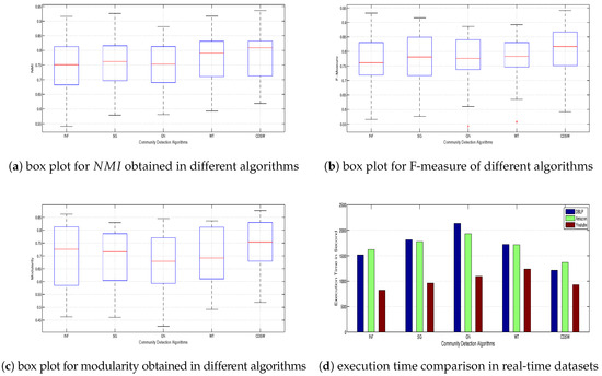
Figure 3. Comparative study of different community detection algorithms.

Figure 3b shows the box plot analysis of F-measure for different algorithms. F-measure is related to the accuracy of algorithms. It has been calculated using the confusion matrix for community partition. The structure of the confusion matrix has been presented in Table 1. From the Figure 3b, it is observed that the median F-measure of the CDSW algorithm is higher than 0.85. Although the maximum of F-measure values for the CDSW algorithm is not as good as those obtained for WT and GN algorithms, its average and maximum values have been observed to be higher than all other algorithms.

Figure 3c shows the box plot analysis of modularity value for community partition generated from different algorithms. The higher the modularity value, the better is the community partition. Modularity value decreases when link density between the communities or the value of mixing parameter $\mu$ increases. Median modularity value for the proposed algorithm is observed to be better as compared to other community detection algorithms. Modularity values obtained from Spin-Glass and Infomap algorithms are relatively similar. From Figure 3c, it is observed that the CDSW algorithm provides better community structure as compared to other traditional algorithms.

In the social network, the number of entities and their relationships are observed to be increasing exponentially. Since community detection in the large-scale network in a reasonable amount of time is the focus of this study, an effort has been made in measuring execution times for different algorithms in community detection. Figure 3d shows the comparative study of execution time for different community detection algorithms. The structure of synthetic network changes when mixing parameters of benchmark increases. In this work, comparative analysis of execution time has been carried out separately for both synthetic and real-world datasets. The comparative analysis of execution time for synthetic network is presented in Figure 4a,b. The mean execution time of CDSW is observed to be less as compared to the values of other algorithms in both real-world and synthetic datasets.

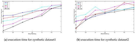
Figure 4. Comparative analysis of execution time (s) for synthetic datasets.

The evaluation metrics such as min-value, max-value, upper (25%), middle (50%) and lower (75%) quartile values have been listed in Table 3. $NMI$ value provided by the CDSW algorithm at each point in the box plot is observed to be better. It may be observed that the Walktrap algorithm performs close to the proposed algorithm with respect to the $NMI$ metric. Modularity metric indicates the quality of community partition.

Table 3. Box plot statistics for modularity, $NMI$ and F-measure.

	Modularity					$\mathit{NMI}$					F-Measure
	MIN	25%	50%	75%	MAX	MIN	25%	50%	75%	MAX	MIN	25%	50%	75%	MAX
INF	0.46	0.59	0.73	0.81	0.86	0.54	0.68	0.75	0.81	0.92	0.57	0.72	0.76	0.83	0.93
SG	0.46	0.6	0.72	0.79	0.83	0.58	0.7	0.76	0.82	0.93	0.58	0.72	0.78	0.85	0.92
GN	0.43	0.59	0.68	0.77	0.85	0.58	0.69	0.75	0.81	0.88	0.54	0.74	0.78	0.84	0.89
WT	0.49	0.61	0.69	0.81	0.84	0.59	0.71	0.79	0.83	0.92	0.56	0.75	0.78	0.83	0.89
CDSW	0.52	0.68	0.75	0.83	0.88	0.62	0.71	0.81	0.83	0.94	0.59	0.75	0.82	0.87	0.94

A t-test has been performed for static analysis of all mentioned community detection algorithms. Mean deviation and p-value have been extracted from the t-test. The mean deviation of evaluation metrics for all the algorithms are presented in Table 4. It may be noticed from Table 4 that the CDSW algorithm has positive deviation for all evaluation metrics, and it implies that it performs better with respect to all metrics. p-value in the t-test represents a significant difference of the CDSW algorithm with respect to other algorithms. Table 5 lists the statistics of p-value between all algorithms. An algorithm is said to be significantly different from others if its p-value is less than 0.05. It can be further noticed from Table 5, that p-value for the proposed algorithm in all of the evaluation metrics is less than 0.05. From this observation, it may be inferred that the CDSW algorithm is significantly different from all other algorithms with respect to metrics considered for comparison.

Table 4. Mean deviation in modularity, $NMI$ and F-measure for different algorithms.

	Modularity					$\mathit{NMI}$					F-Measure
	INF	SG	GN	WT	CDSW	INF	SG	GN	WT	CDSW	INF	SG	GN	WT	CDSW
INF	0.000	−0.010	−0.002	−0.028	−0.042	0.000	−0.010	−0.002	0.028	−0.042	0.000	−0.005	−0.006	−0.009	−0.036
SG	0.010	0.000	0.008	−0.018	−0.032	0.010	0.000	0.008	−0.018	−0.032	0.005	0.000	−0.001	−0.003	−0.030
GN	0.002	−0.008	0.000	−0.026	−0.040	0.002	−0.008	0.000	−0.026	−0.040	0.006	0.001	0.000	−0.003	−0.029
WT	0.028	0.018	0.026	0.000	−0.014	0.028	0.018	0.026	0.000	−0.014	0.009	0.003	0.003	0.000	−0.027
CDSW	0.042	0.032	0.040	0.014	0.000	0.042	0.032	0.040	0.014	0.000	0.036	0.030	0.029	0.027	0.000

Table 5. p-value obtained from t-test for modularity, $NMI$ and F-measure.

	Modularity					$\mathit{NMI}$					F-Measure
	INF	SG	GN	WT	CDSW	INF	SG	GN	WT	CDSW	INF	SG	GN	WT	CDSW
INF	-	0.241	0.761	0.001	0.000	-	0.241	0.761	0.001	0.000	-	0.324	0.442	0.234	0.000
SG	0.241	-	0.203	0.008	0.000	0.241	-	0.203	0.008	0.000	0.324	-	0.875	0.562	0.000
GN	0.761	0.203	-	0.000	0.000	0.761	0.203	-	0.000	0.000	0.442	0.875	-	0.515	0.000
WT	0.001	0.008	0.000	-	0.015	0.001	0.008	0.000	-	0.015	0.234	0.562	0.515	-	0.000
CDSW	0.000	0.000	0.000	0.015	-	0.000	0.000	0.000	0.015	-	0.000	0.000	0.000	0.000	-

8. Threat to Validity

• In the proposed work, threshold value for similarity index has been considered to be 0.5. This work may have a validation threat when the threshold value for similarity index is chosen to be higher than 0.8.
• Hadoop framework has been used for distributing computation in multiple nodes where data has been stored in the HDFS file system. All the data present in the HDFS file system are immutable in nature. The proposed algorithm may not perform well when the social network is dynamic in nature i.e., the structure of the network changes in course of time. In future work, issues regarding community detection in the dynamic network may be resolved.

9. Conclusions

The community detection problem is one of the challenging ones in social network analysis. In this study, communities have been detected in a distributed manner in order to have lesser computation time. Large-scale networks always follow small world phenomenon, which is based on the six degrees of separation principle. In this paper, similarity value between every pair of nodes has been obtained based on the random walk up to 3rd walk length. From the experimental analysis, it is observed that the proposed algorithm i.e., CDSW, provides better performance based on values of modularity, NMI and F-measure as compared to a few other community detection algorithms referred to in literature. From t-test analysis, the proposed algorithm is observed to be significantly different from other algorithms. It also provides better performance in terms of execution time, especially when large-scale networks are considered.

For the sake of simplicity, we have implemented all the algorithms in the undirected network. However, the proposed algorithm can be extended to the directed network by carefully choosing the source node in the network. As the network is a directed one, the source node can’t be chosen randomly. The node with only the in-degree feature cannot be the source node for further processing. By imposing a constraint on choosing criteria for source node (i.e., source node must have at least one out-degree), the proposed algorithm can be extended to detect community for the directed network.

The proposed algorithm can be further extended to dynamic social networks, where a large number of nodes along with their relationships are added more frequently. In future, other distributed frameworks like Spark and Storm may be implemented in the community detection process, in order to have further improvement in execution time.

References

- Kossinets, G.; Watts, D.J. Empirical analysis of an evolving social network. Science 2006, 311, 88–90. [Google Scholar] [CrossRef] [PubMed]
- Carrington, P.J.; Scott, J.; Wasserman, S. Models and Methods in Social Network Analysis; Cambridge University Press: New York, NY, USA, 2005; Volume 28. [Google Scholar]
- Freeman, L.C. Centrality in social networks conceptual clarification. Soc. Netw. 1978, 1, 215–239. [Google Scholar] [CrossRef]
- Bakshy, E.; Rosenn, I.; Marlow, C.; Adamic, L. The role of social networks in information diffusion. In Proceedings of the 21st International Conference on World Wide Web, Lyon, France, 16–20 April 2012; pp. 519–528. [Google Scholar]
- Liben-Nowell, D.; Kleinberg, J. The link-prediction problem for social networks. J. Assoc. Inf. Sci. Technol. 2007, 58, 1019–1031. [Google Scholar] [CrossRef]
- Clauset, A.; Newman, M.E.J.; Moore, C. Finding community structure in very large networks. Phys. Rev. E 2004, 70, 066111. [Google Scholar] [CrossRef] [PubMed]
- Stephen, A.T.; Toubia, O. Explaining the power-law degree distribution in a social commerce network. Soc. Netw. 2009, 31, 262–270. [Google Scholar] [CrossRef]
- Newman, M.E.J.; Watts, D.J. Scaling and percolation in the small-world network model. Phys. Rev. E 1999, 60, 7332. [Google Scholar] [CrossRef]
- Borgatti, S.P.; Cross, R. A relational view of information seeking and learning in social networks. Manag. Sci. 2003, 49, 432–445. [Google Scholar] [CrossRef]
- Travers, J.; Milgram, S. The small world problem. Phychol. Today 1967, 1, 61–67. [Google Scholar]
- Behera, R.K.; Rath, S.K. An efficient modularity based algorithm for community detection in social network. In Proceedings of the International Conference on Internet of Things and Applications (IOTA), Pune, India, 22–24 January 2016; pp. 162–167. [Google Scholar]
- Shu, W.; Chuang, Y.-H. The perceived benefits of six-degree-separation social networks. Int. Res. 2011, 21, 26–45. [Google Scholar] [CrossRef]
- Newman, M.E.J. Detecting community structure in networks. Eur. Phys. J. B-Condens. Matter Complex Syst. 2004, 38, 321–330. [Google Scholar] [CrossRef]
- Behera, R.K.; Rath, S.K.; Jena, M. Spanning tree based community detection using min-max modularity. Procedia Comput. Sci. 2016, 93, 1070–1076. [Google Scholar] [CrossRef][Green Version]
- Newman, M.E.J.; Watts, D.J.; Strogatz, S.H. Random graph models of social networks. Proc. Natl. Acad. Sci. USA 2002, 99 (Suppl. 1), 2566–2572. [Google Scholar] [CrossRef] [PubMed]
- Kempe, D.; Kleinberg, J.; Tardos, É. Maximizing the spread of influence through a social network. In Proceedings of the Ninth ACM SIGKDD International Conference on Knowledge Discovery and Data Mining, Washington, DC, USA, 24–27 August 2003; pp. 137–146. [Google Scholar]
- Leskovec, J.; Mcauley, J.J. Learning to discover social circles in ego networks. In Proceedings of the Advances in Neural Information Processing Systems, Lake Tahoe, NV, USA, 3–6 December 2012; pp. 539–547. [Google Scholar]
- Newman, M.E.J. The structure and function of complex networks. SIAM Rev. 2003, 45, 167–256. [Google Scholar] [CrossRef]
- Chopade, P.; Zhan, J. Structural and functional analytics for community detection in large-scale complex networks. J. Big Data 2015, 2, 1–28. [Google Scholar]
- Cook, D.J.; Holder, L.B. Mining Graph Data; John Wiley & Sons: Hoboken, NJ, USA, 2006. [Google Scholar]
- Newman, M.E.J. Analysis of weighted networks. Phys. Rev. E 2004, 70, 61311–61319. [Google Scholar] [CrossRef] [PubMed]
- De Meo, P.; Ferrara, E.; Fiumara, G.; Provetti, A. Mixing local and global information for community detection in large networks. J. Comput. Syst. Sci. 2014, 80, 72–87. [Google Scholar] [CrossRef]
- Breiger, R.L.; Boorman, S.A.; Arabie, P. An algorithm for clustering relational data with applications to social network analysis and comparison with multidimensional scaling. J. Math. Psychol. 1975, 12, 328–383. [Google Scholar] [CrossRef]
- Gregory, S. Finding overlapping communities in networks by label propagation. New J. Phys. 2010, 12, 103018. [Google Scholar] [CrossRef]
- Pons, P.; Latapy, M. Computing communities in large networks using random walks. In Computer and Information Sciences-ISCIS 2005; Springer: Istanbul, Turkey, 2005; pp. 284–293. [Google Scholar]
- Eaton, E.; Mansbach, R. A spin-glass model for semi-supervised community detection. In Proceedings of the Twenty-Sixth AAAI Conference on Artificial Intelligence, Toronto, Ontario, Canada, 22–26 July 2012; pp. 900–906. [Google Scholar]
- Agreste, S.; De Meo, P.; Fiumara, G.; Piccione, G.; Piccolo, S.; Rosaci, D.; Sarné, G.M.L.; Vasilakos, A.V. An empirical comparison of algorithms to find communities in directed graphs and their application in web data analytics. IEEE Trans. Big Data 2017, 3, 289–306. [Google Scholar] [CrossRef]
- Sun, P.G.; Gao, L. A framework of mapping undirected to directed graphs for community detection. Inf. Sci. 2015, 298, 330–343. [Google Scholar] [CrossRef]
- Deng, X.; Zhai, J.; Lv, T.; Yin, L. Efficient vector influence clustering coefficient based directed community detection method. IEEE Access 2017, 5, 17106–17116. [Google Scholar] [CrossRef]
- Rosvall, M.; Bergstrom, C.T. Maps of random walks on complex networks reveal community structure. Proc. Natl. Acad. Sci. USA 2008, 105, 1118–1123. [Google Scholar] [CrossRef] [PubMed]
- Orman, G.K.; Labatut, V.; Cherifi, H. On accuracy of community structure discovery algorithms. arXiv, 2011; arXiv:1112.4134. [Google Scholar]
- Zhang, P.; Wang, J.; Li, X.; Li, M.; Di, Z.; Fan, Y. Clustering coefficient and community structure of bipartite networks. Phys. A Stat. Mech. Appl. 2008, 387, 6869–6875. [Google Scholar] [CrossRef]
- Kemeny, J.G.; Snell, J.L. Finite Markov Chains; Springer: Princeton, NJ, USA, 1960; Volume 356. [Google Scholar]
- McDaid, A.F.; Greene, D.; Hurley, N. Normalized mutual information to evaluate overlapping community finding algorithms. arXiv, 2011; arXiv:1110.2515. [Google Scholar]
- Leskovec, J.; Krevl, A. {SNAP Datasets}:{Stanford} Large Network Dataset Collection. Available online: http://snap.stanford.edu/data (accessed on 31 August 2015).
- Newman, M.E.J. Modularity and community structure in networks. Proc. Natl. Acad. Sci. USA 2006, 103, 8577–8582. [Google Scholar] [CrossRef] [PubMed]
© 2017 by the authors. Licensee MDPI, Basel, Switzerland. This article is an open access article distributed under the terms and conditions of the Creative Commons Attribution (CC BY) license (http://creativecommons.org/licenses/by/4.0/).