A Selective Dynamic Sampling Back-Propagation Approach for Handling the Two-Class Imbalance Problem

Abstract

In this work, we developed a Selective Dynamic Sampling Approach (SDSA) to deal with the class imbalance problem. It is based on the idea of using only the most appropriate samples during the neural network training stage. The “average samples”are the best to train the neural network, they are neither hard, nor easy to learn, and they could improve the classifier performance. The experimental results show that the proposed method is a successful method to deal with the two-class imbalance problem. It is very competitive with respect to well-known over-sampling approaches and dynamic sampling approaches, even often outperforming the under-sampling and standard back-propagation methods. SDSA is a very simple method for automatically selecting the most appropriate samples (average samples) during the training of the back-propagation, and it is very efficient. In the training stage, SDSA uses significantly fewer samples than the popular over-sampling approaches and even than the standard back-propagation trained with the original dataset.

1. Introduction

In recent years, the class imbalance problem has been a hot topic in machine learning and data-mining [1,2]. It appears when the classifier is trained with a dataset where the number of samples in one class is lower than the samples in the other class, this and produces an important deterioration in the classifier performance [3,4].

The common methods handled with the class imbalance problem have been the re-sampling methods (under-sampling and over-sampling) [2,5,6], mainly due to the independence of the underlying classifier [7]. One of the most well-known over-sampling methods is the Synthetic Minority Over-sampling Technique (SMOTE). This generates artificial samples of the minority class by interpolating existing instances that lie close together [8]. The development of other samplings has been motivated: borderline-SMOTE, Adaptive Synthetic Sampling (ADASYN), SMOTE editing nearest neighbor, safe-level-SMOTE, Density-Based Synthetic Minority Over-sampling TEchnique (DBSMOTE), SMOTE + Tomek’s Links [9], among others (see [1,7,10]).

An interest has been observed for finding the best samples to build the classifiers. For example, borderline-SMOTE has been proposed to over-sample only the minority samples near the class decision borderline [11]. Accordingly, in [12], the safe-level-SMOTE is proposed, to select minority class instances from the safe level region, and then, these samples are used to generate synthetic instances. ADASYN has been developed to generate more synthetic data from minority class samples that are harder to learn than those from minority class samples, which are easy to learn [13]. In a similar way, SPIDER approaches (framework that integrates a selective data pre-processing with the Ivotes ensemble method) over-sampling locally only for those minority class samples that are difficult to learn and includes a removing or relabeling process of noisy samples from the majority class [14,15]. The above discussed approaches have in common that they use the K nearest neighbors rule as the basis, and they are applied before the classifier training stage.

On the other hand, the under-sampling methods have shown effectiveness to deal with the class imbalance problem (see [7,8,10,16,17,18,19])). One of the most successful under-sampling methods has been the random under-sampling, which eliminates random samples from the original dataset (usually from the majority class) to decrease the class imbalance, however, this method loses effectiveness when removing significant samples [7]. Other important under-sampling methods including a heuristic mechanism are: the neighborhood cleaning rule, from Wilson editing [20], one-sided selection [21], Tomek links [22] and the Condensed Nearest Neighbor rule (CNN) [23]. Basically, the aim of the cleaning mechanism is: (i) to eliminate samples with a high likelihood of being noise or atypical samples or (ii) to eliminate redundant samples in CNN methods. In the same way as the above approaches, we apply these methods before the training process. They employ the K nearest neighbors rule (except the Tomek links methods) as the basis.

Another important alternative to face the class imbalance has been the Cost Sensitive (CS) approach, which has become one of the most relevant topics in machine learning research in recent years [24]. They consider the costs associated with misclassifying samples, i.e., CS methods use different cost matrices describing the costs for misclassifying any particular data sample [10]. The over- and under-sampling could be a special case of the CS techniques [25]. Anther CS method is threshold-moving, which moves the output threshold toward inexpensive classes, such that samples with higher costs become hard to misclassify. It is applied in the test phase and does not affect the training phase [24].

Ensemble learning is an effective method that has increasingly been adopted to combine multiple classifiers and class imbalance approaches to improve the classification performance [2,4,5]. In order to combine the multiple classifiers, it is common to use the hard and soft ensemble. The former uses binary votes, while the latter uses real-valued votes [26].

Recently, dynamic sampling methods have become an interesting way to deal with the class imbalance problem. They are attractive, because they automatically find the proper sampling amount for each class in the training stage (different from conventional strategies as over- and/or under-sampling techniques). In addition, some dynamic sampling methods also identify the “best samples” for classifier training. For example, Lin et al. [27] propose a dynamic sampling method with the ability to identify samples with a high probability to be misclassified. The idea is that the classifier trained with these samples may produce better classification results. Other methods that can be considered as dynamic sampling are: (i) the snowball method (proposed in [28] and used as a dynamic training method in [29,30]); (ii) the genetic dynamic training technique [31,32]; in it, the authors employ a genetic algorithm to find the best over-sampling ratio; (iii) the mean square error (MSE) dynamic over-sampling method [19], which is based on the MSE back-propagation for automatically identifying the over-sampling rate. Chawla et al. [33] present a WRAPPER paradigm (for which the search is guided by the classification goodness measure as score) to discover the amount of the under-sampling and over-sampling rate for a dataset. Debowski et al. [34] show a very similar work.

The dynamic sampling approaches are a special case of the sampling techniques. The main difference of these methods with respect to the conventional sampling strategies is in the time when they sample the data or when they select the examples to be sampled (see [19,27,28,31,32]).

In this paper, a Selective Dynamic Sampling Approach (SDSA) to deal with the two-class imbalance problem is presented. This method is useful to find automatically the appropriate sampling amount for each class through the selection of the “best samples” to train the multilayer perceptron with the back-propagation algorithm [35]. The proposed method was tested over thirty five real datasets and compared to some state-of-the-art class imbalance approaches.

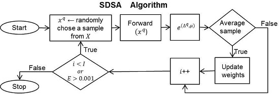
2. Selective Dynamic Sampling Approach

Researchers in the class imbalance problem have shown their interest in finding the best samples to build the classifiers, for example eliminating those samples with a high probability to be noise or overlapped samples [18,36,37,38,39,40], or focusing on those close to the borderline decision [11,13,41] (the latter has been less explored).

In accordance with the above discussion, three categories of samples can be basically identified in the class imbalance literature:

• Noise and rare or outlier samples. The first ones are instances with error in their labels [7] or erroneous values in the features that describe them, and the last ones are the minority and rare samples located inside the majority class [42].
• Border or overlapped samples are those samples located where the decision boundary regions intersect [18,38].
• Safe samples are those with a high probability of being correctly labeled by the classifier, and they are surrounded by samples of the same class [42].

Nevertheless, those samples situated close to the borderline decision and far from the safe samples might be of interest; in other words, those that are neither hard nor easy to learn. These samples are called “average samples” [35].

In this section, a Selective Dynamic Sampling Approach (SDSA) to train the multilayer perceptron is presented. The aim of this proposal is to deal with the two-class imbalance problem, i.e., this method only works with two-class imbalanced datasets. This SDSA is based on a modification of the “stochastic” back-propagation algorithm and derived from the idea of using average samples to train Arificial Neural Networks (ANN), in order to try to improve the classifier performance. The proposed method consists of two steps, and it is described below:

• Before training: The training dataset is balanced 100% through an effective over-sampling technique. In this work, we use the SMOTE [8] (SDSAS) and random over-sampling (SDSAO) [16].
• During training: The proposed method selects the average samples to update the neural network weights. From the balanced training dataset, it chooses average samples to use in the neural network training. With the aim to identify the average samples, we propose the next function:

  $$\gamma \left({\Delta }^q\right)=exp(-\frac{\left|\right|{\Delta }^q-\mu {\left|\right|}^2}{2{\sigma }^2})$$

  (1)

  Variable ${\Delta }^q$ is the normalized difference amongst the real neural network outputs for a sample q,

  $${\Delta }^q=\frac{z_0^q}{\sqrt{{(z_0^q-z_1^q)}^2}}-\frac{z_1^q}{\sqrt{{(z_0^q-z_1^q)}^2}}$$

  (2)

  where $z_0^q$ and $z_1^q$ are respectively the real neural network outputs corresponding to a q sample. The ANN only has two neural network outputs ($z_0^q$ and $z_1^q$), because it has been designed to work with datasets of two classes [43].

The Selective Dynamic Sampling Approach (SDSA) is detailed in Algorithm 1, where $t_j^{\left(q\right)}$ and $z_j^{\left(q\right)}$ are the desired and real neural network outputs for a sample q, respectively.

Algorithm 1 The Selective Dynamic Sampling Approach (SDSA) based on the stochastic back-propagation multilayer perceptron.

Input: X (input dataset), N (number of features in X), K (number of classes in X), Q (number of samples in X), M (number of middle neurodes), J (number output neurodes), I number of iterations and learning rate η. Output: the weights w $=(w_{11},w_{21},...,w_{NM})$ u $=(u_{11},u_{21},...,w_{MJ})$. INIT( ): 1: Read MLP file ($X,N,M,J,Q,I$ and η); 2: Generate initial weights randomly between $-0.5$ and $0.5$; LEARNING( ): 3: while $i<I$ or $E>0.001$ do 4:    $x^q\leftarrow$ randomly chose a sample from X 5:    FORWARD($x^q$); 6:    ${\Delta }^q=(z_0^q/\sqrt{{(z_0^q-z_1^q)}^2})-(z_1^q/\sqrt{{(z_0^q-z_1^q)}^2})$; 7:    $\gamma ({\Delta }^q)=exp(-||{\Delta }^q-{\mu \left|\right|}^2/2{\sigma }^2)$; 8:    if Random( ) $<=\gamma \left({\Delta }^q\right)$ then 9:       UPDATE($x^q$); 10:    end if 11:    $i++$; 12: end while FORWARD($x^q$): 13: for $m=0$ to $m<M$ do 14:    for $n=0$ to $n<N$ do 15:       $y_m\leftarrow y_m+x_n^q*w_{nm}$; 16:    end for 17:    $y_m=net\left(y_m\right)$; 18: end for 19: for $j=0$ to $j<J$ do 20:    for $m=0$ to $m<M$ do 21:       $z_j\leftarrow z_j+u_{mj}*y_m$; 22:    end for 23:    $z_j\leftarrow net\left(z_j\right)$; 24: end for UPDATE($x^q$): 25: for $m=1$ to M do 26:    for $j=1$ to J do 27:       $u_{mj}^{r+1}\leftarrow$$u_{mj}^r+\eta \{(t_j^{\left(q\right)}-z_j^{\left(q\right)})[z_j^{\left(q\right)}(1-z_j^{\left(q\right)})]y_m^{\left(q\right)}\}$; 28:    end for 29:    for $n=1$ to N do 30:       $w_{nm}^{r+1}\leftarrow$$w_{nm}^r+\eta \{{\sum }_{j=1,J}(t_j^{\left(q\right)}-z_j^{\left(q\right)})[z_j^{\left(q\right)}(1-z_j^{\left(q\right)})]u_{mj}^{\left(r\right)}\}{x}_n[y_m^{\left(q\right)}(1-y_m^{\left(q\right)})][x_n^{\left(q\right)}]$; 31:    end for 32: end for

2.1. Selecting μ Values

The appropriate selection of the variable μ is critical to select the average samples or other kind of samples (border or safe samples [42]). Variable μ is computed under the following consideration: the target ANN outputs ($t_j$) are usually codified in zero and one values [43]. For example, for a two-class problem (Class A and Class B), the desired ANN outputs are codified as $(1,0)$ and $(0,1)$ for Classes A and B, respectively. These values are the target ANN outputs ($t_j$), i.e., the desired final values emitted by the ANN after training. In accordance with this understanding, the expected μ values are:

• $\mu \approx$ 1.0 for safe samples. It is expected that ANN classifies with a high accuracy level, i.e., it is expected that the real ANN outputs for all neurons ($z_j$) will be values close to (1, 0) and (0, 1) for Classes A and B, respectively. Whether we apply Equation (2), the expected value is 1.0, at which the γ function has its maximum value.
• $\mu \approx$ 0.0 for border samples. It is expected that the classifier misclassifies. The expected ANN outputs for all neurons are values close to (0.5, 0.5), then the Δ is approximately 0.0, at which the γ function has its maximum value for these samples.
• $\mu \approx$ 0.5 for average samples. It is expected that ANN classifies correctly, but with less accuracy. In addition, the average samples are between safe ($\mu \approx 1.0$) and border ($\mu \approx 0.0$) samples.

The recommended μ values to select the average samples are those around 0.5. An independent validation set to find the most appropriate μ value is proposed to avoid any bias in the testing process.

For this independent validation, a minimal subset from the training data is used. Firstly, the ten-fold cross-validation for each dataset is applied (Section 5.1); next, only 10% of samples are randomly taken from each training fold (${\mathrm{TF}}^{10}$), then ${\mathrm{TF}}^{10}$ is split into two disjoints folds of the same size (${\mathrm{TF}}_{train}^5$ and ${\mathrm{TF}}_{test}^5$, respectively). Next, the proposed method (SDSA) is applied over the ${\mathrm{TF}}_{train}^5$ and ${\mathrm{TF}}_{test}^5$ to find the best μ value. The tested values for μ were 0.25, 0.375, 0.5, 0.625 and 0.75. Finally, the μ value, for which the best Area Under the Curve (AUC) [44] rank was obtained, is chosen by SDSA on ${\mathrm{TF}}^{10}$.

Note that this independent validation does not imply an important computational cost, because it only uses 10% of the training data to find the most appropriate μ value. This independent validation unbiased the performance on the testing data process, due to the test data not being used.

3. State-of-the-Art of the Class Imbalance Approaches

In the state-of-the-art class imbalance problem, the over- and under-sampling methods are very popular and successful approaches to deal with this problem (see [7,8,10,16,17,18,19]). Over-sampling replicates samples in the minority-class, and under-sampling eliminates samples from the majority-class, biasing the discrimination process to compensate for the class imbalance.

This section describes some well-known sampling approaches that have been effectively applied to deal with the class imbalance problem. These approaches are used with the aim to compare the classification performance of the proposed method with respect to the state-of-the-art of class imbalance approaches.

3.1. Under-Sampling Approaches

TL Tomek links are pairs of samples a and b from different classes, and there does not exist a sample c, such that $d(a,c)<d(a,b)$ or $d(b,c)<d(a,b)$, where d is the distance between pairs of samples [22]. Samples in TL are noisy or lie in the decision border. This method removes those majority class samples belonging to TL [9].

CNN The main goal of the condensed nearest neighbor algorithm is the reduction of the size of the stored dataset of training samples while trying to maintain (or even improve) generalization accuracy. In this method, every member of X (the original training dataset) must be closer to a member of S (the pruned set) of the same class than any other member of S from a different class [23].

CNNTL combines the CNN with TL [9].

NCL The Neighborhood Cleaning Rule uses the Editing Nearest Neighbor (ENN) rule, but only eliminates the majority class samples. ENN uses the $k-NN$$(k>1)$ classifier to estimate the class label of every sample in the dataset and discards those samples whose class labels disagree with the class associated with the majority of the k neighbors [20].

OSS The One-Sided Selection method performs TL, then CNN on the training dataset [21].

RUS The Random Under-Sampling randomly eliminates samples from the majority class and biases the discrimination process to compensate for the class imbalance.

3.2. Over-Sampling Approaches

ADASYN is an extension of SMOTE, creating more samples in the vicinity of the boundary among the two classes than in the interior of the minority class [13].

ADOMS The Adjusting the Direction Of the synthetic Minority clasS method, setting the direction of the synthetic minority class samples, this works like SMOTE, but it generates synthetic examples along the first component of the main axis of the local data distribution [45].

ROS The Random Over-Sampling duplicates samples randomly from the minority class, biasing the discrimination process to compensate for the class imbalance.

SMOTE [8] generates artificial samples of the minority class by interpolating existing instances that lie close together. It finds the k intra-class nearest neighbors for each minority sample, and then, synthetic samples are generated in the direction of some or all of those nearest neighbors.

B-SMOTE Borderline-SMOTE [11] selects samples from the minority class that are on the borderline (of the minority decision region, in the feature space) and only performs SMOTE on those samples, instead of over-sampling all or taking a random subset.

SMOTE-ENN This technique consists of applying the SMOTE and then applying the ENN rule [9].

SMOTE-TL is the combination of SMOTE and TL [9].

SL -SMOTE Safe-Level SMOTE is based on the SMOTE, but it generates synthetic minority class samples positioned closer to the largest safe level; then, all synthetic samples are only generated in safe regions [12].

SPIDER-1 is an approach that combines a local over-sampling of those minority class samples that are difficult to learn with removing or relabeling noisy samples from the majority class [14].

SPIDER-2 The major difference between this method and SPIDER-1 is that it divides into two stages the pre-processing of the majority and minority class samples, i.e., first pre-processing the majority class samples and next the minority class samples (considering the changes introduced in the first stage) [15].

4. Dynamic Sampling Techniques to Train Artificial Neural Networks

Dynamic sampling techniques have become an interesting way to deal with the class imbalance problem on the Multilayer Perceptron (MLP) trained with stochastic back-propagation [19,27,28,31,32]. Different from conventional strategies as over- and/or under-sampling techniques, the dynamic sampling finds automatically in the training stage the properly sampling amount for each class for dealing with the class imbalance problem. In this section, we present some details and the main features of two dynamic sampling methods.

4.1. Method 1. Dynamic Sampling

The basic idea of the Dynamic Sampling (DyS) method, proposed in [27], is to design a simple DyS that dynamically selects samples during the training process. In this method, a pre-deletion of any sample to prevent information loss, to dynamically select the samples (hard to classify) to train the ANN and to make the best use of the dataset does not exist. According to this main idea, the general steps in each epoch can be described as follows.

• Randomly fetch a sample q from the training dataset.
• Estimate the probability p that the example should be used for the training.

  $$p=\left\{\begin{array}{cc}1,\hfill & \text{if}\delta \le 0\\ exp(-\delta ·r_j/min\left\{r_i\right\}),\hfill & \text{otherwise},\end{array}\right.$$

  (3)

  where $\delta =z_j^q-ma{x}_{i\ne c}\left\{z_i^q\right\}$. $z_i^q$ is the i-th real ANN output of the sample q and j is the class label to which q belongs. $r_c=Q_c/Q$ is the class ratio; $Q_c$ is the number of samples belonging to class c; and Q is the sample number.
• Generate a uniform random real number μ between zero and one.
• If $\mu <p$, then use the sample q to update the weights by the back-propagation rules.
• Repeat Steps 1–4 on all samples of the training dataset in each training epoch.

In addition, the authors of the paper [27] use an over-sampling method based on a heuristic technique to avoid bias for the class imbalance problem. Beginning with the first epoch, the process consists of the samples of all classes, except the largest classes over-sampled to make the dataset balanced. As the training process goes on, the over-sampling ratio (ρ) is attenuated in each epoch ($ep$) by a heuristic technique (Equation (4)). It is calculated as:

$$\rho =(r_{max}/r_j)/ln\left(ep\right)$$

(4)

where $ep$ $(>2)$ and $max$ represent the largest majority class.

4.2. Method 2. Dynamic Over-Sampling

In [19], a Dynamic Over-Sampling (DOS) technique to deal with the class imbalance problem was proposed. The main idea of DOS is to balance the MSE on the training stage (when a multi-class imbalanced dataset is used) through an over-sampling technique. Basically, the DOS method consists of two steps:

• Before training: The training dataset is balanced at 100% through an effective over-sampling technique. In this work, SMOTE [8] is utilized.
• During training: The MSE by class $E_j$ is used to determine the number of samples by class (or class ratio) in order to forward it to the ANN. The equation employed to obtain the class ratio is defined as:

  $${\mathit{ratio}}_j=\frac{E_{max}}{E_j}\times \frac{Q_j}{Q_{max}};\mathit{for}j=1,2,...,J$$

  (5)

  where J is the number of classes in the dataset and $max$ identifies the largest majority class. Equation (5) allows balancing the MSE by class, reducing the impact of the class imbalance problem on the ANN.

The DOS method only uses the necessary samples for dealing with the class imbalance problem and, in this way, to avoid getting a poor classifications performance as a result of training the ANN with imbalanced datasets.

5. Experimental Set-Up

In this section, the techniques, datasets and experimental framework used in this paper are to be described.

5.1. Database Description

Firstly, for the experimental stage, five real-world remote sensing databases are chosen: Cayo, Feltwell, Satimage, Segment and 92AV3C.The Cayo dataset comes from a particular region in the Gulf of Mexico [18]. The Feltwell dataset represents an agricultural area near the village of Feltwell (UK) [46]. The Satimage and Segment datasets are from the UCI (University of California, Irvine) Machine Learning Database Repository [47]. The 92AV3C dataset [48] corresponds to a hyperspectral image (145 × 145 pixels, 220 bands, 17 classes) taken over the Northwestern Indiana Indian Pines by the AVIRIS (Airborne Visible / Infrared Imaging Spectrometer) sensor. In this work, we employed a reduced version of this dataset with six classes (2, 3, 4, 6, 7 and 8) and thirty eight attributes as in [18].

The two-class imbalance problem is only studied. We decompose the multi-class problems into multiple two-class imbalanced problems. This proceeds as follows: one class ($c_j$) is taken from the original database ($DB$) to integrate the minority class ($c^{+}$), and the rest of classes were joined to shape the majority class ($c^{-}$). Then, we integrate the two-class database $D{B}_j$ ($j=1,2,...,J$, and J is the number of classes in $DB$). In other words, $D{B}_j=c^{+}\cup c^{-}$. Therefore, for each database, J two-class imbalanced datasets were obtained. The main characteristics of the new produced benchmarking datasets are shown in

Table 1. A brief summary of the main characteristics of the new produced benchmarking dataset.

Dataset	# of Features	# of Minority Classes Samples	# of Majority Class Samples	Imbalance Ratio
CAY0	4	838	5181	6.18
CAY1	4	293	5726	19.54
CAY2	4	624	5395	8.65
CAY3	4	322	5697	17.69
CAY4	4	133	5886	44.26
CAY5	4	369	5650	15.31
CAY6	4	324	5695	17.58
CAY7	4	722	5297	7.34
CAY8	4	789	5230	6.63
CAY9	4	833	5186	6.23
CAY10	4	772	5247	6.80
FELT0	15	3531	7413	2.10
FELT1	15	2441	8503	3.48
FELT2	15	896	10,048	11.21
FELT3	15	2295	8649	3.77
FELT4	15	1781	9163	5.14
SAT0	36	1508	4927	3.27
SAT1	36	1533	4902	3.20
SAT2	36	703	5732	8.15
SAT3	36	1358	5077	3.74
SAT4	36	626	5809	9.28
SAT5	36	707	5728	8.10
SEG0	19	330	1140	3.45
SEG1	19	50	1420	28.40
SEG2	19	330	1140	3.45
SEG3	19	330	1140	3.45
SEG4	19	50	1420	28.40
SEG5	19	50	1420	28.40
SEG6	19	330	1140	3.45
92A0	38	190	4872	25.64
92A1	38	117	4945	42.26
92A2	38	1434	3628	2.53
92A3	38	2468	2594	1.05
92A4	38	747	4315	5.78
92A5	38	106	4956	46.75

. This table shows that the datasets used in this work have several class imbalance levels (see the class imbalance ratio), ranging from a low to a high class imbalance ratio (for example, see 92A3 and CAY4 datasets). In addition, the ten-fold cross-validation method was applied on all datasets shown in this table.

5.2. Parameter Specification for the Algorithms Employed in the Experimentation

The stochastic back-propagation algorithm was used in this work (the source code of back-propagation algorithm and the approaches (dynamic sampling methods) and the datasets used in this work are available at Ref. [49]), and for each training process, the weights were ten times randomly initialized. The learning rate (η) was set to $0.1$, and we established the stopping criterion at 500 epochs or if the MSE value is lower than $0.001$. A single hidden layer was used. The number of neurons in the hidden layer was set to four for every experiment.

All sampling methods (except ENN, SPIDER-1 and SPIDER-2, which employ three) use five nearest neighbors (if applicable) and sampling the training dataset to reach to relative class distribution balance (if applicable). ADASYN and ADOMS use the Euclidean distance, and the rest of the methods employ the Heterogeneous Value Difference Metric (HVDM) [50], if applicable. SPIDER-1 applies a weak amplification pre-processing option, and SPIDER-2 employs relabeling of noisy samples from the majority class and an amplification option. The sampling methods have been done using the KEEL [51].

In order to identify the most suitable value for the variable μ, an independent validation set to avoid any bias in the performance on the testing data is considered, meaning that the testing data for this validation are not used (see Section 2.1). Thereafter, the most appropriate value for the variable μ obtained for the datasets used in this work (Table 1) is $0.375$. The results presented in this paper were obtained with $\mu =0.375$. In addition, for this independent validation, only 200 epochs are used in the neural network training stage and about 8% of the samples of each dataset. This does not imply an important additional computational effort. The SDSAO and SDSAS methods are the proposed methods using ROS and SMOTE, respectively (see Section 4).

5.3. Classifier Performance and Significant Statistical Test

The Area Under the receiver operating characteristic Curve (AUC) [44] was used as the criteria of measure for the classifiers performance. It is one of the most widely-used and accepted techniques for the evaluation of binary classifiers in class imbalance domains [10].

Additionally, in order to strengthen the results analysis, a non-parametric statistical test is achieved. The Friedman test is a non-parametric method in which the first step is to rank the algorithms for each dataset separately; the best performing algorithm should have rank as 1, the second best rank as 2, etc. In case of ties, average ranks are computed. The Friedman test uses the average rankings to calculate the Friedman statistic, which can be computed as,

$${\chi }_F^2=\frac{12N}{K(K+1)}(\sum _j{R}_j^2-\frac{K{(K+1)}^2}{4})$$

(6)

K denotes the number of methods; N is the number of data sets; and $R_j$ is the average rank of method j on all datasets.

On the other hand, Iman and Davenport [52] demonstrated that ${\chi }_F^2$ has a conservative behavior. They proposed a better statistic (Equation (7)) distributed according to the $F-$distribution with $K-1$ and $(K-1)(N-1)$ degrees of freedom,

$$F_F=\frac{(N-1){\chi }_F^2}{N(K-1)-{\chi }_F^2}$$

(7)

In this work, the Friedman and Iman–Davenport tests are employed with the $\gamma =0.05$ level of confidence, and KEEL software [51] is utilized.

In addition, when the null-hypothesis was rejected, a post-hoc test is used in order to find the particular pairwise method comparisons producing statistically-significant differences. The Holm–Shaffer post-hoc tests are applied in order to report any significant difference between individual methods. The Holm procedure rejects the hypotheses ($H_i$) one at a time until no further rejections can be done [53]. To accomplish this, the Holm method ordains the p-values from the smallest to the largest, i.e., $p_1$≤$p_2$$\le p_{k-1}$, corresponding to the hypothesis sequence $H_1,H_2,...,H_{k-1}$. Then, the Holm procedure rejects $H_1$ to $H_{i-1}$ if i is the smallest integer, such that $p_i\le \alpha /(k-i)$. This procedure starts with the most significant p-value. As soon as a certain null-hypothesis cannot be rejected, all of the remaining hypotheses are retained, as well [54]. The Shaffer method follows a very similar procedure to that proposed by Holm, but instead of rejecting $H_i$ if $p_i\le \alpha /(k-i)$, it rejects $H_i$ if $p_i\le \alpha /t_i$, where $t_i$ is the maximum number of hypotheses that can be true given that any $(i-1)$ hypotheses are false [55].

6. Experimental Results and Discussion

In order to assess the performance of the proposed methods (SDSAO and SDSAS), a set of experiments has been carried out, over thirty five two-class datasets (Table 1) with ten well-known over-sampling approaches (ADASYN, ADOMS, B-SMOTE, ROS, SMOTE, SMOTE-ENN, SMOTE-TL, SPIDER-1, SPIDER-2 and SL-SMOTE), six popular under-sampling methods (TL, CNN, CNNTL, NCL, OSS and RUS) (for more detail about these re-sampling techniques, see Section 3) and two dynamic sampling approaches (DyS and DOS).

This section is organized as follows: First, the AUC values are shown, and the Friedman ranks are used to analyze the classification results (

Table 2. Back-propagation classification performance using the Area Under the receiver operating characteristic Curve (AUC) . The results represent the averaged values between ten folds and the initialization of ten different weights of the neural network. The best values are underlined in order to highlight them. ROS, Random Over-Sampling; SDSAO, Selective Dynamic Sampling Approach using ROS; DyS, Dynamic Sampling; SDSAS, Selective Dynamic Sampling Approach applying SMOTE; SMOTE-TL, SMOTE and TL;SMOTE, Synthetic Minority Over-sampling Technique; SL-SMOTE, Safe-Level SMOTE; SMOTE-ENN, SMOTE and Editing Nearest Neighbor (ENN) rule; ADOMS, Adjusting the Direction Of the synthetic Minority clasS method; B-SMOTE, Borderline-SMOTE; DOS, Dynamic Over-Sampling; RUS, Random Under-Sampling; ADASYN, Adaptive Synthetic Sampling; SPIDER 1 and 2, frameworks that integrate a selective data pre-processing with an ensemble method; NCL, Neighborhood Cleaning Rule; TL, Tomek links method; STANDARD, back-propagation without any pre-processing; OSS, One-Sided Selection method; CNN, Condensed Nearest Neighbor; CNNTL, Condensed Nearest Neighbor with TL (for more details see Section 3 and Section 4).

DATA	ROS	SDSAO	DyS	SDSAS	SMOTE-TL	SMOTE	SL-SMOTE	SMOTE-ENN	ADOMS	B-SMOTE	DOS	RUS	ADASYN	SPIDER-1	SPIDER-2	NCL	TL	STANDARD	OSS	CNN	CNNTL
CAY0	0.976	0.986	0.985	0.978	0.976	0.976	0.976	0.976	0.977	0.968	0.984	0.970	0.967	0.937	0.938	0.937	0.936	0.933	0.803	0.833	0.795
CAY1	0.969	0.979	0.975	0.968	0.969	0.969	0.970	0.970	0.970	0.966	0.985	0.955	0.965	0.735	0.789	0.745	0.717	0.752	0.931	0.916	0.918
CAY2	0.968	0.959	0.958	0.967	0.969	0.968	0.968	0.969	0.968	0.968	0.952	0.959	0.964	0.952	0.957	0.952	0.952	0.949	0.961	0.960	0.958
CAY3	0.985	0.985	0.983	0.981	0.986	0.985	0.984	0.985	0.984	0.973	0.991	0.950	0.975	0.948	0.949	0.940	0.929	0.941	0.809	0.826	0.839
CAY4	0.974	0.994	0.991	0.971	0.971	0.968	0.971	0.968	0.968	0.964	0.962	0.922	0.967	0.914	0.936	0.888	0.865	0.846	0.946	0.934	0.956
CAY5	0.952	0.922	0.956	0.943	0.952	0.950	0.949	0.951	0.951	0.950	0.908	0.933	0.951	0.781	0.834	0.773	0.769	0.772	0.666	0.618	0.617
CAY6	0.980	0.956	0.956	0.980	0.981	0.981	0.980	0.982	0.980	0.969	0.956	0.960	0.973	0.946	0.946	0.952	0.949	0.830	0.850	0.787	0.875
CAY7	0.991	0.983	0.983	0.990	0.990	0.990	0.991	0.991	0.991	0.983	0.986	0.988	0.967	0.986	0.985	0.984	0.984	0.985	0.776	0.824	0.788
CAY8	0.975	0.937	0.935	0.966	0.976	0.972	0.971	0.972	0.970	0.964	0.923	0.925	0.958	0.933	0.933	0.935	0.934	0.935	0.817	0.826	0.825
CAY9	0.915	0.923	0.920	0.910	0.917	0.916	0.915	0.915	0.916	0.911	0.898	0.896	0.909	0.875	0.868	0.860	0.848	0.834	0.879	0.849	0.872
CAY10	0.967	0.979	0.965	0.968	0.963	0.968	0.968	0.969	0.968	0.965	0.973	0.885	0.970	0.883	0.902	0.860	0.877	0.922	0.833	0.786	0.808
FELT0	0.979	0.982	0.980	0.979	0.978	0.978	0.977	0.977	0.978	0.971	0.977	0.977	0.951	0.976	0.976	0.977	0.976	0.977	0.952	0.955	0.937
FELT1	0.976	0.966	0.98	0.975	0.976	0.973	0.975	0.976	0.976	0.968	0.971	0.970	0.958	0.964	0.964	0.965	0.964	0.965	0.947	0.946	0.945
FELT2	0.976	0.947	0.960	0.976	0.974	0.975	0.976	0.974	0.975	0.959	0.969	0.959	0.963	0.914	0.921	0.918	0.901	0.890	0.952	0.948	0.948
FELT3	0.977	0.984	0.987	0.978	0.977	0.978	0.977	0.977	0.978	0.968	0.987	0.971	0.956	0.974	0.975	0.969	0.971	0.970	0.964	0.966	0.962
FELT4	0.983	0.992	0.976	0.985	0.983	0.983	0.984	0.983	0.983	0.977	0.988	0.981	0.964	0.968	0.972	0.972	0.968	0.968	0.968	0.969	0.961
SAT0	0.920	0.910	0.916	0.917	0.915	0.915	0.916	0.914	0.916	0.918	1.000	0.913	0.907	0.909	0.912	0.909	0.894	0.881	0.899	0.881	0.865
SAT1	0.985	0.988	0.988	0.984	0.986	0.983	0.986	0.984	0.985	0.983	0.996	0.983	0.976	0.983	0.983	0.982	0.982	0.981	0.982	0.981	0.976
SAT2	0.981	0.989	0.983	0.980	0.982	0.980	0.981	0.983	0.980	0.977	0.961	0.980	0.969	0.977	0.980	0.977	0.976	0.976	0.971	0.966	0.964
SAT3	0.961	0.965	0.958	0.960	0.958	0.962	0.962	0.961	0.963	0.960	0.911	0.957	0.955	0.957	0.958	0.950	0.955	0.943	0.954	0.956	0.945
SAT4	0.857	0.867	0.803	0.863	0.866	0.849	0.858	0.858	0.858	0.844	1.000	0.844	0.854	0.746	0.779	0.792	0.757	0.581	0.769	0.711	0.776
SAT5	0.944	0.945	0.928	0.925	0.944	0.944	0.944	0.942	0.941	0.920	1.000	0.917	0.913	0.847	0.823	0.855	0.853	0.842	0.927	0.921	0.927
SEG0	0.998	0.965	0.970	0.995	0.993	0.994	0.996	0.992	0.988	0.997	0.895	0.995	0.993	0.993	0.992	0.994	0.993	0.994	0.994	0.993	0.994
SEG1	1.000	1.000	1.000	1.000	1.000	1.000	1.000	1.000	0.988	1.000	0.991	0.999	1.000	1.000	1.000	0.999	0.999	1.000	0.925	0.909	0.914
SEG2	0.978	0.979	0.996	0.979	0.975	0.977	0.979	0.974	0.977	0.981	0.983	0.978	0.965	0.982	0.983	0.981	0.980	0.977	0.965	0.964	0.963
SEG3	0.973	0.967	0.976	0.963	0.971	0.973	0.972	0.970	0.911	0.971	0.952	0.961	0.961	0.969	0.966	0.970	0.974	0.957	0.961	0.960	0.957
SEG4	0.872	0.836	0.907	0.926	0.927	0.906	0.852	0.926	0.514	0.863	0.850	0.886	0.903	0.787	0.811	0.650	0.656	0.630	0.793	0.741	0.840
SEG5	0.999	1.000	1.000	0.999	0.994	0.993	0.981	0.992	0.980	0.998	0.957	0.975	0.990	0.995	0.998	0.994	0.990	0.999	0.918	0.996	0.994
SEG6	0.995	1.000	1.000	0.995	0.995	0.995	0.995	0.995	0.994	0.995	0.970	0.995	0.987	0.995	0.995	0.995	0.995	0.995	0.912	0.922	0.887
92A0	0.937	0.963	0.940	0.945	0.947	0.942	0.921	0.937	0.943	0.927	0.862	0.928	0.939	0.926	0.918	0.921	0.926	0.845	0.924	0.894	0.922
92A1	0.881	0.902	0.942	0.910	0.910	0.896	0.825	0.910	0.918	0.867	0.948	0.908	0.899	0.854	0.865	0.682	0.658	0.704	0.777	0.787	0.868
92A2	0.853	0.861	0.858	0.861	0.834	0.848	0.845	0.844	0.856	0.839	0.833	0.850	0.842	0.851	0.828	0.843	0.843	0.838	0.829	0.846	0.786
92A3	0.880	0.869	0.858	0.874	0.840	0.879	0.880	0.852	0.882	0.881	0.867	0.879	0.877	0.860	0.802	0.817	0.849	0.876	0.774	0.829	0.683
92A4	0.987	0.997	0.997	0.981	0.975	0.980	0.977	0.974	0.982	0.986	0.983	0.974	0.973	0.977	0.974	0.975	0.976	0.968	0.977	0.975	0.975
92A5	0.995	1.000	1.000	0.993	0.987	0.978	0.965	0.985	0.989	0.990	1.000	0.974	0.977	0.988	0.987	0.968	0.955	0.971	0.946	0.902	0.912
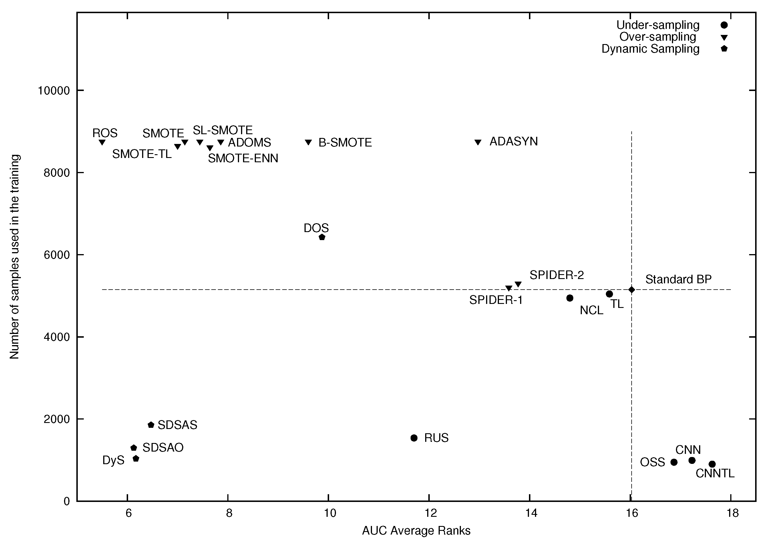
Ranks	5.500	6.129	6.171	6.471	7.000	7.143	7.443	7.643	7.857	9.600	9.871	11.700	12.971	13.586	13.771	14.800	15.586	16.029	16.871	17.229	17.629

). Second, a statistical test is presented in order to strengthen the results discussion (Figure 1). Finally, the relationship between the training dataset size and the tested methods performance is studied (Figure 2).

The results presented in Table 2 are the AUC values obtained in the classifying stage, and they are averaged values between ten folds and ten different initialization weights of the neural network (see Section 5).

In accordance with the averaged ranks shown in Table 2, all over-sampling methods and dynamic sampling approaches (SDSAO, SDSAS, DyS and DOS) can improve the standard back-propagation (BP) performance, and the worst approaches with respect to standard BP are the under-sampling techniques, except by RUS, NCL and TL, which show a better performance than the standard BP. This table also shows that only the ROS technique presents a better performance than the proposed methods. SDSAO and DyS show a slight advantage over SDSAS.

In addition, Table 2 indicates that the class Imbalance Ratio (IR) is not determinant in order to get high AUC values, for example CAY7, SAT2, SEG1, SEG5 and 92A5 datasets present high values of AUC no matter their IR; also in these datasets, most over-sampling methods and dynamic sampling approaches are very competitive.

Other datasets support this fact, i.e., IR is not critical in the classification performance, for example the SEG4 and SEG5 datasets have the same IR, but the classification performance (using the standard BP) is very different (values of AUC of 0.999 and 0.630, respectively). This confirms was was presented in other works, in that other features of the data might become a strong problem for the class imbalance [2]. For example: (i) the class overlapping or noisy data [39,42,56,57]; (ii) the small disjuncts; (iii) the lack of density and information in the training data [58]; (iv) the significance of the borderline instances [13,59] and their relationship with noisy samples; and (v) the possible differences in the data distribution for the training and testing data, also known as the dataset shift [7].

In order to strengthen the result analysis, a non-parametrical statistical and post-hoc tests are applied (see Section 5.3): Friedman and Iman–Davenport tests report that considering reduction performance distributed according to chi-square with 20 degrees of freedom, the Friedman statistic is set at 329.474, and the p-value computed by the Friedman test is $1.690$×${10}^{-10}$. However, considering reduction performance distributed according to the F-distribution with 20 and 680 degrees of freedom, the Iman and Davenport statistic is 30.233, and the p-value computed by their test is $2.588\times {10}^{-80}$. Then, the null hypothesis is rejected, i.e., the Friedman and Iman–Davenport tests indicate the existence of significant differences in the results. Due to these results, a post-hoc statistical analysis is required.

Figure 1 shows the results of the non-parametric statistical Holm and Shaffer post-hoc tests. The rows and columns constitute the studied methods; as a consequence, it represents all $C\times C$ pairwise classifier comparisons. The filled circles mean that for these particular pairwise methods (for $C_i\times C_j$; $i=1,2,...,C$ and $i\ne j$), the null hypothesis was reject by the Holm–Shaffer post-hoc tests. Therefore, the color of circles is the darkest when the p-values are close to zero; this means that the statistical difference is significant.

In accordance with Table 2 and Figure 1, most methods of over-sampling present a better classification performance than the standard BP with statistical significance. The under-sampling methods do not present a statistical difference with respect to standard BP performance, and all dynamic sampling approaches improve the standard BP performance with statistical differences.

ADASYIN, SPIDER-1 and SPIDER-2 (over-sampling methods) and RUS, NCL and TL (under-sampling methods) show the trend of improving the classification results, but they do not significantly improve the standard BP performance. Then, the OSS, CNN and CNNTL classify worse than standard BP; this notwithstanding, these approaches do not show a statistical difference with it.

SDSAO, SDSAS and DyS are statistically better than ADASYIN, SPIDER-1 and SPIDER-2 (over-sampling methods) and also than all under-sampling approaches studied in this work. With a statistical difference, the DOS performance is better than CNN, CNNTL, OSS and TL.

Table 2 shows that the trend is that ROS presents a better performance than the proposed method (SDSAO and SDSAS), and that DyS shows a slight advantage over SDSAS; however, in accordance with the Holm–Shaffer post-hoc tests, statistical difference in the classification performance does not exist among these methods (see Figure 1).

In general terms, most over-sampling methods and dynamic sampling approaches are successful methods to deal with the class imbalance problem, but with respect to the training dataset size, SDSAS, SDSAO and DyS use significantly fewer samples than the over-sampling approaches. They employed about 78% less samples than most over-sampling methods; in addition, SDSAS, SDSAO and DyS still use fewer samples than the standard BP trained with the original training dataset. They use about 60% less samples; these facts stand out in Figure 2. However, the DyS method applies the ROS in each epoch or iteration (see Section 4), whereas SDSA only applies the ROS or SMOTE one time before ANN training (see Section 2).

Figure 2 shows that the under-sampling methods employ significantly fewer samples than the rest of the techniques (except dynamic sampling approaches with respect to RUS, NCL and TL); however, their classification performance in most of the cases is worse than the standard BP (without statistical significant) or is not better (with statistical significant) than the standard BP.

On the other hand, the worst methods studied in this paper (in agreement with Table 2) are those based on the CNN technique (OSS, CNN and CNNTL), i.e., those that use a $k-NN$ rule as the basis and achieving an important size reduction of the training dataset. In contrast, NCL, which is of the $k-NN$ family, also improves the classification performance of the back-propagation; however, the dataset size reduction reached for this method is not of CNN’s magnitude; in addition, it only eliminates majority samples. The use of TL (TL and SMOTE-TL) seems to increase the classification performance, but it does not eliminate too many samples (see Figure 2), except by CNNTL, which we consider to cancel the positive effect of TL by the important training dataset reduction. SMOTE-ENN does not seem to improve the classification performance of SMOTE in spite of including a cleaning step that removes both majority and minority samples. The methods that have achieved the enhancing of the classifier performance are those that only eliminate samples from the majority class.

Furthermore, analyzing only the selective samples methods (SL-SMOTE, B-SMOTE, ADASYN, SPIDER-1 and SPIDER-2), those are the ones in which the more appropriate samples are selected to be over-sampled. It is considered that in the result presented in Figure 2, SL-SMOTE and B-SMOTE obtain the best results, whereas the advantages of ADASYN, SPIDER-1 and SPIDER-2 are not clear (RUS often outperforms these approaches, but without statistical significance; Figure 1). SL-SMOTE, B-SMOTE and the proposed method do not show statistical significance in their classification results, but the number of samples used by SDSA in the training stage is fewer than employed for SL-SMOTE and B-SMOTE (see Figure 2).

Focusing on the dynamic sampling approaches’ analysis, SDSAO presents a slight advantage in performance than DyS and SDSAS, whereas DOS does not seem to be an attractive method. However, the aim of DOS is to identify a suitable over-sampling rate, whilst reducing the processing time and storage requirements, as well as keeping or increasing the ANN performance, to obtain a trade-off between classification performance and computational cost.

SDSA and DyS improve the classification performance, including a selective process, but while DyS tries to reduce the oversampling ratio during the training (i.e., it applies the ROS method in each epoch with different class imbalance ratios; see Section 4), the SDSA only tries to use the “best samples” to train the ANN.

Dynamic sampling approaches are a very attractive way to deal with a class imbalance problem. They face two important topics: (i) improving the classification performance; and (ii) reducing the classifier computational cost.

7. Conclusions and Future Work

We propose a new Selective Dynamic Sampling Approach (SDSA) to deal with the class imbalance problem. It is attractive because it automatically selects the best samples to train the multilayer perceptron neural network with the stochastic back-propagation. The SDSA identifies the most appropriate samples (“average samples”) to train the neural network. The average samples are the most adequate samples to train the neural network; they are neither hard nor easy to learn. These are between the safe and border areas in the training space. SDSA employs a Gaussian function to give priority to the average samples during the neural network training stage.

The experimental results in this paper point out that SDSA is a successful method to deal with the class imbalance problem, and its performance is statistically equivalent to other well-known over-sampling and dynamic sampling approaches. It is statistically better than the under-sampling methods compared to this work and also than the standard back-propagation. In addition, in the neural network training stage, SDSA uses significantly fewer samples than the over-sampling methods, even than the standard back-propagation trained with the original dataset.

Future work will extend this study. The interest is: to explore the effectiveness of the SDSA in multi-class and high imbalanced problems and to find a mechanism to automatically identify the most suitable μ value for each dataset. The appropriate selection of μ value might significantly improve the proposed method. In addition, it is important to explore the possibility to use the SDSA to obtain optimal subsets to train other classifiers like support vector machines or to compare its effectiveness with the other kinds of class imbalance approaches using other learning models.

References

- Prati, R.C.; Batista, G.E.A.P.A.; Monard, M.C. Data mining with imbalanced class distributions: Concepts and methods. In Proceedings of the 4th Indian International Conference on Artificial Intelligence (IICAI 2009), Tumkur, Karnataka, India, 16–18 December 2009; pp. 359–376.
- Galar, M.; Fernández, A.; Tartas, E.B.; Sola, H.B.; Herrera, F. A review on ensembles for the class imbalance problem: Bagging-, boosting-, and hybrid-based approaches. IEEE Trans. Syst. Man Cyber. Part C 2012, 42, 463–484. [Google Scholar] [CrossRef]
- García, V.; Sánchez, J.S.; Mollineda, R.A.; Alejo, R.; Sotoca, J.M. The class imbalance problem in pattern classication and learning. In II Congreso Español de Informática; Thomson: Zaragoza, Spain, 2007; pp. 283–291. [Google Scholar]
- Wang, S.; Yao, X. Multiclass imbalance problems: Analysis and potential solutions. IEEE Trans. Syst. Man Cyber. Part B 2012, 42, 1119–1130. [Google Scholar] [CrossRef] [PubMed]
- Nanni, L.; Fantozzi, C.; Lazzarini, N. Coupling different methods for overcoming the class imbalance problem. Neurocomput 2015, 158, 48–61. [Google Scholar] [CrossRef]
- Loyola-González, O.; Martínez-Trinidad, J.F.; Carrasco-Ochoa, J.A.; García-Borroto, M. Study of the impact of resampling methods for contrast pattern based classifiers in imbalanced databases. Neurocomputing 2016, 175, 935–947. [Google Scholar] [CrossRef]
- López, V.; Fernández, A.; García, S.; Palade, V.; Herrera, F. An insight into classification with imbalanced data: Empirical results and current trends on using data intrinsic characteristics. Inf. Sci. 2013, 250, 113–141. [Google Scholar] [CrossRef]
- Chawla, N.V.; Bowyer, K.W.; Hall, L.O.; Kegelmeyer, W.P. SMOTE: Synthetic minority over-sampling technique. J. Artif. Intell. Res. 2002, 16, 321–357. [Google Scholar]
- Batista, G.E.A.P.A.; Prati, R.C.; Monard, M.C. A study of the behavior of several methods for balancing machine learning training data. SIGKDD Explor. Newsl. 2004, 6, 20–29. [Google Scholar] [CrossRef]
- He, H.; Garcia, E. Learning from imbalanced data. IEEE Trans. Knowl. Data Eng. 2009, 21, 1263–1284. [Google Scholar]
- Han, H.; Wang, W.; Mao, B. Borderline-SMOTE: A New Over-Sampling Method in Imbalanced Data Sets Learning. In Proceedings of the International Conference on Intelligent Computing (ICIC 2005), Hefei, China, 23–26 August 2005; pp. 878–887.
- Bunkhumpornpat, C.; Sinapiromsaran, K.; Lursinsap, C. Safe-level-SMOTE: Safe-level-synthetic minority over-sampling technique for handling the class imbalanced problem. In Proceedings of the 13th Pacific-Asia Conference (PAKDD 2009), Bangkok, Thailand, 27–30 April 2009; Volume 5476, pp. 475–482.
- He, H.; Bai, Y.; Garcia, E.A.; Li, S. ADASYN: Adaptive Synthetic Sampling Approach for Imbalanced Learning. In Proceedings of the 2008 IEEE International Joint Conference on Neural Networks (IJCNN 2008), Hong Kong, China, 1–8 June 2008; pp. 1322–1328.
- Stefanowski, J.; Wilk, S. Selective pre-processing of imbalanced data for improving classification performance. In Proceedings of the 10th International Conference in Data Warehousing and Knowledge Discovery (DaWaK 2008), Turin, Italy, 1–5 September 2008; pp. 283–292.
- Napierala, K.; Stefanowski, J.; Wilk, S. Learning from Imbalanced Data in Presence of Noisy and Borderline Examples. In Proceedings of the 7th International Conference on Rough Sets and Current Trends in Computing (RSCTC 2010), Warsaw, Poland, 28–30 June 2010; pp. 158–167.
- Japkowicz, N.; Stephen, S. The class imbalance problem: A systematic study. Intell. Data Anal. 2002, 6, 429–449. [Google Scholar]
- Liu, X.; Wu, J.; Zhou, Z. Exploratory undersampling for class-imbalance learning. IEEE Trans. Syst. Man Cyber. Part B 2009, 39, 539–550. [Google Scholar]
- Alejo, R.; Valdovinos, R.M.; García, V.; Pacheco-Sanchez, J.H. A hybrid method to face class overlap and class imbalance on neural networks and multi-class scenarios. Pattern Recognit. Lett. 2013, 34, 380–388. [Google Scholar] [CrossRef]
- Alejo, R.; García, V.; Pacheco-Sánchez, J.H. An efficient over-sampling approach based on mean square error back-propagation for dealing with the multi-class imbalance problem. Neural Process. Lett. 2015, 42, 603–617. [Google Scholar] [CrossRef]
- Wilson, D. Asymptotic properties of nearest neighbor rules using edited data. IEEE Trans. Syst. Man Cyber. 1972, 2, 408–420. [Google Scholar] [CrossRef]
- Kubat, M.; Matwin, S. Addressing the Curse of Imbalanced Training Sets: One-sided Selection. In Proceedings of the 14th International Conference on Machine Learning (ICML 1997), Nashville, TN, USA, 8–12 July 1997; pp. 179–186.
- Tomek, I. Two modifications of CNN. IEEE Trans. Syst. Man Cyber. 1976, 7, 679–772. [Google Scholar]
- Hart, P. The condensed nearest neighbour rule. IEEE Trans. Inf. Theory 1968, 14, 515–516. [Google Scholar] [CrossRef]
- Zhou, Z.H.; Liu, X.Y. Training cost-sensitive neural networks with methods addressing the class imbalance problem. IEEE Trans. Knowl. Data Eng. 2006, 18, 63–77. [Google Scholar] [CrossRef]
- Drummond, C.; Holte, R.C. Class Imbalance, and Cost Sensitivity: Why Under-Sampling Beats Over-Sampling. In Proceedings of the Workshop on Learning from Imbalanced Datasets II, (ICML 2003), Washington, DC, USA; 2003; pp. 1–8. Available online: http://citeseerx.ist.psu.edu/ viewdoc/summary?doi=10.1.1.132.9672 (accessed on 4 July 2016). [Google Scholar]
- He, H.; Ma, Y. Imbalanced Learning: Foundations, Algorithms, and Applications, 1st ed.; John Wiley & Sons, Inc Press: Hoboken, NJ, USA, 2013. [Google Scholar]
- Lin, M.; Tang, K.; Yao, X. Dynamic sampling approach to training neural networks for multiclass imbalance classification. IEEE Trans. Neural Netw. Learn. Syst. 2013, 24, 647–660. [Google Scholar] [PubMed]
- Wang, J.; Jean, J. Resolving multifont character confusion with neural networks. Pattern Recognit. 1993, 26, 175–187. [Google Scholar] [CrossRef]
- Ou, G.; Murphey, Y.L. Multi-class pattern classification using neural networks. Pattern Recognit. 2007, 40, 4–18. [Google Scholar] [CrossRef]
- Murphey, Y.L.; Guo, H.; Feldkamp, L.A. Neural learning from unbalanced data. Appl. Intell. 2004, 21, 117–128. [Google Scholar] [CrossRef]
- Fernández-Navarro, F.; Hervás-Martínez, C.; Antonio Gutiérrez, P. A dynamic over-sampling procedure based on sensitivity for multi-class problems. Pattern Recognit. 2011, 44, 1821–1833. [Google Scholar] [CrossRef]
- Fernández-Navarro, F.; Hervás-Martínez, C.; García-Alonso, C.R.; Torres-Jiménez, M. Determination of relative agrarian technical efficiency by a dynamic over-sampling procedure guided by minimum sensitivity. Expert Syst. Appl. 2011, 38, 12483–12490. [Google Scholar] [CrossRef]
- Chawla, N.V.; Cieslak, D.A.; Hall, L.O.; Joshi, A. Automatically countering imbalance and its empirical relationship to cost. Data Min. Knowl. Discov. 2008, 17, 225–252. [Google Scholar] [CrossRef]
- Debowski, B.; Areibi, S.; Gréwal, G.; Tempelman, J. A Dynamic Sampling Framework for Multi-Class Imbalanced Data. In Proceedings of the Machine Learning and Applications (ICMLA), 2012 11th International Conference on (ICMLA 2012), Boca Raton, FL, USA, 12–15 December 2012; pp. 113–118.
- Alejo, R.; Monroy-de-Jesus, J.; Pacheco-Sanchez, J.; Valdovinos, R.; Antonio-Velazquez, J.; Marcial-Romero, J. Analysing the Safe, Average and Border Samples on Two-Class Imbalance Problems in the Back-Propagation Domain. In Progress in Pattern Recognition, Image Analysis, Computer Vision, and Applications—CIARP 2015; Springer-Verlag: Montevideo, Uruguay, 2015; pp. 699–707. [Google Scholar]
- Lawrence, S.; Burns, I.; Back, A.; Tsoi, A.; Giles, C.L. Neural network classification and unequal prior class probabilities. Neural Netw. Tricks Trade 1998, 1524, 299–314. [Google Scholar]
- Laurikkala, J. Improving Identification of Difficult Small Classes by Balancing Class Distribution. In Proceedings of the 8th Conference on AI in Medicine in Europe: Artificial Intelligence Medicine (AIME 2001), Cascais, Portugal, 1–4 July 2001; pp. 63–66.
- Prati, R.; Batista, G.; Monard, M. Class Imbalances versus Class Overlapping: An Analysis of a Learning System Behavior. In Proceedings of the Third Mexican International Conference on Artificial Intelligence (MICAI 2004), Mexico City, Mexico, 26–30 April 2004; pp. 312–321.
- Batista, G.E.A.P.A.; Prati, R.C.; Monard, M.C. Balancing Strategies and Class Overlapping. In Proceedings of the 6th International Symposium on Intelligent Data Analysis, (IDA 2005), Madrid, Spain, 8–10 September 2005; pp. 24–35.
- Tang, Y.; Gao, J. Improved classification for problem involving overlapping patterns. IEICE Trans. 2007, 90-D, 1787–1795. [Google Scholar] [CrossRef]
- Inderjeet, M.; Zhang, I. KNN approach to unbalanced data distributions: A case study involving information extraction. In Proceedings of the International Conference on Machine Learning (ICML 2003), Workshop on Learning from Imbalanced Data Sets, Washington, DC, USA, 21 August 2003.
- Stefanowski, J. Overlapping, Rare Examples and Class Decomposition in Learning Classifiers from Imbalanced Data. In Emerging Paradigms in Machine Learning; Ramanna, S., Jain, L.C., Howlett, R.J., Eds.; Springer Berlin Heidelberg: Berlin, Germany, 2013; Volume 13, pp. 277–306. [Google Scholar]
- Duda, R.; Hart, P.; Stork, D. Pattern Classification, 2nd ed.; Wiley: New York, NY, USA, 2001. [Google Scholar]
- Fawcett, T. An introduction to ROC analysis. Pattern Recogn. Lett. 2006, 27, 861–874. [Google Scholar] [CrossRef]
- Tang, S.; Chen, S. The Generation Mechanism of Synthetic Minority Class Examples. In Proceedings of the 5th International Conference on Information Technology and Applications in Biomedicine (ITAB 2008), Shenzhen, China, 30–31 May 2008; pp. 444–447.
- Bruzzone, L.; Serpico, S. Classification of imbalanced remote-sensing data by neural networks. Pattern Recognit. Lett. 1997, 18, 1323–1328. [Google Scholar] [CrossRef]
- Lichman, M. UCI Machine Learning Repository; University of California, Irvine, School of Information and Computer Sciences: Irvine, CA, USA, 2013. [Google Scholar]
- Baumgardner, M.; Biehl, L.; Landgrebe, D. 220 Band AVIRIS Hyperspectral Image Data Set: June 12, 1992 Indian Pine Test Site 3; Purdue University Research Repository, School of Electrical and Computer Engineering, ITaP and LARS: West Lafayette, IN, USA, 2015. [Google Scholar]
- Madisch, I.; Hofmayer, S.; Fickenscher, H. Roberto Alejo; ResearchGate: San Francisco, CA, USA, 2016. [Google Scholar]
- Wilson, D.R.; Martinez, T.R. Improved heterogeneous distance functions. J. Artif. Int. Res. 1997, 6, 1–34. [Google Scholar]
- Alcalá-Fdez, J.; Fernandez, A.; Luengo, J.; Derrac, J.; García, S.; Sánchez, L.; Herrera, F. KEEL data-mining software tool: Data set repository, integration of algorithms and experimental analysis framework. J. Mult. Valued Logic Soft Comput. 2011, 17, 255–287. [Google Scholar]
- Iman, R.L.; Davenport, J.M. Approximations of the critical region of the friedman statistic. Commun. Stat. Theory Methods 1980, 9, 571–595. [Google Scholar] [CrossRef]
- Holm, S. A simple sequentially rejective multiple test procedure. Scand. J. Stat. 1979, 6, 65–70. [Google Scholar]
- Luengo, J.; García, S.; Herrera, F. A study on the use of statistical tests for experimentation with neural networks: Analysis of parametric test conditions and non-parametric tests. Expert Syst. Appl. 2009, 36, 7798–7808. [Google Scholar] [CrossRef]
- García, S.; Herrera, F. An extension on “statistical comparisons of classifiers over multiple data sets” for all pairwise comparisons. J. Mach. Learn. Res. 2008, 9, 2677–2694. [Google Scholar]
- García, V.; Mollineda, R.A.; Sánchez, J.S. On the k-NN performance in a challenging scenario of imbalance and overlapping. Pattern Anal. Appl. 2008, 11, 269–280. [Google Scholar] [CrossRef]
- Denil, M.; Trappenberg, T.P. Overlap versus Imbalance. In Proceedings of the Canadian Conference on AI, Ottawa, NO, Canada, 31 May–2 June 2010; pp. 220–231.
- Jo, T.; Japkowicz, N. Class imbalances versus small disjuncts. SIGKDD Explor. Newsl. 2004, 6, 40–49. [Google Scholar] [CrossRef]
- Ertekin, S.; Huang, J.; Bottou, L.; Giles, C. Learning on the border: Active learning in imbalanced data classification. In Proceedings of the ACM Conference on Information and Knowledge Management, Lisbon, Portugal, 6–10 November 2007.