A Model to Determinate the Influence of Probability Density Functions (PDFs) of Input Quantities in Measurements

Abstract

A method for analysing the effect of different hypotheses about the type of the input quantities distributions of a measurement model is presented here so that the developed algorithms can be simplified. As an example, a model of indirect measurements with optical coordinate measurement machine was employed to evaluate these different hypotheses. As a result of the different experiments, the assumption that the different variables of the model can be modelled as normal distributions is proved.

1. Introduction

The determination measurement’s uncertainty made with coordinates measuring machines (CMMs) is an important line of research in the field of coordinate metrology [1,2].

Although there are different papers [3,4] in which the uncertainty calculation is based on GUM approach [5], this model is impractical for most situations that appear in the field of coordinate metrology, since the GUM approach does not provide a solution to the singularities that arise, for example,

• multi-dimensional models based on the coordinates of multiple points;
• the impossibility of determining the sensitivity coefficients of some parameters when these are the result of the application of filters, adjustment algorithms, etc.;
• the existence of input variables of the model that have non-symmetric distributions;
• the nonlinearity of calculation models that force one to consider higher-order terms. Wilhelm et al. [6] conducted a comprehensive analysis of the various models for calculating.

To avoid these problems, different authors have proposed different methods. Wilhelm et al. [6] used a numerical method for calculating uncertainties associated with specific measurement tasks, due to the complexity of the measures. They analysed the concept of “virtual CMM”, which materialises a very precise mathematical model of behavior of a CMM. This model simulates data acquisition, measurement strategy, and physical behavior of the CMM. By the later use of the Monte Carlo method, it is possible to determine the measurement uncertainty. Abbe et al. [7] proposed a method for the evaluation of the uncertainty associated with measurements made by a CMM from information obtained after checking the machine using the ISO 10360-2 [8].

The Monte Carlo method [9] is the appropriate solution to estimate the uncertainty associated with measurements obtained with equipment based in coordinate metrology and allows solving problems such as:

• arbitrarily complicated models or input quantities of the model present asymmetrical probability density functions (PDF).

According to Supplements 1 and 2 to the GUM [9,10], the steps to be followed to use the Monte Carlo method are as follows:

• formulation, in which the following is defined: (1) the output quantities of model (measurand), (2) the input quantities of the model, (3) the measurement model that connects the inputs with the outputs, (4) the assignment of PDF to each input quantity;
• the propagation of the PDF assigned to the input quantities using the measurement model, obtaining the PDF of each output quantity; and
• a summary determining for each output quantity, from its PDF, their mathematical expectation, standard uncertainty, uncertainty coverage interval, and covariance matrix.

It is possible to find metrological models that provide correlated output quantities with PDF not comparable to any known. When these quantities are used in subsequent calculation measurement models, the propagation of these quantities cannot use the procedures described in Supplements 1 and 2 of the GUM. In these cases, the theory of copulas is often used [11,12,13,14], which develops functions capable of describing dependencies between variables and providing multivariate data that model correlated distributions. The use of the theory of copulas has disadvantages such as high computation times and complexity of the developed algorithms, disadvantages that in an industrial environment are critical parameters.

The aim of this paper is to analyse the effect of various hypotheses about the type of the input quantities distributions of the measurement model so that the developed algorithms can be simplified. A model of indirect measurements with optical CMMs is employed, and three hypotheses effects on the measurement results (distance between graduations on a line scale and its associated uncertainty) are studied:

• the use of the theoretical distributions, obtained in the determination of the calibration parameters of the equipment;
• the simplification of the known theoretical distributions (t-student, uniform, Weibull, etc.) that better model the behaviour of the theoretical distributions are used; and
• the simplification of the theoretical distributions with normal distributions.

For this measurement model, the input quantities studied are the parameters that assure the metrological traceability of the equipment.

2. Materials and Methods

In this section, a mathematical model is presented to characterize the vision subsystem of the CMM. With a developed calibration procedure [15], it is possible to calculate the uncertainties of the measurements made therewith [16].

2.1. Optical Coordinate Measurement Machine Model

The vision subsystem model of the optical coordinate measurement machine used in this paper is the so-called affine camera, in which the optical centre is located at an infinity point [17]. This model is used to model systems with telecentric lenses/lens systems [18], allowing for the transformation of the coordinates of a point in space (3D) called “coordinates of the world system” into the coordinates of a point of an image (2D) called “coordinates of the image system digitized”. This inverse transformation is represented in the matrix form by:

$$\begin{array}{l}{\mathbf{X}}_{hm}^{\prime }={\mathbf{Q}}^{\prime }\cdot {\mathbf{U}}_{hpi}\\ {\mathbf{X}}_{hm}^{\prime }={\left[{\mathbf{R}}^{\prime }|\mathbf{t}\right]}^{-1}\cdot {\mathbf{K}}^{-1}\cdot {\mathbf{U}}_{hpi}\end{array}\}\mathrm{with}{\mathbf{K}}^{-1}=\left(\begin{array}{ccc}1/{\alpha }_x& -s/\left({\alpha }_x\cdot {\alpha }_y\right)& -\left({\alpha }_y\cdot x_0+s\cdot y_0\right)/\left({\alpha }_x\cdot {\alpha }_y\right)\\ 0& 1/{\alpha }_y& -y_0/{\alpha }_y\\ 0& 0& 1\end{array}\right),$$

(1)

where ${\mathbf{X}}_{hm}^{\prime }={\left(x_m,y_m,1\right)}^T$ are the coordinates of a point in the world system, and ] are the pixel coordinates of the digitized image system. ${\mathbf{R}}^{\prime }$ is an orthogonal rotation matrix 3 × 3, and $\mathbf{t}$ is a translation matrix 3 × 1. With these two matrixes, the position of the camera with respect to the world system is defined. $s$ characterizes the possibility of the lack of perpendicularity between the axes, $x_0,y_0$ represent the image centre coordinates, ${\alpha }_x,{\alpha }_y$ model the camera pixels size along the X- and Y-axes, and ${\mathsf{\delta }}_{u^{\prime }},{\mathsf{\delta }}_{v^{\prime }}$ represent the geometric distortion of the coordinates $u^{\prime }$ and $v^{\prime }$:

$$\begin{array}{l}{\mathsf{\delta }}_{u^{\prime }}=\stackrel{Radial}{\overbrace{k_1\Delta u^{\prime }\left(\Delta {u^{\prime }}^2+\Delta {v^{\prime }}^2\right)+k_2\Delta u^{\prime }{\left(\Delta {u^{\prime }}^2+\Delta {v^{\prime }}^2\right)}^2}}+\stackrel{Decentering}{\overbrace{p_1\left(3\Delta {u^{\prime }}^2+\Delta {v^{\prime }}^2\right)+2p_2\Delta u^{\prime }\Delta v^{\prime }}}+\stackrel{Thinprism}{\overbrace{s_1\left(\Delta {u^{\prime }}^2+\Delta {v^{\prime }}^2\right)}}\\ {\mathsf{\delta }}_{v^{\prime }}=k_1\Delta v^{\prime }(\Delta {u^{\prime }}^2+\Delta v^2)+k_2\Delta v^{\prime }{(\Delta {u^{\prime }}^2+\Delta {v^{\prime }}^2)}^2+2p_1\Delta u^{\prime }\Delta v^{\prime }+p_2(\Delta {u^{\prime }}^2+3\Delta {v^{\prime }}^2)+s_2(\Delta {u^{\prime }}^2+\Delta {v^{\prime }}^2)\end{array},$$

(2)

where $\Delta u^{\prime }=u^{\prime }-x_0,\Delta v^{\prime }=v^{\prime }-y_0$ and $k_1,k_2,p_1,p_2,s_1,s_2$ represent the geometric distortion coefficients.

By employing a fixed frequency grid distortion target, it is possible to calibrate the instrument vision subsystem [15] so that the traceability of the measures subsequently made by the equipment is ensured. The results of the calibration of a MITUTOYO equipment, model Ultra-QV350 (measuring range (X × Y × Z): 350 mm × 350 mm × 150 mm, resolution: 0.01 μm) available in the Centro Español de Metrología (CEM) (Tres Cantos, Spain) are shown below. The distortion target images (dot diameter: 65 μm and step: 125 μm) have been obtained by using diascopic illumination at 20% of its nominal value, with a magnification of 10×, which determines a nominal pixel size of 0.89 μm. The temperature during the measurement time is kept in the range 20 ± 0.2 °C.

Table 1. Results of the calibration parameters of the optical coordinate measuring machine.

Parameter	Parameter Estimation yi	Standard Uncertainty u(yi)	Shortest 95% Coverage Interval
			Lower Limit	Upper Limit
K−1(1, 1) (mm/pixel)	9.855 × 10−4	2.5 × 10−6	9.803 × 10−4	9.912× 10−4
K−1(1, 2) (mm/pixel)	9.662 × 10−7	4.8 × 10−9	9.560 × 10−7	9.768 × 10−7
K−1(1, 3) (mm)	−0.31610	0.00099	−0.31792	−0.31434
K−1(2, 2) (mm/pixel)	−9.803 × 10−4	2.5 × 10−6	−9.856 × 10−4	−9.751 × 10−4
K−1(2, 3) (mm)	0.23576	0.00076	0.23446	0.23705
ur (pixel)	320.50	0.61	320.35	320.65
vr (pixel)	240.49	0.51	240.34	240.64
k1 (pixel−2)	0.1 × 10−8	8.1 × 10−8	−1.77 × 10−7	1.76 × 10−7
k2 (pixel−4)	0.4 × 10−13	6.2 × 10−13	−1.27 × 10−12	1.33 × 10−12
s1 (pixel−1)	−0.1 × 10−6	2.3 × 10−6	−4.5 × 10−6	4.4 × 10−6
s2 (pixel−1)	0.3 × 10−6	2.3 × 10−6	−4.1 × 10−6	4.7 × 10−6
p1 (pixel−1)	−0.4 × 10−6	6.8 × 10−6	−1.34 × 10−5	1.32 × 10−5
p2 (pixel−1)	−0.1 × 10−6	5.3 × 10−6	−1.1 × 10−6	1.0 × 10−6

shows the results of the simulations performed for a number of replications M = 10⁴ (the Monte Carlo method is used for determining the uncertainty associated with the model calibration parameters).

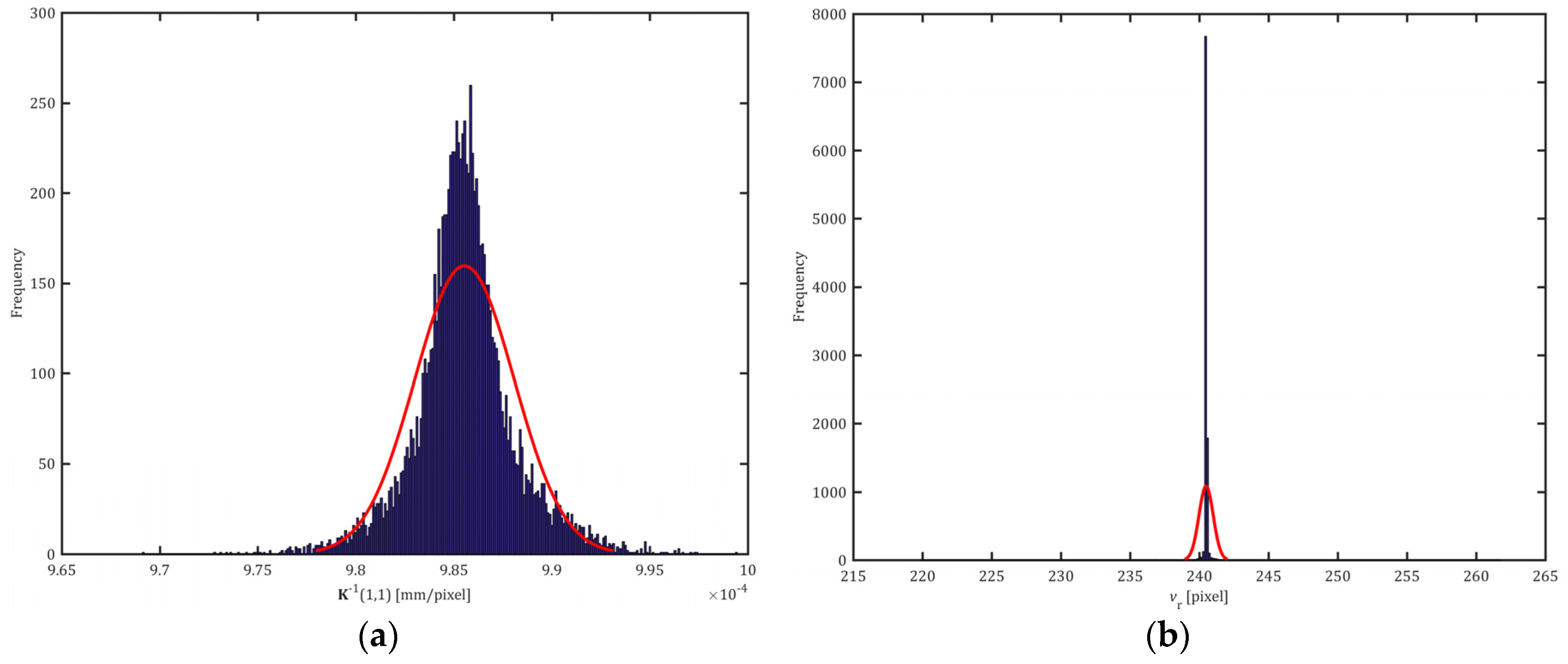
Since the above variables have common input variables, there are correlated [15]. Figure 1a,b show, as an example, some of the histograms of the output variables of the calibration model. From his analysis, and from the histograms of the variables not shown, it is possible to find that these variables could be assimilated reasonably well to the following distributions:

• t-student, with different degrees of freedom (DOF), variables, K⁻¹(1, 1), K⁻¹(1, 2), K⁻¹(1, 3), K⁻¹(2, 3), K⁻¹(2, 3), k₁, and k₂;
• normal, variables p₁, p₂, s₁, and s₂; and
• other types, variables u_r and v_r. If these distributions are analysed, it is found that 99% of their values could be assimilated reasonably well to a rectangular distribution.

The u_r and v_r variables have a high concentration of values in a relatively narrow range and very extensive distribution tails. This behaviour is due to the fact that the geometric distortion parameters obtained are practically zero, independently of the value taken by the geometric distortion centre; within limits, the corrections obtained with these parameters are virtually null.

2.2. Considerations about the Types of Distributions of the Parameters of the Vision Subsystem

As noted above, the vision subsystem parameters can be assimilated to some of the known types of distributions in a reasonably correct way. In this subsection, the effect that occurred as a result of a measurement (values of the parameter and its uncertainty) when different assumptions about the type of distribution that match the parameters of vision subsystem are made are analysed. To do this, for example, a measurement model that assesses the distance between graduations of a glass line scale and its associated uncertainty using the Monte Carlo method is implemented. The three hypotheses indicated in the introduction are considered.

For Hypotheses 2 and 3, for each vision subsystem parameter, and from the information obtained from its histogram, the mean value, standard deviation, and number of degrees of freedom (t-student distribution) are determined if necessary.

2.2.1. Procedure for Measuring a Glass Line Scale

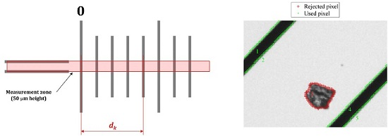
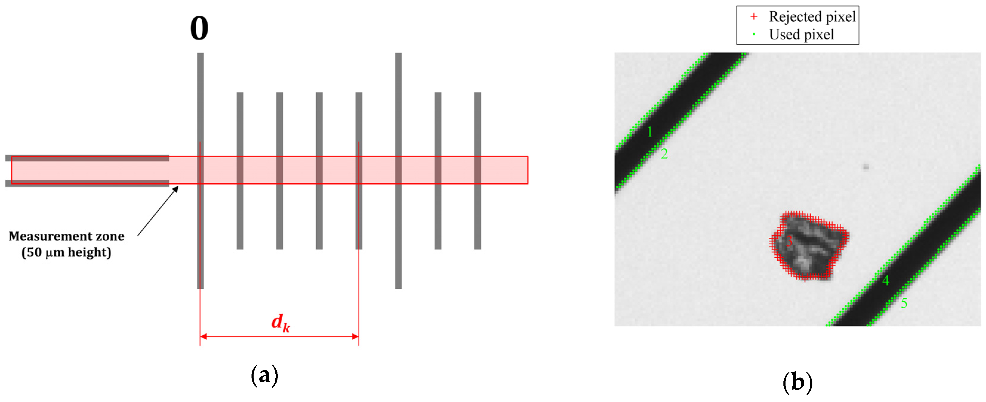
A NPL (National Physical Laboratory) glass line scale (Figure 2a), with a nominal length of 100 nm and a distance of 0.1 mm between graduations, was used. Its main purpose was to serve as a high accuracy standard for performing calibrations in the industrial area. The graduation width was about 10 μm. The scale contained two parallel horizontal lines, about 50 μm apart (Figure 2a), at the start and the end of the scale, used as an alignment axis. The coefficient of linear expansion of the scale, as indicated by the manufacturer, is: $\alpha =\left(0.5\pm 0.1\right)\times {10}^{-6}{\mathrm{K}}^{-1}$.

The glass line scale was calibrated by the CEM using a microscope-CCD camera assembly and laser interferometric system. The results up to a nominal position of 0.4 mm were as follows (

Table 2. Calibration data of the glass line scale.

Nominal Position (mm)	Measured Valued (mm)	Deviation from Nominal Position (μm)	Expanded Uncertainty (k = 2) (μm)
0	0.00000	0.00	0.08
0.1	0.10003	0.03	0.08
0.2	0.20006	0.06	0.08
0.3	0.30001	0.01	0.08
0.4	0.39999	−0.01	0.08

).

The measurands are the distances d_k between the reference centreline of the zero graduation and the centreline of the k-th graduation. The measurements were made on the section of the scale to fall between the two horizontal lines used as an alignment axis. The field of vision of the Ultra-QV350 equipment for the measurement conditions used above (magnification 10×) was 0.62 mm × 0.47 mm. Therefore, the distances between graduations of the glass line scale are measured up to the nominal position 0.4 mm so that it is possible to compare the results obtained in different positions.

This phase was divided into the following steps:

• acquisition of multiple images of the glass line scale. Ten images at intervals of 30 s were captured, with the standard in the same position, and the information obtained from the images was used in the subsequent calculation of uncertainties;
• correction and normalization of the luminance of the image [19];
• detection of the pixels that formed the edge of the glass line scale graduations (Figure 2b), employing the Canny edge detection method with “global thresholding”. Each k-th graduation of the glass line scale, with $k=0,\dots ,n_t$, has two edges, called an odd edge and even, the edges of a k-th graduation are characterized by a several number of points ($p_{k_{odd}}$, $p_{k_{even}}$), and, for each of the k graduations, the pixels of the odd edge ${\left(u_i^k,v_i^k\right)|}_{i=1}^{p_{k_{odd}}}$ and the even edge ${\left(u_j^k,v_j^k\right)|}_{j=1}^{p_{k_{even}}}$ are obtained;
• conversion of the previous coordinates (in pixels) of the edge in units of length. The above relationship is determined by the expression:

  $${\mathbf{X}}_m={\mathbf{K}}^{-1}\cdot {\mathbf{U}}_m,$$

  (3)

  where ${\mathbf{U}}_m=\left(u_m^{\prime }-{\delta }_u^{\prime },v_m^{\prime }-{\delta }_v^{\prime }\right)$ and ${\mathbf{X}}_m={\left(x_m,y_m,1\right)}^T$ are the coordinates in units of length. The components of the matrix ${\mathbf{K}}^{-1}$, the terms of geometric distortion (distortion coefficients $k_1,k_2,p_1,p_2,s_1,s_2$, and the geometric distortion centre $u_r,v_r$), were obtained in the previous calibration of the vision subsystem (Section 2.1).
• determination of the distance between graduations. Once the coordinates of the edge pixels have been processed, the distances d_k between the zero graduation and the k-th [16] are determined).

2.2.2. Model for Calculating Uncertainties

As can be deduced from the scientific literature, the Monte Carlo method is fit to determine the uncertainty of the previous values d_k distances. This method is divided into the following steps that were particularized for our mathematical model:

• Definition of output variables: the distance d_k between the zero gradation and the line k-th graduation.
• Definition of input quantities: determining the d_k distances has the following input variables: the light intensity of the pixels $I\left(i,j\right)$ of the image of the glass line scale and the results of the calibration of the vision subsystem materialized by ${\mathbf{K}}^{-1},u_r,v_r,k_1,k_2,s_1,s_2,p_1,p_2$, i.e., the inverse calibration camera matrix, the centre of geometric distortion and geometric distortion coefficients. If the results are corrected for the effect of temperature, it is necessary to employ the linear expansion coefficient $\alpha$ of the glass line scale and the temperature difference of the glass line scale $\Delta T$ with respect to the reference.
• Assignment of the PDF to the input variables: The uncertainty associated with the light intensity of the pixels is obtained according to the work of De Santo et al. [20]. The uncertainty of the variables is determined by the hypothesis considered:

  • Hypotheses 1 and 2: It can be difficult to generate random data with dependence when they have distributions that are not from a standard multivariate distribution. Indeed, some of the standard multivariate distributions can model only some limited types of dependence. In these cases, copulas are often used [21]. These functions can describe dependencies between variables and provide distributions that model correlated multivariate data. Its use allows the construction of bivariate or multivariate distribution by specifying marginal univariate distributions. For this, it is necessary to choose the type of copula so as to allow generating a correlation structure between variables. To simulate multivariate variables in this paper the following steps are followed:

    ○

    Simulation of a multivariate normal with zero mean and covariance matrix unit.

    ○

    Calculation of a multivariate normal with zero mean and covariance matrix ${\mathbf{U}}_{\mathbf{C}}$, which is the covariance matrix of the calibration results of the vision subsystem, Equation (4):

    $${\mathbf{U}}_{\mathbf{C}}=\left(\begin{array}{cccc}{u}^2\left({\mathbf{K}}^{-1}\left(1,1\right)\right)& u^2\left({\mathbf{K}}^{-1}\left(1,1\right),{\mathbf{K}}^{-1}\left(1,2\right)\right)& \cdots & u^2\left({\mathbf{K}}^{-1}\left(1,1\right),p_2\right)\\ u^2\left({\mathbf{K}}^{-1}\left(2,1\right),{\mathbf{K}}^{-1}\left(1,1\right)\right)& u^2\left({\mathbf{K}}^{-1}\left(1,2\right)\right)& \cdots & u^2\left({\mathbf{K}}^{-1}\left(1,2\right),p_2\right)\\ ⋮& ⋮& \ddots & ⋮\\ u^2\left(p_2,{\mathbf{K}}^{-1}\left(1,1\right)\right)& u^2\left(p_2,{\mathbf{K}}^{-1}\left(1,2\right)\right)& \cdots & u^2\left(p_2\right)\end{array}\right).$$

    (4)

    ○

    Prior transformation of normal uniforms, whose values are contained in the interval [0, 1].

    ○

    It is possible to obtain the variable $c_i$ from the variable using the inverse function $F^{-1}\left(u_i\right)$:

    $$c_i=F^{-1}\left(u_i\right).$$

    (5)

    In the case of Hypothesis 1, the probability distribution function $F\left(x\right)$ is estimated using a kernel density estimation (KDE) [22,23]; in the case of Hypothesis 2, the probability distribution function $F\left(x\right)$ is a known, univariate marginal distribution (normal, t-student, …).

  • Hypothesis 3: The uncertainty of the variables $\mathbf{c}=\left({\mathbf{K}}^{-1},u_r,v_r,k_1,k_2,s_1,s_2,p_1,p_2\right)$ is calculated from the covariance matrix obtained in the calibration of the vision subsystem. As noted in Section 2.1, these variables are correlated. This hypothesis assumes that the above variables have PDF equivalent to Gaussian distributions. Taking into account the recommendations of Supplement 1 to the GUM, the determination of the PDF of these variables uses the method of multivariate normal distribution [9]. Multivariate normal distribution $\mathbf{N}\left(\mathbf{c},{\mathbf{U}}_{\mathbf{C}}\right)$ is assigned to variables $\mathbf{c}$.
• Propagation: considering that the calculation model is relatively complex, the recommendation of Supplement 1 to the GUM, Section 7.2.3 [9], is taking into account. In response to this recommendation, the model is replicated a number of times equal to 10⁴.
• Summary: the statistics variable mean and standard deviation of the values obtained in the simulations shall be calculated. To calculate the coverage interval, the shortest interval method is used [24].

3. Results

Once the model for calculating the distances d_k and for estimating its associated uncertainties was defined, the measurement of the glass line scale was performed in a position approximately parallel to the $X$ axis of the machine.

The measurement was performed with the optical equipment Ultra-QV350, whose characteristics have already been defined in Section 2.1. The glass line scale images were obtained by using transmitted illumination at 20% of its nominal value with 10× magnification. The glass line scale temperature during measurement remained in the range 20 °C ± 0.1 °C. Thus, no temperature correction is applied to the distances d_k.

Table 3. Measurement results of the glass line scale in horizontal position. Hypothesis 1.

Distances	Estimate dk (mm)	Deviations to the Reference Value (nm)	Standard Uncertainty u(dk) (mm)	Shortest 95% Coverage Interval
				Lower Limit (mm)	Upper Limit (mm)
d1	0.10003	2	0.00020	0.09961	0.10047
d2	0.20006	−4	0.00038	0.19930	0.20094
d3	0.30009	−76	0.00037	0.29930	0.30083
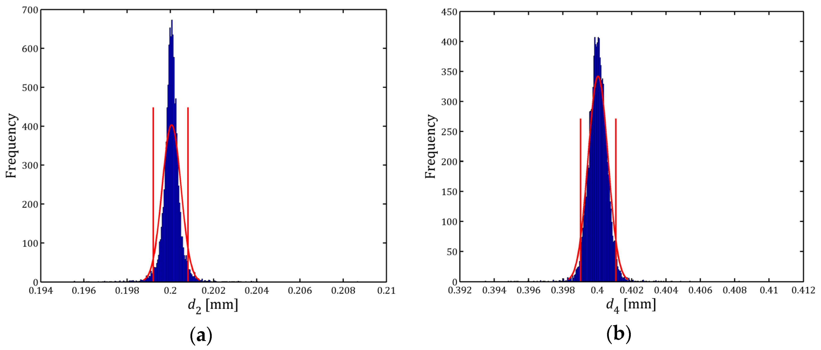
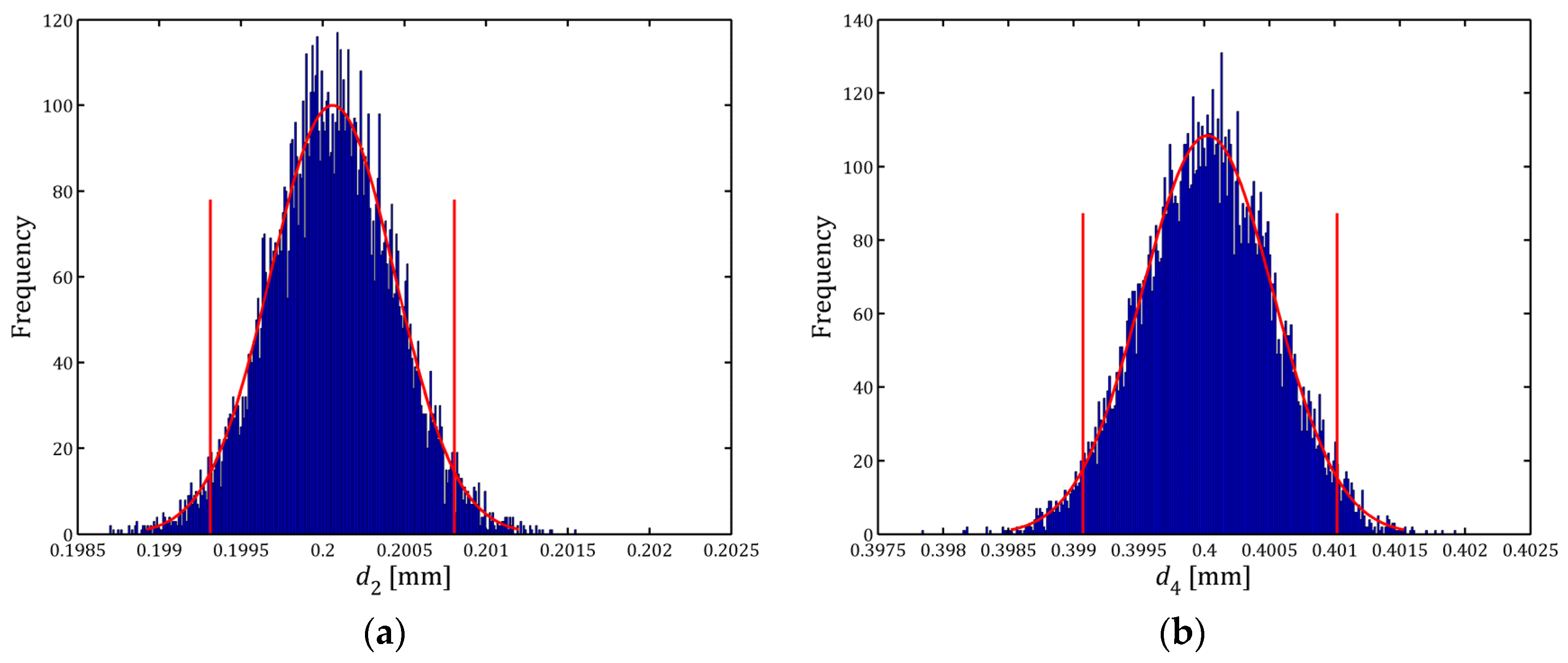
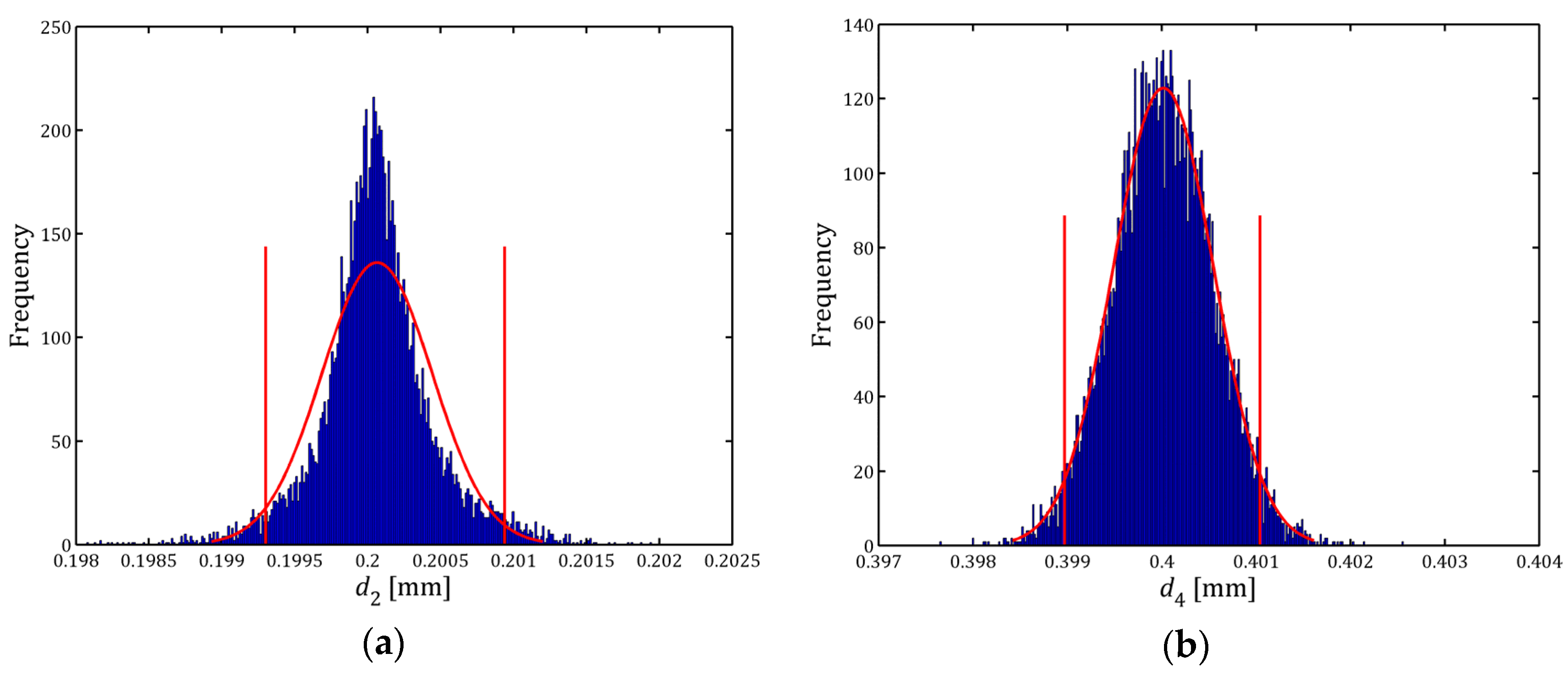
d4	0.40002	−27	0.00053	0.39897	0.40104

shows the results obtained by measuring the glass line scale considering the Hypothesis 1. Figure 3a,b show the histograms of the distances d₂ and d₄. These results obtained by developing the Hypotheses 2 and 3 are shown in

Table 4. Measurement results of the glass line scale in horizontal position. Hypothesis 2.

Distances	Estimate dk (mm)	Deviations to the Reference Value (nm)	Standard Uncertainty u(dk) (mm)	Shortest 95% Coverage Interval
				Lower Limit (mm)	Upper Limit (mm)
d1	0.10002	7	0.00023	0.09960	0.10043
d2	0.20006	4	0.00043	0.19921	0.20082
d3	0.30009	−75	0.00044	0.29935	0.30082
d4	0.40004	−49	0.00058	0.39903	0.40108

, Figure 4a,b and

Table 5. Measurement results of the glass line scale in horizontal position. Hypothesis 3.

Distances	Estimate dk (mm)	Deviations to the Reference Value (nm)	Standard Uncertainty u(dk) (mm)	Shortest 95% Coverage Interval
				Lower Limit (mm)	Upper Limit (mm)
d1	0.10002	5	0.00020	0.09962	0.10042
d2	0.20006	0	0.00038	0.19931	0.20081
d3	0.30009	−75	0.00037	0.29937	0.30080
d4	0.40002	−34	0.00050	0.39907	0.40102

, Figure 5a,b, respectively. Analyzing the results of the above tables, it is observed that variations within a single estimate of the measurand d_k obtained in the various hypotheses are between 1 nm and 22 nm, values that can be considered negligible considering that the nominal size pixel in the measurement conditions used was 0.98 μm.

By performing the same analysis for the standard uncertainty of the distances d_k, it was found that it varied between 26 nm and 74 nm. These variations were greater as distance d_k increased. When the results of Hypotheses 1 and 3 were compared, it was determined that its variation was between 1 nm and 30 nm. As in the previous case, these variations can be considered negligible.

If the histograms of Figure 3, Figure 4 and Figure 5 are compared, it is found that there are great similarities between those obtained in Hypotheses 1 and 3, that is, when histograms are equal to the theoretical distributions obtained from the calibration of the vision subsystem and when they are assimilated to normal distributions. Finally, regardless of the hypothesis considered, if the distance d_k increases, the histogram for this variable approaches a normal distribution.

4. Conclusions

In this paper, a model for evaluating the influence of the PDFs of input quantities on the output quantities of a measurement model when the measurements are obtained with an optical measuring machine is presented.

The Monte Carlo method is employed to evaluate the uncertainty of the output quantities because this method is the appropriate solution in this type of metrological problem.

When the form of the distributions of input quantities is analysed, in some cases, these do not present known distributions. To employ the Monte Carlo method to calculate the uncertainty in that case, the copula method must be used to generate random correlated data.

Three different hypotheses have been established to analyse the effect of the PDF form in the measurement results. In view of the results obtained, variations lower than 22 nm, it is assumed that the input quantities of the model can be simplified and assimilated to normal distributions.

This allows for a simplifying assumption, reduces the computation time of the programs developed for the subsequent calculation of uncertainties, and reduces the complexity of the code used for generating multivariate random variables, among other benefits. This experimental work may be applied to any model that presents correlated input variables.

References

- Kunzmann, H.; Trapet, E.; Wäldele, F. A uniform concept for calibration, acceptance test, and periodic inspection of coordinate measuring machines using reference objects. CIRP Ann. Manuf. Technol. 1990, 39, 561–564. [Google Scholar] [CrossRef]
- Schwenke, H.; Siebert, B.; Wäldele, F.; Kunzmann, H. Assessment of uncertainties in dimensional metrology by Monte Carlo simulation: Proposal of a modular and visual software. CIRP Ann. Manuf. Technol. 2000, 49, 395–398. [Google Scholar] [CrossRef]
- Wladyslaw, M.S.; Plowucha, W. Analytical estimation of coordinate measurement uncertainty. Measurement 2012, 45, 2299–2308. [Google Scholar]
- Ali, S.H.R.; Buajarern, J. New method and uncertainty estimation for plate dimensions and surface measurements. J. Phys. Conf. Ser. 2014, 483. [Google Scholar] [CrossRef]
- BIPM; IEC; IFCC; ILAC; ISO; IUPAC; IUPAP; OIML. Guide to the Expression of Uncertainty in Measurement; JCGM 100:2008 GUM 1995 with Minor Corrections. Available online: http://www.bipm.org/utils/common/documents/jcgm/JCGM_100_2008_E.pdf (accessed on 23 June 2016).
- Wilhelm, R.; Hocken, R.; Schwenke, H. Task specific uncertainty in coordinate measurement. CIRP Ann. Manuf. Technol. 2001, 50, 553–563. [Google Scholar] [CrossRef]
- Abbe, M.; Nara, M.M.; Takamasu, K. Uncertainty evaluation of CMM by modeling with spatial constraint. In Proceedings of the 9th International Symposium on Measurement and Quality Control (ISMQC), Chennai, India, 21–24 November 2007; pp. 121–125.
- ISO 10360-2: 2009. Geometrical Product Specifications (GPS)—Acceptance and Reverification Tests for Coordinate Measuring Machines (CMM)—Part 2: CMMs Used for Measuring Linear Dimensions; International Standards Organization: Geneva, Switzerland, 2009. [Google Scholar]
- BIPM; IEC; IFCC; ILAC; ISO; IUPAC; IUPAP; OIML. Supplement 1 to the ‘Guide to the Expression of Uncertainty in Measurement’—Propagation of Distributions Using a Monte Carlo method. JCGM 101:2008. Available online: http://www.bipm.org/utils/common/documents/jcgm/JCGM_101_2008_E.pdf (accessed on 23 June 2016).
- BIPM; IEC; IFCC; ILAC; ISO; IUPAC; IUPAP; OIML. Supplement 2 to the ‘Guide to the Expression of Uncertainty in Measurement’—Extension to Any Number of Output Quantities. JCGM 102:2011. Available online: http://www.bipm.org/utils/common/documents/jcgm/JCGM_102_2011_E.pdf (accessed on 23 June 2016).
- Possolo, A. Copulas for uncertainty analysis. Metrologia 2010, 47. [Google Scholar] [CrossRef]
- Papaefthymiou, G.; Kurowicka, G. Using Copulas for Modeling Stochastic Dependence in Power System Uncertainty Analysis. IEEE Trans. Power Syst. 2009, 24, 40–49. [Google Scholar] [CrossRef]
- Moazami, S.; Golian, S.; Kavianpour, M.R.; Hong, Y. Uncertainty analysis of bias from satellite rainfall estimates using copula method. Atmos. Res. 2014, 137, 145–166. [Google Scholar] [CrossRef]
- Possolo, A.; Elster, C. Evaluating the uncertainty of input quantities in measurement models. Metrologia 2014, 51. [Google Scholar] [CrossRef]
- Caja, J.; Gómez, E.; Maresca, P. Optical measuring equipments. Part I: Calibration model and uncertainty estimation. Precis. Eng. J. Int. Soc. Precis. Eng. Nanotechnol. 2015, 40, 298–304. [Google Scholar] [CrossRef]
- Caja, J.; Gómez, E.; Maresca, P. Optical measuring equipments. Part II: Measurement traceability and experimental study. Precis. Eng. J. Int. Soc. Precis. Eng. Nanotechnol. 2015, 40, 305–308. [Google Scholar] [CrossRef]
- Hartley, R.; Zisserman, A. Multiple View Geometry in Computer Vision, 2nd ed.; Cambridge University Press: Cambridge, UK, 2004. [Google Scholar]
- Li, D.; Tian, J. An accurate calibration method for a camera with telecentric lenses. Opt. Lasers Eng. 2013, 51, 538–541. [Google Scholar] [CrossRef]
- Santo, M.D.; Liguori, C.; Paolillo, A.; Pietrosanto, C. Standard uncertainty evaluation in image-based measurements. Measurement 2004, 36, 347–358. [Google Scholar] [CrossRef]
- Santo, M.D.; Liguori, C.; Pietrosanto, A. Uncertainty characterization in image based measurements: A preliminary discussion. IEEE Trans. Instrum. Meas. 2000, 49, 1101–1107. [Google Scholar] [CrossRef]
- Nelsen, R.B. An Introduction to Copulas, 2nd ed.; Springer-Verlag: New York, NY, USA, 2006. [Google Scholar]
- Sheather, S.J.; Jones, M.C. A Reliable Data-Based Bandwidth Selection Method for Kernel Density Estimation. J. R. Stat. Soc. Ser. B Methodol. 1991, 53, 683–690. [Google Scholar]
- Willink, R. Uncertainty analysis by moments for asymmetric variables. Metrologia 2006, 43. [Google Scholar] [CrossRef]
- Fotowicz, P. An analytical method for calculating a coverage interval. Metrologia 2006, 43, 42–45. [Google Scholar] [CrossRef]
© 2016 by the authors; licensee MDPI, Basel, Switzerland. This article is an open access article distributed under the terms and conditions of the Creative Commons Attribution (CC-BY) license (http://creativecommons.org/licenses/by/4.0/).