Article

A Pretreatment Method for the Velocity of DVL Based on the Motion Constraint for the Integrated SINS/DVL

1
School of Instrument Science & Engineering, Southeast University, No. 2, Sipailou, Nanjing 210096, China
2
Key Laboratory of Micro-inertial Instrument and Advanced Navigation Technology, Ministry of Education, No. 2, Sipailou, Nanjing 210096, China
*
Author to whom correspondence should be addressed.
These authors contributed equally to this work.
Appl. Sci. 2016, 6(3), 79; https://doi.org/10.3390/app6030079
Submission received: 21 October 2015 / Revised: 26 February 2016 / Accepted: 1 March 2016 / Published: 11 March 2016

Abstract

:
It is difficult for autonomous underwater vehicles (AUVs) to obtain accurate aided position information in many locations because of underwater conditions. The velocity accuracy from the Doppler velocity log (DVL) is a key element in deciding the AUV position accuracy when the integration system of Strapdown Inertial Navigation System/DVL/Magnetic Compass/Press Sensor (SINS/DVL/MCP/PS) is adopted. However, random noise and sudden noise in DVL caused by sound scattering, fishing populations, and seafloor gullies introduce level attitude errors and accumulate as position error. To restrain random noise, a velocity tracing method is designed based on the constant velocity model and the assumption of slow motion of AUV. To address sudden noise, a fault diagnosis method based on the χ 2 rule is introduced to judge sudden changes from innovation. When a sudden change occurs, the time update of the velocity from the tracing model is used for data fusion instead of the velocity from DVL. Simulation test results indicate that with this velocity tracing algorithm, random noise in the DVL can be effectively restrained. The level attitude accuracy and the level position accuracy are also improved with the time update of the velocity when the sudden change occurs.

1. Introduction

Autonomous underwater vehicles (AUVs) are widely used for both military and civilian purposes, such as submarine resource investigation, surveying, and detection [1,2,3]. Because of the specificity of submarine conditions, especially the strong attenuation of the GNSS signals in the water of global navigation satellite system (GNSS), satellite-based technology is ineffective underwater; thus, high accurate positioning technology underwater becomes one of the key and difficult technologies of AUV [1,2,3]. The strapdown inertial navigation system (SINS) is self-directed, highly robust, has a high update frequency of enriched navigation data and small size, and is successfully used for AUV navigation [1,2,3,4]. Due to the inherent errors in sensors and initial alignment errors, the errors of SINS navigation data are accumulated with time [3]. The error accumulation problem is the inherent and is a bottleneck problem of SINS based on integrated operation.
To solve the error accumulation problem of SINS, external aided positioning data should be introduced to correct SINS regularly. The most commonly used submarine positioning methods include GNSS, long/short baseline acoustic system (L/SBL), and geophysical field database (such as terrain and gravity). To access the GNSS data, the AUV should rise or sail near to the water surface because radio signals are easily damped and not feasible in deep water. At the same time, LBL and the geophysical database rely on the presence of a known transponder network or a known terrain, that is to say, there are preconditions to using these methods [5,6,7,8].
Recently, with the development of acoustic velocity measuring technology, the measuring distance and accuracy of Doppler velocity log (DVL) have been improved significantly. Taking RDI WHN-600 as an example, the error of the velocity is within 0.2% and the maximum operating distance is 90 m with a working frequency of 600 kHz, whereas the error is 0.5% and the distance is 500–525 m with 150 kHz [5,6]. Currently, DVL is widely used for AUV navigation and the integrated SINS/DVL has become a standard device for AUV [1,2,3,5,6].
When the integrated system of SINS/DVL is used in AUV, the level position accuracies, including the latitude and longitude, are mainly determined by the accuracy of the DVL velocity due to the lack of external position reference. Whereas the accuracy of DVL is fixed, the accuracy of SINS/DVL is mainly determined by the data fusion algorithm [1,2,3]. Numerous fusion algorithms for SINS/DVL are available in the literature, including non-linear filtering, online error calibration, and DVL-aided alignment [9,10,11,12,13,14,15]. In contrast to the above problems, this paper focuses on how to address the random and sudden noise in DVL.
The velocity-matching mode is used in SINS/DVL [4,5,6,10,12]. With velocity matching, random noise in the level attitudes and velocities is introduced by the random noise in the DVL measurement, and sudden errors in level attitudes are generated by the sudden change in DVL. Errors in specific forces are generated, which will be accumulated as velocity and position errors with integrated operation [4]. To solve the random noise and sudden changes in DVL, in this paper, a constant velocity motion model is introduced to trace the measured velocity of the DVL based on the assumption of gentle motion of the AUV underwater, and a fault diagnosis method based on χ 2 rules is introduced to judge the sudden change from innovations [16,17,18,19]. When sudden changes occur, the time update of velocity from tracing model is used to perform data fusion instead of the velocity from DVL.
In the integration of SINS/DVL, due to the low observability of yaw misalignment caused by velocity matching, a magnetic compass (MCP) is always used to provide aided yaw information. Meanwhile, for the divergence of the height and upward velocity of the SINS and the low accuracy of the upward velocity from DVL, a press sensor (PS) is used to provide aided height (or depth) information. In addition to SINS/DVL integration, MCP and PS are also used to construct an integrated navigation system to fulfill a long time and long distance navigation mission.
The rest of this paper is organized as follows. The integrated navigation system structure is described in Section 2. The disciplines and error propagation models for each subsystem are also introduced. Then, the data fusion algorithm for an integrated navigation system is described in Section 3. In Section 4, the negative effect of DVL error is analyzed, and the velocity tracing model is given based on the analysis on the characteristics of AUV motion. In Section 5, the tracing problem for the DVL velocity is simulated, and the results indicate that with this pretreatment of the DVL velocity, the navigation accuracy can be improved. Finally, some conclusions are drawn in Section 6.

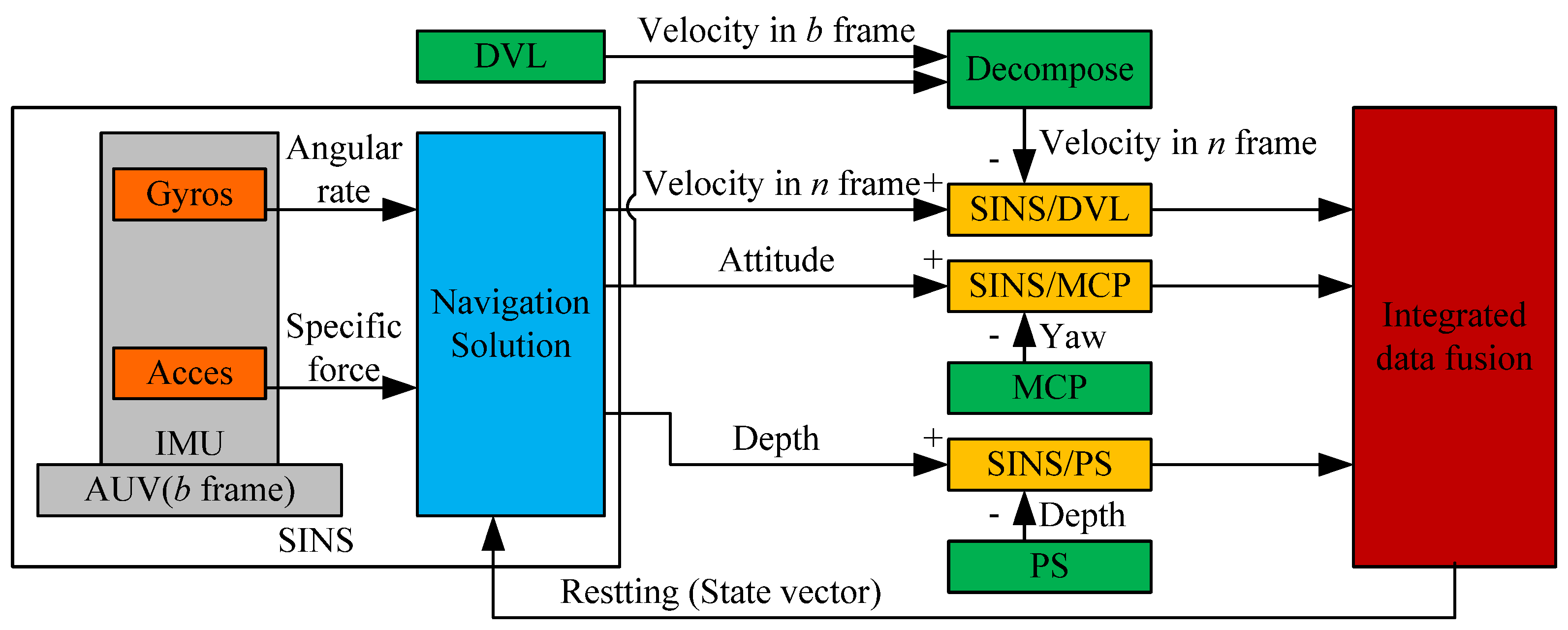
2. Integrated Navigation System of SINS/DVL/MCP/PS

The integrated navigation system of SINS/DVL/MCP/PS shown in Figure 1 is adopted, which is similar to the navigation scheme presented in [5,6]. Considering the difficulty of obtaining the aided level position in underwater conditions, the position reference system in [5,6] is abandoned.
In Figure 1, the SINS constitutes the basic navigation system providing the attitude, velocity and position of AUV through integration of the angular rate and acceleration measured by gyroscopes and accelerometers, whereas DVL, MCP and PS provide velocity, yaw, and height for data fusion with a federated Kalman filter [5,6]. In the data fusion process, subsystems constructed by SINS and aided systems, including SINS/DVL, SINS/MCP, and SINS/PS, are first built with standard Kalman liking filters (such as Kalman Filter, Extended Kalman Filter, and Unscented Kalman Filter) used for data fusion; then, a federated Kalman filter is used to fuse the information from all subsystems to obtain the estimation [5,6].
The navigation solutions of the SINS and data fusion are two independent and parallel processes. As shown in Figure 1, these two processes are connected with a closed feedback mode. The estimations from the federated Kalman filter are used to reset the navigation parameters and to compensate for sensor errors. Error propagation models are the basis of data fusion. In the following subsections, error models for each subsystem will be introduced.

2.1. Error Propagation Model of SINS

The SINS is composed of an inertial measurement unit (IMU) and a navigation solution unit. In the IMU, three gyroscopes and accelerometers are orthogonally installed to measure the vehicle’s motion with six degrees of freedom. As a self-depended navigation method, SINS can provide attitude, velocity, and position with solutions for the angular rates and accelerations. The differential equations describing the solution process are as follows [4]:
C ˙ b n = C b n ( ω n b b × )
V ˙ n = C b n f b ( 2 ω i e n + ω i e n ) × V n + g n
L ˙ = V N n R M + h , λ ˙ = V N n sec L R N + h , h ˙ = V U n
where ω n b b = ω i b b ( C b n ) T ( ω i e n + ω e n n ) , ω e n n = [ V N n / ( R M + h ) V E n / ( R N + h ) V E n tan L / ( R N + h ) ] T . Superscripts (or subscripts) of n , b , i and e denote navigation, body, inertial and earth frames. The symbol A B C D denotes the projected motion vector of A from frame C to frame B in frame D , i.e., ω e n n denotes the velocity rated from the navigation frame to the earth frame in the navigation frame, C b n is the attitude matrix in the SINS describing the converting relationship from frame b to frame n , and V n = [ V E n V N n V U n ] T is the velocity vector of SINS in navigation frame. L , λ , and h denote the latitude, longitude, and height of SINS. R M and R N denote the radius of Earth in meridian and prime, respectively, whereas the symbol “ × ” denotes the skew symmetric matrix of the vector. In the SINS solution, Equations (1)–(3) should be discretized to update the calculation; more details can be found in [4].
Errors in attitude, velocity, and position are generated because of inherent sensor errors, including the biases of gyroscopes and accelerometers, and initial alignment errors, such as initial misalignment errors and navigation solution algorithm errors. The error propagation process of the SINS can be described as follows [4]:
ϕ ˙ = ϕ × ω i n n + δ ω i n n C b n ε b
δ V ˙ n = ϕ × f b + ( 2 δ ω i e n + δ ω i e n ) × V n + ( 2 ω i e n + ω i e n ) × δ V n + C b n b
δ L ˙ = δ V N n R M + h δ h V N n ( R M + h ) 2 , δ λ ˙ = δ V N n sec L R N + h δ h V N n sec L ( R N + h ) 2 + δ L V N n sec L tan L R N + h , δ h ˙ = δ V U n
where ϕ denotes the misalignment defined as the Euler angle describing the rotation relationship between the calculated navigation frame n ' and the ideal navigation frame n , δ V n , δ L , δ λ , and δ h denote the errors of the velocity, latitude, longitude and height, δ A , such as δ ω i e n , denotes the error of vector A , and ε b and b are the errors of gyroscopes and accelerometers projected in frame b . In Equations (4)–(6), the error of gravity is ignored.
The precision of inertial sensors is the key element to determine the precision of the SINS; generally, the errors in the sensors can be classified as constant and random errors. Selecting a suitable model to describe inertial sensors is a challenge; different sensors have different characteristics. In engineering, the one-order (or high-order) Markov process and white noise are used to propagate random noise. In this paper, the main target is to pretreat the DVL measurement, and white Gaussian noise is selected to simplify the discussion. Thus, the error propagation models of gyroscopes and accelerometers can be constructed as follows:
ε ˙ b = 0 , ˙ b = 0
The statistical characteristics of the random noise of gyroscopes and accelerometers, denoted as w g b and w a b , are as follows:
w g b ~ ( 0 ,   Q g b ) , w a b ~ ( 0 , Q a b )
where Q g b and Q a b are the variance matrices of white noise corresponding to w g b and w a b , respectively.

2.2. Error Propagation Model of DVL

In DVL, Doppler effects are used to measure the velocity. With four acoustic beams in fixed directions, named the Janus configuration, three velocities along the body frame axes can be measured. Generally, the accuracy of the upward velocity is lower than those in the level direction. The precision of DVL is affected by several factors, such as installation error, scale factor error, and frequency measurement errors. For the purposes of this paper, the constant errors are assumed to be well-compensated. The random error in the DVL caused by acoustic scattering and environment changing is the focus. In engineering, random error can be described by a one-order Markov process or white Gaussian noise. To simply the analysis, white Gaussian noise is selected, and the statistical characteristics are as follows [5,6]:
w DVL b ~ ( 0 , R DVL b ) ,
where w DVL b is the random errors in DVL, and R DVL b is the variance matrix of white noise corresponding to w DVL b .

2.3. Error Propagation Models of MCP and PS

MCP and PS are important aided navigation systems. To shorten the length of this paper, the characteristics of the MCP and PS measurements are not given in detail but can be found in [5,6,12]. Similarly to DVL, white Gaussian noise is used to describe the measuring noise in MCP and PS as follows:
w MCP ~ ( 0 , R MCP )
δ h ˙ PS = 0 ,   w PS ~ ( 0 , R PS ) ,
where w MCP is the random errors in MPC, and R MCP is the variance of the white noise corresponding to w MCP . w PS is the random noise in PS, and R PS is the variance of the white noise corresponding to w PS .
In AUV, SINS, DVL, MPC, and PS are discrete systems and operate independently; thus, the measurement noise of each is assumed to be non-related.

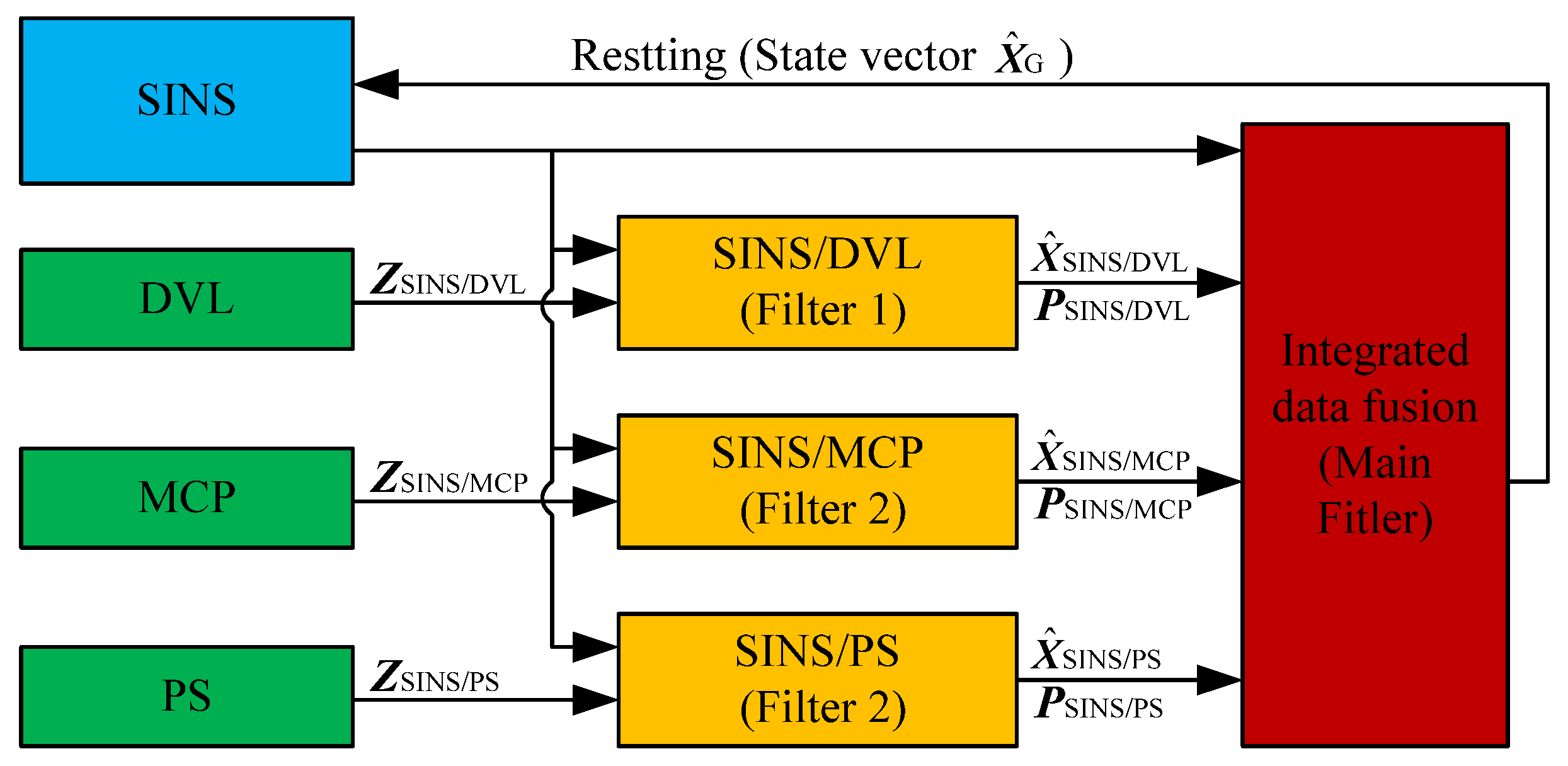
3. Data Fusion in the Integration of SINS/DVL/MCP/PS

3.1. Data Fusion with the Subsystems

Considering the computational complexity of the data fusion process, the federated Kalman filter is used for data fusion. As shown in Figure 1, the subsystems are constructed with SINS and other aided systems, i.e., DVL, MCP, and PS. The standard Kalman filter is selected as the data fusion method for each subsystem. The algorithm of the Kalman filter and the state equations and measurement equation of subsystems are introduced as follows.

3.1.1. Standard Kalman Filter

The discrete random linear model without controlling terms can be described as follows:
{ X k = Φ k , k 1 X k 1 + W k Z k = H k X k 1 + V k ,
where X is the state vector, Z is the measurement vector, Φ is the system dynamic model (or state transition matrix), H is the measurement matrix. W ~ ( 0 , Q ) denotes the system noise with the variance of Q , V ~ ( 0 , R ) denotes the measurement noise with variance of R , and k denotes the k t h time-step.
When the system noise and measurement noise are non-related and Q 0 and R > 0 , the vector X ^ k can be estimated by the standard Kalman filter. The equations in the standard Kalman filter are as follows:
{ X ^ k , k 1 = Φ k , k 1 X ^ k 1 P k , k 1 = Φ k , k 1 P k 1 Φ k , k 1 T + Q k 1 K k = P k , k 1 H k T [ H k , k 1 P k , k 1 H k , k 1 T + R k ] 1 X ^ k = X ^ k , k 1 + K k [ Z k H k X ^ k , k 1 ] P k = [ I K k H k ] P k , k 1 [ I K k H k ] T + K k R k K k T
where X ^ is the estimation of X , P is the matrix of state variance, X ^ k , k 1 and P k , k 1 are the one-step predictions at time k with X ^ k 1 and P k 1 at time k 1 , K denotes the gain matrix, and I is a unit matrix with corresponding dimensions.

3.1.2. System and Measurement Equations of SINS/DVL

Assuming the constant error in DVL is completely compensated, misalignment angles, velocity and position errors, and gyroscope and accelerometer biases in SINS are chosen as components of the state vector X SINS/DVL :
X = [ δ V E n δ V N n δ V U n ϕ E ϕ N ϕ U δ L δ λ δ h ε x b ε y b ε z b x b y b z b ] T
When the elements of the state vector are fixed, the state transition matrix defined in Equation (12) can be acquired by the discretization of Equations (3)–(6), and the variance matrix Q can be set according to the sensor precision.
Take the velocity from DVL as the aided velocity, and the measurement vector can be constructed as:
Z SINS/DVL = [ V E n V DVL E n V N n V DVL N n V U n V DVL U n ] T
where V DVL E ~ U n denotes the projected velocity in frame n , which can be calculated as V DVL n = C b n V DVL b , and V DVL b denotes the measured DVL velocity in frame b .
According to the relationship between the measurement and state vector, H SINS/DVL ( t ) can be expressed as:
H SINS/DVL = [ 1 0 0 0 1 0 0 3 × 12 0 0 1 ]
The variance matrix R corresponding to measurement noise V in Equation (12) is set according to the random noise in V DVL n . From the projection process V DVL n = C b n V DVL b , it can be observed that there is cross-noise between C b n and V DVL b . In this paper, the enlarged variance of V is used to include the crossed noise, and more details to address this noise can be found in [12]. In the following sections, this noise is not considered, and SINS and DVL are assumed to be independent.

3.1.3. System and Measurement Equations of SINS/MCP and SINS/PS

Similarly, the system and measurement equations of SINS/MCP and SINS/PS can be constructed. In Equation (14), only the error in SINS is considered, so the system equations of SINS/MCP and SINS/PS are the same with that of SINS/DVL. The measurement vector of SINS/MCP and H SINS/MCP ( t ) can be constructed as:
Z SINS/MCP = ψ ψ MCP
H SINS/DVL = [ 0 1 × 5 1 0 1 × 9 ] ,
where ψ and ψ MCP denote the yaw in SINS and MCP, respectively. The variance matrix R corresponding to measurement noise V in Equation (12) is set according to the random noise in ψ MCP .
The measurement vector of SINS/PS and H SINS/PS ( t ) can be constructed as:
Z SINS/PS = h h PS
H SINS/DVL = [ 0 1 × 8 1 0 1 × 6 ] ,
where h and hPS are the heights in SINS and PS, respectively. The variance matrix R corresponding to measurement noise V in Equation (12) is set according to the random noise in hPS.

3.2. Data Fusion of SINS/DVL/MCP/PS

The estimated vectors X ^ SINS/DVL , X ^ SINS/MCP , and X ^ SINS/PS from the subsystems should be further fused in the federated Kalman filter, named the main filter, to acquire the optimal estimation. As shown in Figure 2, the federated filter with non-feedback to the subsystems is chosen. The main advantage of this structure lies in its low complexity and non-cross interaction between each subsystem.
With no feedback, the main filter performs data fusion without filtering. The algorithm running in the main filter is as follows:
{ P G = ( P SINS/DVL 1 + P SINS/MCP 1 + P SINS/PS 1 ) 1 X ^ G = P G ( P SINS/DVL 1 X ^ SINS/DVL + P SINS/MCP 1 X ^ SINS/MCP + P SINS/PS 1 X ^ SINS/PS )
The above equation requires that all subsystems are independent and that there is cross coupling. The DVL, MPC, and PS in this paper are run independently and satisfy this requirement.

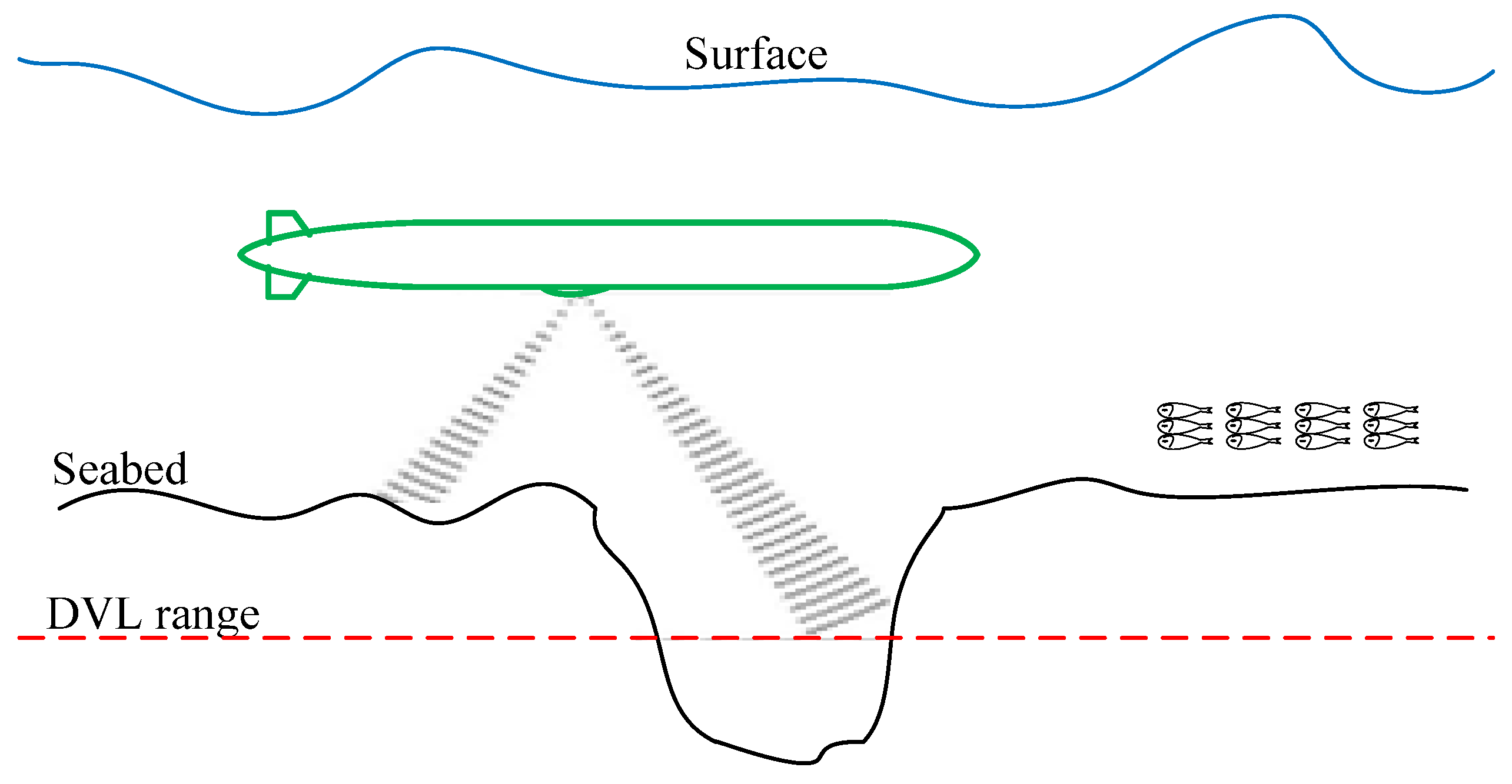
4. Velocity Tracing Method for DVL Based on Motion Constraint

4.1. Analysis of the Relationship between the DVL Error and SINS Navigation Accuracy

With the above integrated navigation scheme, the errors in DVL, MCP, and PS introduce estimation errors in both the subsystems and the main filter, and navigation errors of the estimation are fed-back to SINS. In SINS/DVL/MCP/PS, because there is no external position-aided information, the accuracy of the level position is mainly determined by the accuracy of DVL.
In the integration of SINS/DVL, constant error in the aided velocity leads to constant error in the measurement vector through velocity matching. Moreover, the constant error in measurement vector leads to estimation error in the velocity, i.e., error in the SINS velocity. Then, the velocity error generates constant errors in misalignment and constant errors in attitude, which cause analytical errors in the specific force. With integration, errors in the specific force cause velocity and position errors. Due to the lack of aided position information, the position errors cannot be corrected.
Due to the significantly negative role of the constant errors in DVL, they should be effectively compensated in engineering. For the specific working conditions shown in Figure 3, taking the work-mode against the seafloor of DVL as an example, the following scenarios exist: (1) when the AUV sails across the seafloor gully, the velocity from the DVL suddenly changes to zero because the distance between the AUV and the seafloor exceeds the measuring range; (2) when the AUV sails across a fish population, the velocity from DVL suddenly changes from the relative velocity between the AUV and the seafloor to that between the AUV and the fish. Unfortunately, these sudden changes cannot be predicted. As explained above, the sudden changes in DVL velocity cause position errors that cannot be corrected. How to judge and compensate these sudden changes plays an important role in increasing the positioning accuracy. In engineering, these sudden changes are considered as faults, and fault diagnosis based on χ 2 rules can be adopted to evaluate them. However, when these sudden changes are identified and isolated, finding a substitution to data fusion becomes a new problem.
Similarly to constant errors, random errors in DVL have also attracted significant attention. Several self-adaptive filters have been presented from the aspects of error parameter modeling. Optimal estimation can be obtained only when the model and statistical parameters are consistent with actual ones [3,4,5,6,12,14]. However, how to restrain random noise with mathematical methods has received little attention. The random noise in DVL can be treated as a constant error lasting for a short time, which also introduces errors in the SINS attitude, velocity, and position. Due to the short duration, the random noise with positive and negative changes is smoothed with integrated operation; thus, the position error caused by random noise is small. However, the errors in attitude and velocity caused by DVL random noise cannot be smoothed. Therefore, the variances of the SINS attitude and the velocity errors are partly determined by the variances of the DVL random noise. When SINS/DVL acts as an attitude reference system, random noise in DVL decreases its accuracy.
Similar analysis can be performed with MCP and PS. For the purposes of this paper, the constant errors in MCP and PS are assumed to be fully compensated, the random errors are well modeled, and the static parameters are effective.
To solve the problems of sudden changes and random noise in DVL, a velocity tracing algorithm is proposed based on the moving characteristics of the AUV in the next section.

4.2. Velocity Tracing Algorithm for DVL Based on AUV Motion Constraints
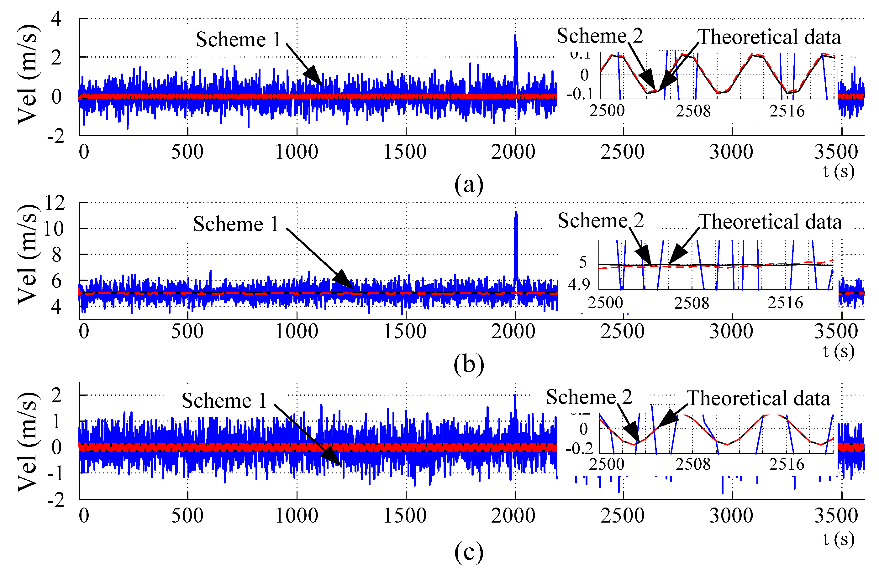
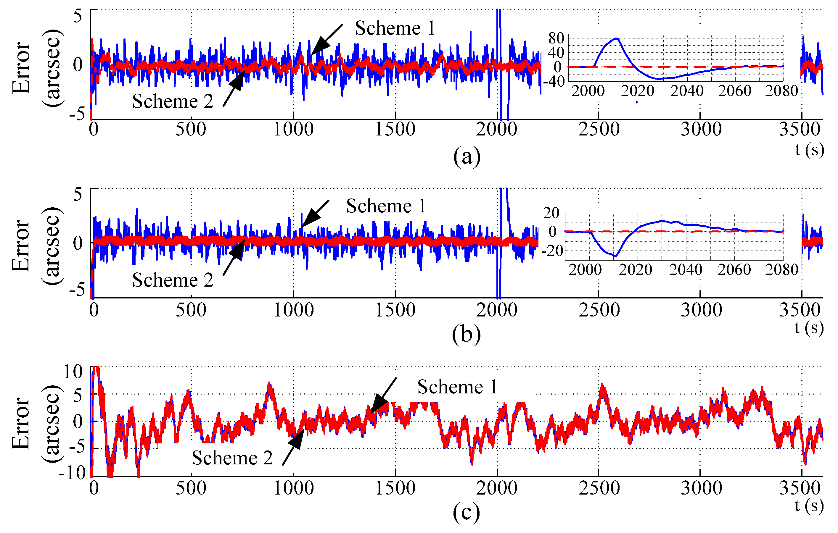
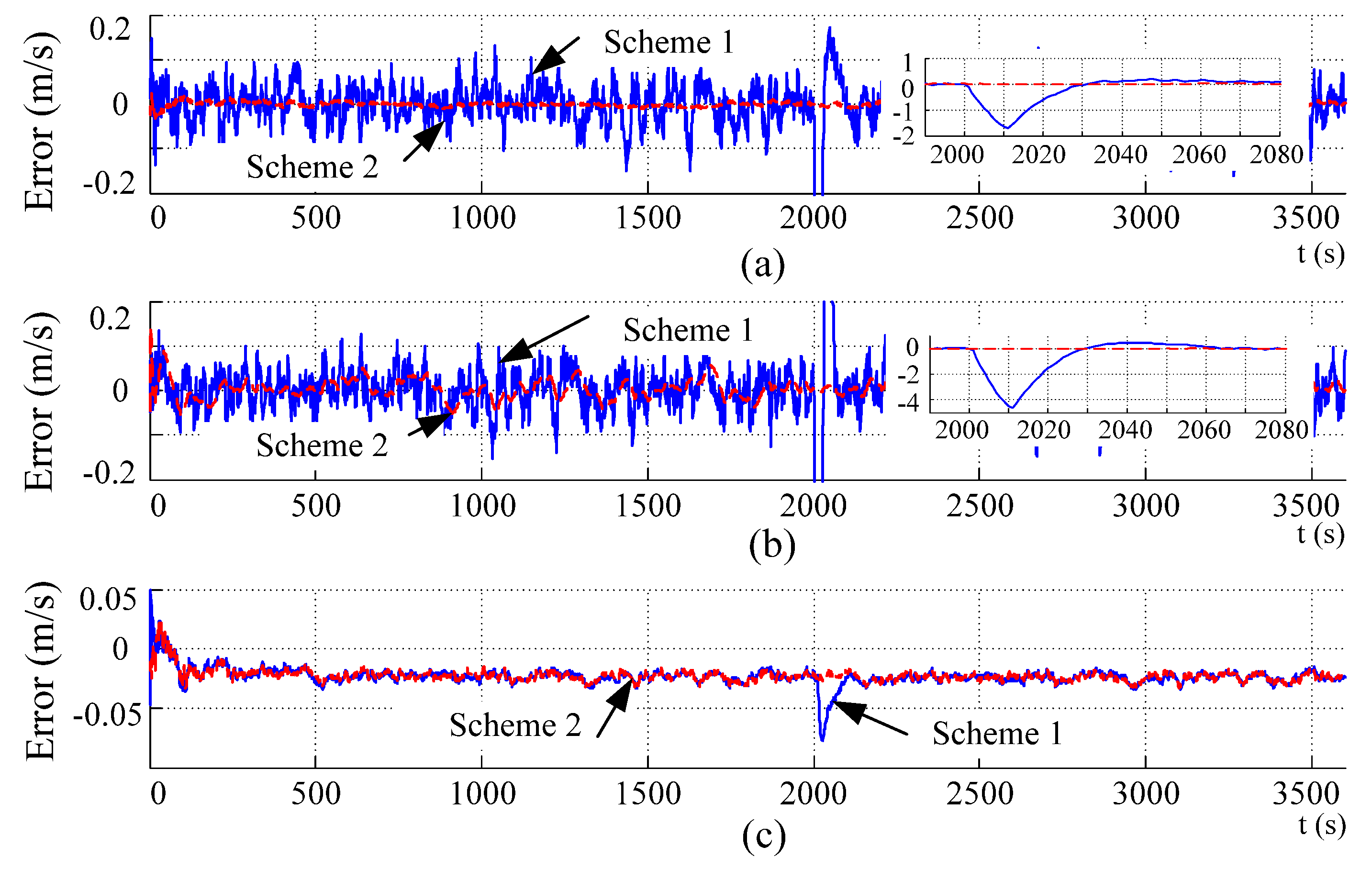
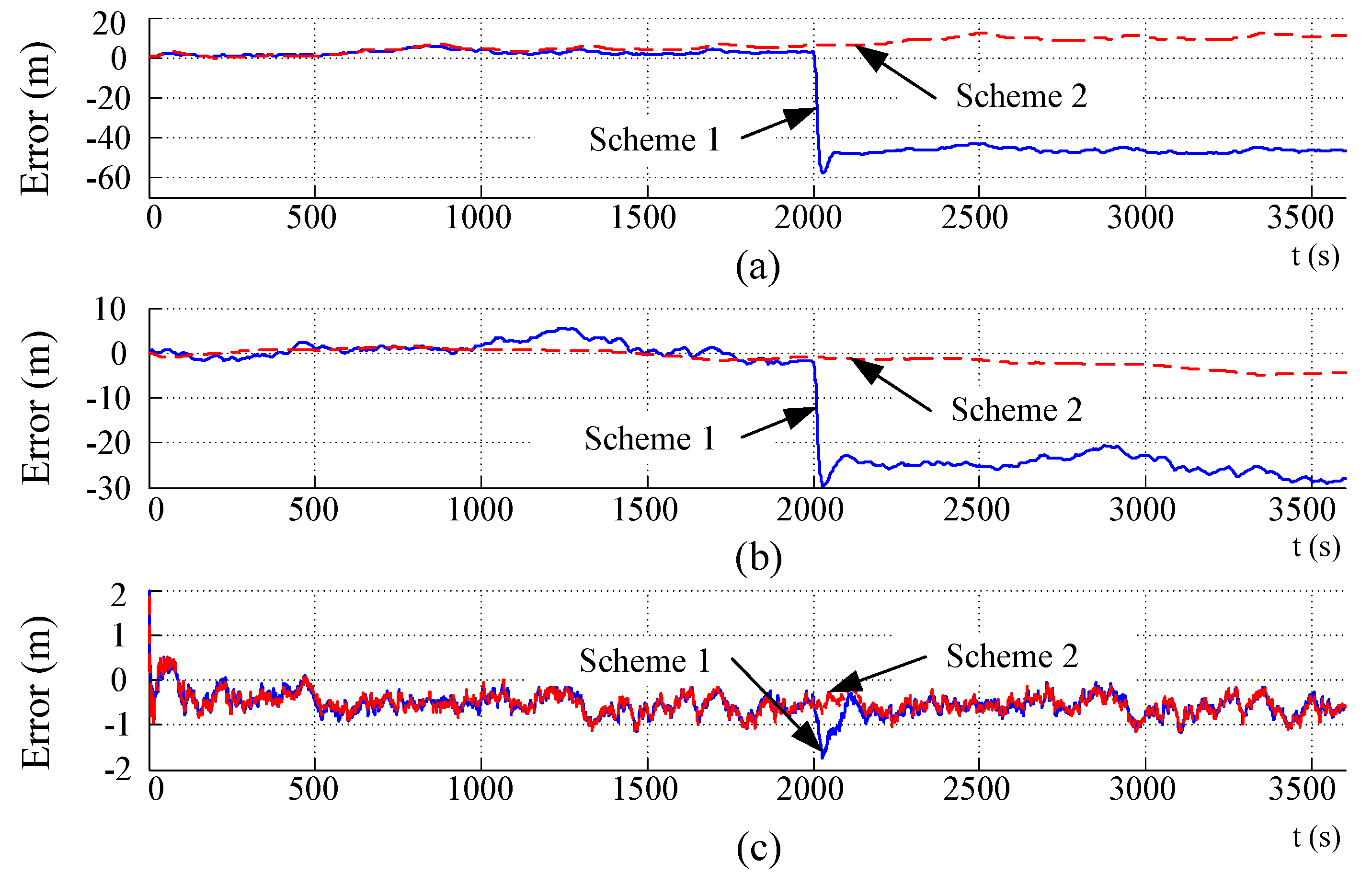
When the AUV sails, it is driven by an engine, steering, and currents. It is difficult to construct an accurate model describing the motion relationship between the input and output. However, for AUVs conducting long time and distance sailing tasks, they prefer to sail at an economic velocity. Therefore, the driving force from the engine and steering is constant. If the circle wave is ignored and only linear current is considered, the velocity and (or) acceleration of the AUV along the body frame can be addressed as a constant or slowly changing value [17].
To simplify the analysis, the current is assumed to be zero. In this condition, the velocity along the forward direction of the AUV is a fixed value. When the “right-forward-up” frame is adopted as the body frame, the velocity along the y-axis can be considered as a constant value and acceleration as zero. In this condition, the velocity V b y and acceleration a b y can be selected as the state vector, and the measured velocity from the DVL can be used as the measurement vector. Then, the system and measurement equations can be constructed as:
{ X ˙ b y ( t ) = [ V b y a b y ] = [ 0 1 0 0 ] X b y ( t ) + [ 1 0 0 1 ] w b y ( t ) Z b y ( t ) = [ 1 0 ] X b y ( t ) + v b y ( t ) ,
where Z b y = ( v DVL b x ) 2 + ( v DVL b y ) 2 + ( v DVL b z ) 2 , w b y = [ w v b y w a b y ] T denotes the disturbance caused by the excitation of the wave, which can be considered as system noise, and v b y is considered measurement noise. After discretization of Equation (22), the time and measurement can be updated with Equation (13), and the instant DVL velocity V ^ b y is estimated. When the line current is considered, the velocity along both the x-axis and z-axis should be managed with the same model of Equation (22).
When the estimation V ^ b y along the y-axis of the AUV is obtained, the velocity of the AUV in the body frame can be constructed as V ^ DVL b = [ 0 V ^ b y 0 ] T . After this velocity vector is projected into the navigation frame with the SINS attitude matrix, C b n V ^ DVL b can be used for data fusion in the SINS/DVL.
Based on the above model, the random noise is effectively restrained, which will be proved in the next section. When there is a short, sudden change in DVL velocity, the time update velocity can be used as the substitute velocity to perform data fusion. Then, how to judge this sudden change becomes a problem.
Fault diagnosis with χ 2 rules is a common method to detect sudden changes in engineering [16]. In this method, the measurement at time k 1 is assumed without a sudden change, and the prediction X ^ k , k 1 with state vector at k 1 is without error. If the measurement at k has only random noise, the innovation (also defined as the residual error) is a white noise sequence. However, when the measurement Z k at k has a sudden change, the innovation undergoes a large change. When the change is above a particular threshold, it can be deduced that a sudden change occurs.
Defining the innovation as
r k = Z k H k X ^ k , k 1
and the covariance matrix as
A k = H k P k , k 1 H k T + R k ,
the detected parameter can be defined as:
γ k = r k T A k 1 r k .
When threshold D is selected, the decision rules can be constructed as:
{ γ k D  with a sudden change γ k < D  without a sudden change .

5. Simulations

5.1. Simulation Setting

The sensors used in SINS are assumed to have mid-precision. The constant bias and random noise of gyroscopes and accelerometers are illustrated in Table 1. The AUV sails along the y-axis with a velocity of 5 m/s. Driven by interference of the current, the AUV sails with a swinging motion, and the swinging motion has the function A  sin ( 2 π f t + η 0 ) + θ 0 , in which A and f are the amplitude and frequency of the swinging and η 0 and θ 0 are the initial phase and swinging center. The swinging parameters are shown in Table 2. The initial longitude, latitude, and height of the AUV are set as 118° E, 32° N, and −20 m.
Based on the ideal motion, the theoretical sensor outputs can be obtained by back-stepping of the navigation solution. When the sensor errors are added into the theoretical outputs, the real sensor data can be simulated. To assess the navigation accuracy, the ideal motion can be used as a reference. During the simulation, the update frequency of the sensor data and navigation solution are both 100 Hz.
In the simulation, without considering the constant error, the random noise in DVL, MCP, and PS is assumed as white noise with variances of 0.5 m/s, 2°, and 0.5 m. When these errors are added to the ideal motion, the real outputs of the DVL, MCP, and PS can be simulated. During simulation, the update frequency of the DVL, MPC, and PS is set to 10 Hz.
Straight line trajectory is chosen in the simulation, and the velocity is set as above because this trajectory has no canceling effect on error growth [5,6]. To simulate the sudden velocity change in DVL, velocities of 2 m/s, 5 m/s, and 1 m/s are added to the real output of the DVL along three directions during the period 2000–2010 s.
When the initial parameters for SINS are set, the integrated navigation, including the initial alignment, is executed. Among those initial parameters, the initial velocity and position are set without any error, whereas the attitude has misalignment angles of 0.2°, 0.2°, and 1.0° in the pitch, roll and yaw.
The parameters for the Kalman filter in Section 2 are set as:
X SINS/DVL0 = [ 0 0 0 0 0 0 0 0 0 0 0 0 0 0 0 ] T ,
P SINS/DVL 0 = diag [ ( 0.5 m / s ) 2 ( 0.5 m / s ) 2 ( 0.5 m / s ) 2 ( 5 ) 2 ( 5 ) 2 ( 15 ) 2 ( 300 / R e ) 2 ( 300 / R e ) 2 ( 1 m ) 2 ( 500 ug ) 2 ( 500 ug ) 2 ( 500 ug ) 2 ( 5 / h ) 2 ( 5 / h ) 2 ( 5 / h ) 2 ] ,
Q SINS/DVL = diag [ ( 50 ug ) 2 ( 50 ug ) 2 ( 50 ug ) 2 ( 0.01 ) 2 ( 0.01 ) 2 ( 0.01 ) 2 ( 30 / R e ) 2 ( 30 / R e ) 2 ( 0.1 m ) 2 0 0 0 0 0 0 ] ,
X SINS/DVL0 = X SINS/MCP0 = X SINS/PS0 , P SINS/DVL 0 = P SINS/MCP 0 = P SINS/PS 0 , Q SINS/DVL = Q SINS/MCP = Q SINS/PS ,
R SINS/DVL = diag [ ( 0.5 m / s ) 2 ( 0.5 m / s ) 2 ( 0.5 m / s ) 2 ] , R SINS/MCP = ( 0.5 ) 2  and  R SINS/PS = ( 0.5 m ) 2
Two schemes are compared. In Scheme 1, the data fusion method introduced in Section 2 is simulated. In Scheme 2, the data fusion method with the velocity tracing method in Section 3, with the detecting threshold set at 50, is adopted.
In Scheme 2, the parameters for the velocity tracing filter are set as X b y 0 = [ V b y 0 ] T , P b y 0 = [ 1000 1000 ] T , Q b y 0 = [ 0.0005 0.005 ] T and R b y 0 = ( 0.5 3 ) 2 .

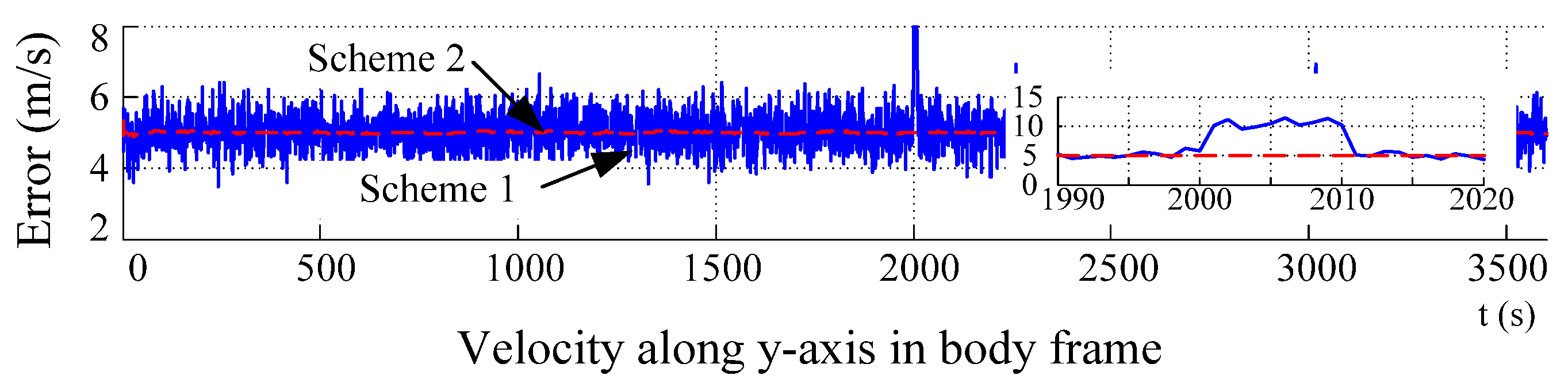
5.2. Simulation Results and Analysis

The simulation runs for 3600 s, and the simulation results are given in Figure 4, Figure 5, Figure 6, Figure 7 and Figure 8. The velocity and traced velocity in the body frame along the y-axis and in the navigation frame are listed in Figure 4 and Figure 5, where solid lines and dashed lines denote the velocity before and after tracing, respectively, named Schemes 1 and 2. The statistic results for Schemes 1 and 2 are shown in Table 3. In Scheme 1, the data during 2000–2010 s are omitted because of the sudden change in velocity.
The curves in Figure 4 and the statistic results in Table 3 indicate that before and after tracing, the means of both velocities are similar, but the standard variances are significantly different, which means the random noise in the DVL velocity can be significantly restrained by the velocity tracing algorithm. The curves in Figure 5 indicate that when the traced velocity in the body frame is projected into the navigation frame, the random noise can be restrained. The partial enlarged drawing in Figure 4 and Figure 5 indicates that the traced velocities almost coincide with the theoretical ones. When a sudden change occurs, the fault diagnosis algorithm based on χ 2 rules can judge this sudden change immediately, and the time update of the tracing algorithm can be used as a substitute output of the DVL.
The navigation results of the integrated SINS/DVL/MCP/PS are shown in Figure 6, Figure 7 and Figure 8, where the attitude, velocity and position errors are identified, and solid lines and dashed lines denote Schemes 1 and 2, respectively. To acquire a direct display, the unit of the position error in the level position is transformed from degrees to meters. The curves in Figure 6c coincide with each other because the same yaw from MCP is used in both schemes.
The curves in Figure 6, Figure 7 and Figure 8 indicate that when there is a sudden change in the DVL velocity, with Scheme 1, sudden changes in attitude, velocity, and position are introduced. When the sudden change in velocity is eliminated, the sudden change in attitude and velocity can be restrained gradually, whereas the sudden change in the level position cannot be restrained because it is an open loop. The height error is restrained because the calculation for height is a closed loop. With the height from the PS, the sudden change in height caused by a sudden change in DVL velocity is corrected.
The curves in Figure 6, Figure 7 and Figure 8 further indicate that with Scheme 2, the amplitude of the attitude and velocity errors is decreased, and the sudden change in DVL velocity does not generate a sudden change in attitude, velocity and position, as in Scheme 1. The statistical results are shown in Table 4. Considering the adjustment period when a sudden change disappears, only the data in the period of 500–2000 s are used. The statistics in Table 4 show that the tracing algorithm can effectively restrain the random noise in the DVL velocity.
From the above analysis, it can be concluded that with the velocity tracing method, the random noise in the DVL velocity can be effectively restrained, and the accuracy of the attitude and velocity can be increased. With the substituted velocity from the velocity tracing method, the position accuracy can be improved when a sudden change in the DVL velocity occurs.

6. Conclusions

An integrated navigation scheme of SINS/DVL/MCP/PS for AUVs is presented in this paper, and the error propagation models and data fusion schemes are studied. The analysis indicates that under submarine conditions, the position accuracy is mainly determined by the accuracy of the DVL because of the shortness of the external reference level position information. The negative effects caused by the random noise and sudden change in the measurements of the DVL velocity are investigated. The analysis shows the random noise in the DVL causes random oscillation in the level attitude and velocity and decreases their accuracy. In addition, the sudden change caused by seafloor gullies and fish populations generate sudden changes in the level position that cannot be corrected and significantly decrease the accuracy of the level position.
To solve these problems, the characteristics of the AUV when sailing for a long time and a long distance are analyzed, and it is concluded that the AUV always sails at a constant and economic velocity or changes slowly. The acceleration along the axes of the body frame can be assumed to be as zero or nearly zero. Then, a velocity tracing algorithm based on a constant velocity motion model is designed to restrain the random noise in the velocity from the DVL, in which the velocity disturbance caused by the wave is considered as system noise. Then, the fault diagnosis based on χ 2 rules is introduced to judge the sudden change, and the time update velocity in the model is used to perform data fusion instead of the velocity from the DVL when the sudden change occurs.
Simulation results based on the straight line trajectory indicate that with this velocity tracing algorithm, the random noise and sudden change in DVL can be effectively restrained, the standard variance in the level attitude and velocity can be decreased, and the level position accuracy can be ensured.

Acknowledgments

This work has been supported in part by the National Natural Science Foundation of China (61273056, 61101163) and the Nature Science Foundation of Jiangsu Province of China (No. BK2012739, BK20130628).

Author Contributions

All authors discussed the contents of the manuscript. Xi-Xiang Liu contributed to the research idea and the framework of this study. Li-Ye Zhao, Xian-Jun Liu, and Lei Wang performed the experimental work. Li-Ye Zhao wrote the manuscript. Yan-Hua Zhu revised and polished the manuscript.

Conflicts of Interest

The authors declare no conflicts of interest.

References

  1. Paull, L.; Saeedi, S.; Seto, M.; Li, H. AUV navigation and localization: A review. IEEE J. Ocean. Eng. 2014, 39, 131–149. [Google Scholar] [CrossRef]
  2. Brown, H.; Kim, A.; Eustice, R.M. An overview of autonomous underwater vehicle research and testbed at PeRL. Mar. Technol. Soc. J. 2009, 43, 37–47. [Google Scholar] [CrossRef]
  3. Stutters, L.; Liu, H.; Tiltman, C.; Brown, D.J. Navigation technologies for autonomous underwater vehicles. IEEE Trans. Syst. Man Cybern. 2008, 38, 581–589. [Google Scholar] [CrossRef]
  4. Titterton, D.H.; Weston, J.L. Strapdown Inertial Navigation Technology, 2nd ed.; Lavenham Press Ltd.: London, UK, 2004; pp. 263–274. [Google Scholar]
  5. Jalving, B.; Gade, K.; Hagen, O.K. A toolbox of aiding techniques for the HUGIN AUV integrated inertial navigation system. Model. Identif. Control 2004, 25, 173–190. [Google Scholar] [CrossRef]
  6. Jalving, B.; Gade, K.; Hagen, O.K. DVL velocity aiding in the HUGIN 1000 integrated inertial navigation system. Model. Identif. Control 2004, 25, 223–235. [Google Scholar] [CrossRef]
  7. Lee, P.M.; Jun, B.H. Pseudo long base line navigation algorithm for underwater vehicles with inertial sensors and two acoustic range measurements. Ocean Eng. 2007, 34, 416–425. [Google Scholar] [CrossRef]
  8. Lee, P.M.; Jun, B.H.; Kim, K.; Lee, J.; Aoki, T.; Hyakudome, T. Simulation of an inertial acoustic navigation system with range aiding for an autonomous underwater vehicle. IEEE J. Ocean Eng. 2007, 32, 327–345. [Google Scholar] [CrossRef]
  9. Geng, Y.R.; Martins, R.; Sousa, J. Accuracy analysis of DVL/IMU/Magnetometer integrated navigation system using different IMUs in AUV. In Proceedings of the 2010 8th IEEE International Conference on Control and Automation, Xiamen, China, 9–11 June 2010; pp. 516–512.
  10. Lv, Z.P.; Tang, K.H.; Wu, M.P. Online estimation of DVL misalignment angle in SINS/DVL integrated navigation system. In Proceedings of the Tenth International Conference on Electronic Measurement & Instruments, Chengdu, China, 16–19 August 2011; pp. 336–339.
  11. Kinsey, J.C.; Whitcomb, L.L. In situ alignment calibration of attitude and doppler sensors for precision underwater vehicle navigation: Theory and experiment. IEEE J. Ocean Eng. 2007, 32, 286–299. [Google Scholar] [CrossRef]
  12. Liu, X.; Xu, X.; Liu, Y.; Wang, L. Kalman filter for cross-noise in the integration of SINS and DVL. Math. Probl. Eng. 2014, 2014. [Google Scholar] [CrossRef]
  13. Ben, Y.Y.; Zhu, Z.J.; Li, Q.; Wu, X. Aided fine alignment for marine SINS. In Proceedings of the 2011 IEEE International Conference on Mechatronics and Automation, Beijing, China, 7–10 August 2011; pp. 1630–1635.
  14. Li, W.; Wang, J.; Lu, L.; Wu, W. A novel scheme for DVL-aided SINS in-motion alignment using UKF techniques. Sensors 2013, 13, 1046–1063. [Google Scholar] [CrossRef] [PubMed]
  15. Tang, K.H.; Wang, J.L.; Li, W.L.; Wu, W.Q. A novel INS and Doppler sensors calibration method for long range underwater vehicle navigation. Sensor 2013, 13, 14583–14600. [Google Scholar] [CrossRef] [PubMed]
  16. Xu, X.; Li, P.; Liu, J. A fault-tolerant filtering algorithm for SINS/DVL/MCP integrated navigation system. Math. Probl. Eng. 2015, 2015. [Google Scholar] [CrossRef]
  17. Øyvind, H.; Oddvar, H. Model-aided INS with sea current estimation for robust underwater navigation. IEEE Ocean. Eng. 2011, 36, 316–337. [Google Scholar]
  18. Xu, W.M.; Liu, Y.C. Algorithm of multi-rate integrating multiple model for underwater target tracking. J. Electron. Inf. Technol. 2008, 30, 581–584. [Google Scholar] [CrossRef]
  19. Xu, W.M.; Liu, Y.C.; Yin, X.D. Method for underwater target tracking based on integrating multiple model. Geomat. Inf. Sci. Wuhan Univ. 2007, 32, 782–785. [Google Scholar]
Figure 1. Integrated navigation scheme of Strapdown Inertial Navigation System/Doppler Velocity Log/Magnetic Compass/Press Sensor (SINS/DVL/MCP/PS).
Applsci 06 00079 g001
Figure 2. Federated data fusion of SINS/DVL/MCP/PS.
Applsci 06 00079 g002
Figure 3. Sudden changes in the measurement of the DVL velocity.
Applsci 06 00079 g003
Figure 4. DVL velocity in the body frame.
Applsci 06 00079 g004
Figure 5. DVL velocity in the navigation frame: (a) East velocity; (b) North velocity; (c) Up velocity.
Applsci 06 00079 g005
Figure 6. Curves of the attitude errors: (a) Pitch; (b) Roll; (c) Yaw.
Applsci 06 00079 g006
Figure 7. Curves of the velocity errors: (a) East velocity; (b) North velocity; (c) Up velocity.
Applsci 06 00079 g007
Figure 8. Curves of the position errors: (a) Latitude; (b) Longitude; (c) Height.
Applsci 06 00079 g008
Table 1. Sensor errors.
AxesGyro Bias (°/h)Acce Bias (ug)
ConstantRandom (White Noise)ConstantRandom (White Noise)
x-axis0.010.015050
y-axis0.010.015050
z-axis0.010.015050
Table 2. Swinging parameters.
ParametersPitchRollYaw
Amplitude (°)1.51.51.0
Cycle (s)87.56
Initial Phase (°)000
Swinging center (°)000
Table 3. Statistical results of the Doppler Velocity Log (DVL) velocity (m/s).
Statistical ItemsVelocity along the y-axisEast VelocityNorth VelocityUpward Velocity
Sch. 1Sch. 2IdealSch. 1Sch. 2IdealSch. 1Sch. 2IdealSch. 1Sch. 2Ideal
Mean5.00025.003350.0005005.00095.00055.00080.000400
Std0.49750.022000.49960.06170.06180.50010.00200.02200.51530.09260.0925
Table 4. Statistic results of the navigation errors.
Statistical ItemsPitchRollYawEast VelocityEast VelocityEast VelocityHeight
Scheme 1Mean−0.22080.0935−0.345000.0015−0.0012−0.4873
Std1.04161.08353.93270.04060.04180.00730.2589
Scheme 2Mean−0.22320.1092−0.350700.0020−0.0015−0.4907
Std0.67730.58854.07190.00560.02310.00610.2540

