Integrating Textural and Spectral Features to Classify Silicate-Bearing Rocks Using Landsat 8 Data

Abstract

Texture as a measure of spatial features has been useful as supplementary information to improve image classification in many areas of research fields. This study focuses on assessing the ability of different textural vectors and their combinations to aid spectral features in the classification of silicate rocks. Texture images were calculated from Landsat 8 imagery using a fractal dimension method. Different combinations of texture images, fused with all seven spectral bands, were examined using the Jeffries–Matusita (J–M) distance to select the optimal input feature vectors for image classification. Then, a support vector machine (SVM) fusing textural and spectral features was applied for image classification. The results showed that the fused SVM classifier achieved an overall classification accuracy of 83.73%. Compared to the conventional classification method, which is based only on spectral features, the accuracy achieved by the fused SVM classifier is noticeably improved, especially for granite and quartzose rock, which shows an increase of 38.84% and 7.03%, respectively. We conclude that the integration of textural and spectral features is promising for lithological classification when an appropriate method is selected to derive texture images and an effective technique is applied to select the optimal feature vectors for image classification.

1. Introduction

Numerous studies have demonstrated the ability to exploit the spectral features of minerals and rocks from the reflected solar spectra for lithological mapping and mineral exploration. Based on the spectral features, from visible to near-infrared (VNIR) wavelengths, some iron-bearing minerals, such as goethite and hematite, have been found in prior research to be relatively easy to distinguish [1,2]. Because of the fundamental vibrations of Al–OH, Mg–OH, and ${{\mathrm{CO}}_3}^{2-}$ bonds in shortwave infrared (SWIR) wavelengths, many alteration minerals such as carbonates, sulfates, hydroxides, and oxides have been successfully identified and mapped using remote sensing methods [1,2,3,4]. In thermal infrared (TIR) wavelengths, igneous rocks with relatively high SiO₂ contents have diagnostic emission spectral features due to the vibration of the Si–O bond, based on which, some rock indices have been constructed, such as the sulfuric acid rock index and the carbonate rock index [5,6,7]. Spectral-feature-based approaches for lithological identification mainly focus on the conversion and enhancement of spectral features, such as principal component analysis (PCA), spectral angle mapping (SAM), band ratio (BR), relative absorption band depth (RBD), false color composite (FCC), matched-filtering, and combinations of these methods [8,9,10].

However, there are still numerous limitations for lithological identification merely based on spectral features from VNIR to SWIR wavelengths. It is common for different surface objects, as well as homogeneous objects, to have similar spectral features, and many objects do not have prominent diagnostic spectral features. For example, it is difficult to precisely identify serpentinite and granite using only spectral features, as they are often intermingled with other rocks [11]. In terms of TIR data, the spectrum is generally dominated by temperature, which results in TIR radiance containing both temperature and emissivity information. The algorithms to separate temperature and emissivity are generally complex and problematic because of the nonlinearity in the relative contributions of temperature and emissivity effects [12,13,14]. The extracted emissivity products have a relatively high uncertainty and low contrast, which may subdue spectral features and limit the discrimination accuracy [15,16]. A rock index is generally sensitive to a specific rock or mineral and is not enough to identify other rocks [4,6]. Further, the application of spectral features is less successful for lithological mapping in vegetated terrain, as the bedrock is often partially or completely occluded by vegetation [17,18]. In brief, fine lithological recognition is still difficult in geological remote sensing fields using only spectral information. Additional non-spectroscopic parameters, clues, and features aside from spectral information should be noted in lithological identification [19,20,21,22,23].

Numerous studies have demonstrated that image classification may be improved when additional information about spatial variation or surface morphology is incorporated in the classification procedure [8,21,24,25]. The use of textural features as supplementary information for spectral information has drawn increasing attention in object identification and image classification [25,26,27,28,29]. Texture is the significant arrangement of pixels that generates regular spatial patterns [30] and determines the overall roughness or smoothness of surface objects. Different surface objects have different surface morphology, which yields different textural features. Textural features have been widely applied in several studies, such as sea ice mapping, crop species composition classification, vegetation structure analysis, lithological discrimination, and land-cover mapping [20,30,31,32,33,34,35,36]. However, these studies focused more on the improvement or design of texture-derived methods, and texture features were calculated from a single remote sensing image. Few studies have focused on assessing the ability of different textural vectors and their combinations to aid spectral features in image classification.

For many years, Landsat satellites have acquired global moderate-resolution images of the earth’s terrestrial and polar regions at visible, near-infrared, and short wave infrared wavelengths that have been widely used in geological remote sensing for mineral exploration and lithological mapping [37,38,39,40,41,42,43,44]. In recent years, the Landsat 8 platform (launched on 11 February 2013) has provided enhanced lithological identification capabilities due to a new spectral band in the blue and two new spectral bands in the thermal infrared, as well as improved performance in sensor signal-to-noise ratio and in radiometric resolution [45]. A panchromatic band (band 8) with a spatial resolution of 15 m is included in Landsat 7 and Landsat 8 data. By fusing the multiple spectral bands with the panchromatic band, all the images can be resampled to 15 m without geometrical misregistration. Moreover, Landsat 8 data can be freely obtained from the United States Geological Survey (USGS) and Earth Resources Observation and Science (EROS) data center [46]. Hence, in this paper, Landsat 8 Operational Land Imager (OLI) data were used to derive texture images and for classification procedures.

Image classification is one of the most important approaches to identify surface objects from remote sensing imagery [26,47]. Support vector machine (SVM), a popular approach used in classification, is proficient at fusing effective and distinctive image features with spectral features to improve classification accuracy [27,48]. In this paper, we attempt to integrate multiple spectral and textural features for lithological classification. In these circumstances, SVM is an appropriate choice as the classifier.

This paper aims to assess the ability of different textural vectors and combinations of them to aid spectral features in image classification. The study area is located in the northern Qinghai Province of China, on the northern edge of the Qinghai–Tibet Plateau. In this region, silicate-bearing rocks, including gabbro, serpentinite, granite, and quartzose rocks are well exposed. Landsat 8 imagery resampled to 15 m using the panchromatic band was used to derive texture images and for classification procedures. To select optimal combinations of spectral and textural vectors, the Jeffries–Matusita (J–M) distance was calculated for pairwise rocks. A large J–M distance value indicates a higher class of separability. Then, textural and spectral features were integrated using the SVM model to improve lithological classification. The results were evaluated based on the confusion matrix.

2. Study Area and Data

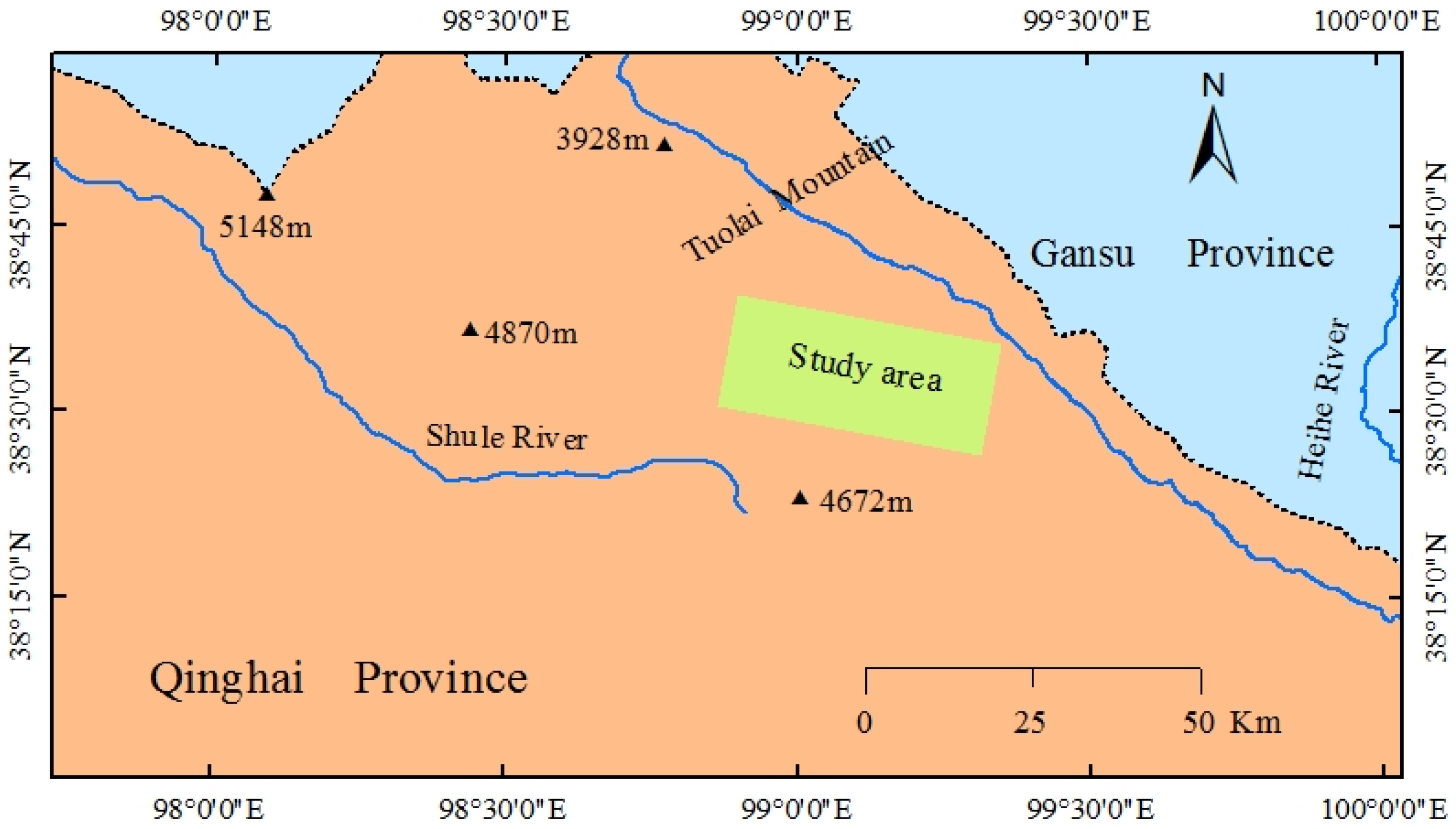
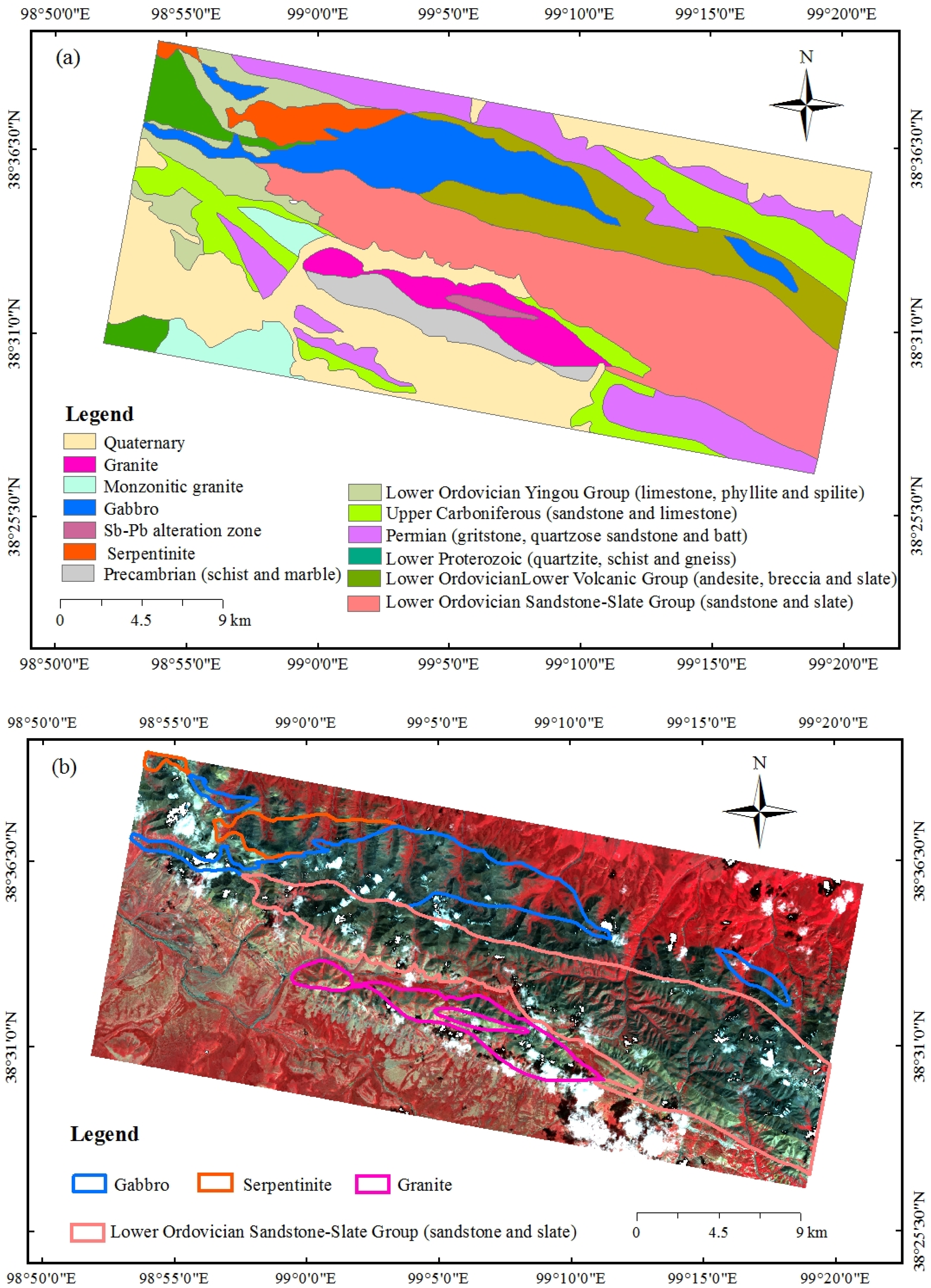
2.1. Study Area

The study area (Figure 1) is located within latitudes 38°10′ N and 38°45′ N and longitudes 98°45′ E and 99°30′ E, in the northern Qinghai Province of western China, which lies in the Chi-lien Mountains of the northern of Qinghai–Tibet Plateau. The region has a plateau continental climate and an approximate mean elevation of 4200 m, resulting in abundant snow and ice cover for most of the year. Vegetation in this area is mainly low grass. The summer season in the area occurs from June to August with minimal snow and ice cover. Despite the increasing vegetation cover associated with summer conditions, geological materials are best exposed during this time frame [11,49]. Therefore, this is the best period for remote sensing observations.

Based on fieldwork and remote sensing images, the study area was selected at locations where rocks were relatively well exposed, as shown in the compiled lithological map (Figure 2a), however, vegetation was still spotted, as visible in the false color composition (Figure 2b). The main rock types in this area include gabbro, serpentinite, granite, and quartzose rock, which are well exposed and are less covered by vegetation. In this area, gabbro, serpentinite, and granite are all intrusive rocks. Gabbro and serpentinite rocks are both the major components of mafic–ultramafic rocks, and are seldom distributed in lower volcanic groups of Ordovician age. Granitoids are the representative granite rocks, which are related to rare earth metals, the origin of nonferrous metals, and radioactive element ore deposits [11]. Sandstone is the major type of quartzose rock in this area and is mainly distributed in the lower Ordovician sandstone–slate group. Carbonate rocks are not widely exposed in the study area.

2.2. Dataset and Processing

One image of Landsat 8 OLI data (LC81340332014244LGN00) with few clouds provided by the USGS EROS data center (Sioux Falls, SD, USA) [46] was used in this study, and is detailed in

Table 1. Landsat 8 Operational Land Imager (OLI) band information.

Band Description	Wavelength ($\mathsf{\mu }m$)	Spatial Resolution (m)
Band 1 Coastal	0.433–0.453	30
Band 2 Blue	0.450–0.515
Band 3 Green	0.525–0.600
Band 4 Red	0.630–0.680
Band 5 NIR	0.845–0.885
Band 6 SWIR 1	1.560–1.660
Band 7 SWIR 2	2.100–2.300
Band 8 Pan	0.500–0.680	15

. The data were collected on 1 September 2014, close to the summer season (from June to August) to minimize snow and ice cover and maximize the exposure of rocks and minerals. The images acquired are Level 1 digital number data products, with radiation calibration and geometric correction methods previously applied. The data were processed as follows: (i) VNIR–SWIR images (band 1 to band 7, 30 m resolution) were radiometrically calibrated to obtain the top of atmosphere reflectance data; (ii) the Fast Line–of–Sight atmospheric analysis of spectral hypercubes (FLAASH) models were conducted for atmospheric correction to obtain surface reflectance data; (iii) the images were fused with the panchromatic band (band 8, 15 m resolution) to a spatial resolution of 15 m. The final reflectance images from VNIR to SWIR wavelengths, with a spatial resolution of 15 m, were used to derive texture images for lithological classification. All the procedures of data processing in this section were conducted in ENVI (ENVI5.2 SP 1, ITT Visual Information Solutions, Boulder, CO, USA, 2015).

Four rock types are discussed in this paper: gabbro, serpentinite, granite, and quartzose rocks, which are widely distributed within the earth’s crust and are well exposed in the study area. Rocks or minerals that are much covered by vegetation are not addressed in this paper, as the texture and spectral information would be concealed or impaired by vegetation. In addition, some samples of these rocks were selected based mainly on the geological map (Figure 2a). In addition, some remote sensing indices derived from the Advanced SpaceborneThermal Emission and Reflectance Radiometer (ASTER, National Aeronautics and Space Administration, Washington, DC, USA) imagery (i.e., $\left(\mathrm{b}12\times \mathrm{b}{14}^3\right)/\mathrm{b}{13}^4$, $\mathrm{b}13/\mathrm{b}12$) were also used as supplementary information for selecting samples of gabbro and quartzose rock. In fact, the method of choosing rock samples in this study is the same as that used in previous studies [11,49], and is detailed in Ding et al. [48].

3. Methods

3.1. Extraction and Analysis of Spatial Textural Features

3.1.1. Box-Counting Dimension Method to Extract Textural Features

The concept of fractal geometry, which was initially proposed by Mandelbrot [50], provides a simple method to describe the irregularities of complex objects and objects with self-similar characteristics at different scales (spatial, temporal, or otherwise) in nature. Remote sensing images are not only spectrally and spatially complex, but they often exhibit certain self-similarities at different scales [51]. Therefore, increasing attention has been paid to fractal geometry in the remote sensing community. Fractal models have been used in a variety of image processing and pattern recognition applications [52]. For example, they have been used to describe image texture and to segment various types of images [30,31,35,53]. In the past decades, fractal geometry has been one of the most popular techniques for texture extraction because of its robustness in image scaling [30,31,41,54]. Fractals characterize the roughness or geometric complexity of surface features in remote sensing images. Roughness or geometric complexity, which is related to surface morphology, plays an important role in improving image understanding and classification. Applications of fractal models to image analysis mainly depend on the estimation of the fractal dimension (𝐹𝐷) [52]. More generally, the more irregular an object is, the higher its 𝐹𝐷 value. Thus, $FD$ value is intimately linked to the concept of roughness or geometric complexity. In this way, different surface objects may have characteristic textures or roughness that could be measured by different $FD$ values. In this study, the box-counting method devised by Goodchild [54] was used to calculate the fractal dimension. This method divides an area into regular boxes with the same box edge length. Here, $M$ is the measured object, $\mathsf{\epsilon }$ is the box edge length, $M_{\mathsf{\epsilon }}\left(C\right)$ and $C$ is the lowest number of boxes in the grid divided curve and scales, respectively, and $FD$ is the fractal dimension of $M$.

$$FD=\underset{\mathsf{\epsilon }\to \infty }{\lim }\frac{\log M_{\mathsf{\epsilon }}\left(C\right)}{\log \mathsf{\epsilon }}$$

(1)

The value of $FD$ ranges from 1.0 to 2.0. To extract the fractal dimension of each pixel in remote sensing images, a 3 × 3 moving window covering the neighboring pixels is used. In this way, a new layer is generated as the texture image. Each pixel in this layer is assigned an $FD$ value.

3.1.2. Optimal Feature Combinations of Spectra and Textural Vectors

The texture images derived from seven spectral channels (VNIR–SWIR images) will yield hundreds of combinations of texture vectors for classification. Hence, feature selection has to be conducted before the image classification. Feature selection is a technique for selecting optimal combinations of vectors that consistently provide good performance in object classification [55]. In this paper, feature selection is conducted by three steps, including (i) selecting some criterion to evaluate the effectiveness of input vector in lithological classification; (ii) selecting vector combinations which have the best performance (or achieve to the defined standard); and (iii) setting the selected vectors as the optimal features, then feature selection is accomplished. Given that we were initially interested in whether the incorporation of textural features would aid spectral features to improve classification accuracy, different combinations of texture images, fused with all seven spectral bands, were examined to select the optimal input feature vectors.

The effectiveness of input feature vectors in lithological classification can be measured by the separability between two classes. The J–M distance has been mostly used for evaluating the separability between two classes [56,57,58] and was applied here to select the optimal feature vectors. The larger the class separability of the input vectors, the greater the J–M distance. The J–M distance is the average distance between two class-density functions, which is calculated using Equations (2) and (3).

$$J–M\left(i,j\right)=2\left(1-e^{-a}\right)$$

(2)

$$a=\frac{1}{8}{\left(m_i-m_j\right)}^T\left(\frac{2}{\left(C_j-C_i\right)}\right)\left(m_i-m_j\right)+\frac{1}{2}\ln \sqrt{\frac{\left|\left(C_j-C_i\right)/2\right|}{\left|C_i\right|·\left|C_j\right|}}$$

(3)

where $i\mathrm{and}j$ are the two classes being compared, $m_i$ and $m_j$ is the mean vector of class $i$ and $j$, respectively, and $C_i$ and $C_j$ is the covariance matrix of the feature response of class $i$ and $j$ respectively. The value of J–M ranges from 0.0 to 2.0, and measures the pairwise class separability. A large J–M distance value indicates higher class separability.

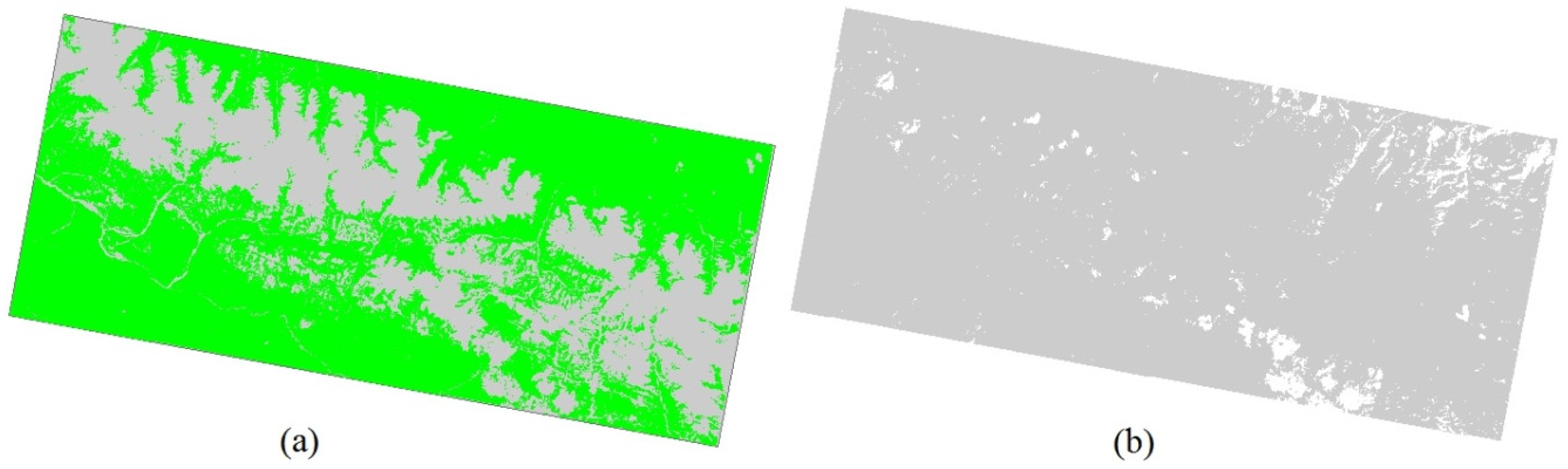
3.2. Interference Elimination in Remote Sensing Images

A few clouds were present in the used images, and need to be considered, as shown in Figure 2a. In this figure, vegetation is shown in red, while clouds, snow, and ice are presented in white. Textural features are described in terms of spatial variability associated with the digital numbers (DNs) of local pixels. Hence, vegetation and clouds in the image would conceal or impair the textural information. To eliminate interference from vegetation, the normalized difference vegetation index (NDVI) was calculated using Equation (4). Based on the statistical characterization of vegetation pixels from the NDVI image, the threshold value for NDVI was set as 0.4 to mark off the vegetation pixels, which are colored green in Figure 3a. Clouds have a relatively high reflectance in the NIR wavelength (band 5). Based on the statistical characterization of cloud pixels from the NIR reflectance image, the threshold of 0.35–1.0 was set to mark off the cloud pixels, as shown in white in Figure 3b. The pixels falsely labeled as cloud were mainly distributed on the bright valley walls (e.g., in the northeast corner of Figure 3b). The bright valley in this study area is mostly covered by vegetation. Since a mask of vegetation pixels was also used before image classification, the pixels falsely labeled as cloud will not influence the results.

$$NDVI=\frac{NIR-R}{NIR+R}=\frac{band5-band4}{band5+band4}$$

(4)

3.3. Support Vector Machine Classifier

SVM based on statistical learning theory (SLT) is one of the most popular learning algorithms for classification and has been intensively studied by Vapnik et al. [59,60,61,62]. Unlike traditional SLT, which is based on structural risk minimization (SRM), SVM is a new universal learning theory based on Empirical Risk Minimization (ERM). Given its excellent learning and generalization ability, SVM has been widely employed in many fields, such as financial forecasting, image processing, face detection, and handwritten digit recognition [63,64,65,66,67].

The basic method of SVM classification can be generalized by the following two steps [64]:

• Map all input vectors to a high-dimensional feature space based on the kernel function, which is either linear or nonlinear.
• Construct an optimal hyperplane based on support vectors to separate the data into two classes according to the theory of the least errors and maximal margin between the hyperplane and the closest training data. The training samples that are closest to the hyperplane are support vectors, whereas the others are uncorrelated for establishing the class divisions.

We define ($X_1$, $y_1$), ($X_2$, $y_2$), …, ($X_n$, $y_n$) as the input training samples, $X_iϵR^n$ as input vectors, and $y_iϵ\left(-1,1\right)$ as the decision value of the training sample for each class. In terms of support vectors, the decision rule defined by an optimal hyperplane classifying the input data is given by the following equation:

$$f\left(x\right)=sign\left({{\displaystyle \sum }}_{i=1}^n{y}_i{a}_{i}K\left(X,X_i\right)+b\right)$$

(5)

where $X=\left(x_1,x_2,\dots \dots x_n\right)$ represents the input, the vectors $X_i$ ($i=1,2,\dots \dots N$) are support vectors, $a_i$ and $b$ are specific parameters of the hyperplane, and $K\left(X,X_i\right)$ is the kernel function used to construct machines with different types of decision surfaces in the feature space.

The SVM has the ability to deal with multiple effective image features for optimal classification with a small training sample set [48,68], which is an appropriate method to integrate textural and spectral features for lithological classification in this study.

4. Results and Discussions

4.1. Spatial Textural Feature Analysis

4.1.1. Spatial Textural Feature Extraction

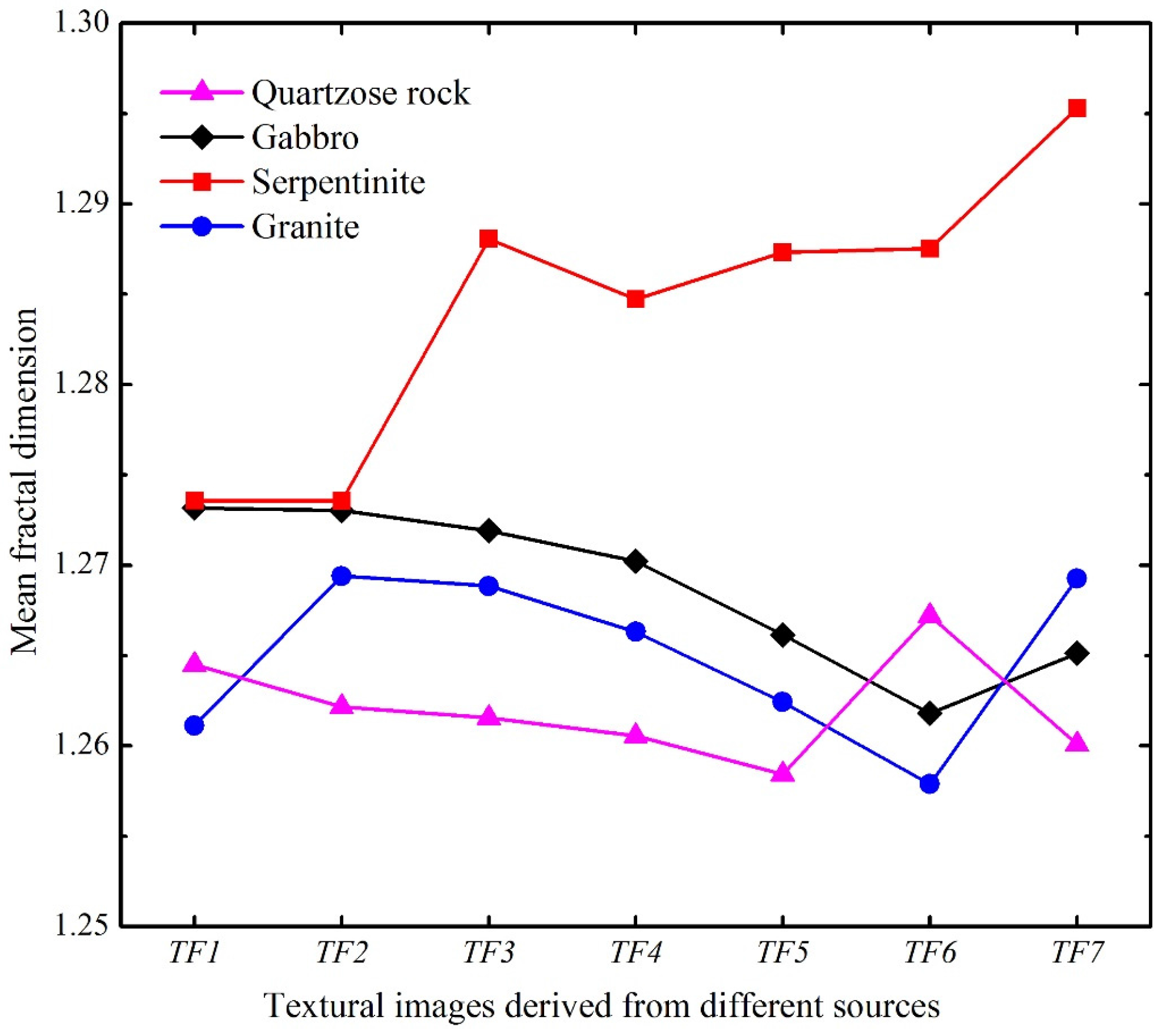
Seven texture images were derived from seven spectral bands of Landsat 8 data using the box-counting method. To examine the effectiveness of different texture images for lithological identification, the $FD$ values of the rock samples were extracted from the seven texture images, and the mean $FD$ value of each object is detailed in Figure 4.

Figure 4 provides the following information:

• On the whole, $FD$ shows a remarkable contrast between serpentinite and other rocks. The serpentinite has the highest $FD$, which means that its surface morphology is rougher than that of other rocks. In $TF1$ and TF2, the $FD$ values for gabbro and serpentinite are close, while from $TF3$ to $TF7$, there is an obvious difference between the $FD$ values for gabbro and serpentinite, which may result from the fact that texture images derived from different source data have a variable effect on rock identification.
• Regardless of the different texture images, different $FD$ values for the four rock types exist because of their different surface roughness, which would assist rock identification. From TF2 to TF6, the $FD$ values for gabbro and granite are almost the same, while for other pairwise rocks, the $FD$contrast is not immutable.

In conclusion, textural features measured by $FD$ may aid in separating certain different types of rocks. Texture images derived from different spectral bands have different sensitivities for lithological identification. Different texture images have varying abilities to identify the same pairs of rocks. For example, TF2 is not sufficient to distinguish gabbro from serpentinite, but it can be used to distinguish granite from quartzose rock in this example. Chen et al. [69] demonstrated that using only a single textural measured by fractal dimension is not effective to characterize objects in an image. Hence, it is necessary to examine the ability of different texture images and combinations of them before image classification.

4.1.2. Feature Vector Selection

In this study, our aim is to explore whether the incorporation of textural features can assist in distinguishing different silicate rocks. Hence, different combinations of texture images fused with all seven spectral features are examined. A total of 127 combinations of texture and spectral vectors are possible, as detailed in

Table 2. Different combinations of spectral and textural vectors ^a.

Rank	Series 1	Series 2	Series 3	Series 4	Series 5	Series 6	Series 7
1	SF + TF1	SF + TF12	SF + TF123	SF + TF1234	SF + TF12345	SF + TF123456	SF + TF1–7
2	SF + TF2	SF + TF13	SF + TF124	SF + TF1235	SF + TF12346	SF + TF123457	-
3	SF + TF3	SF + TF14	SF + TF125	SF + TF1236	SF + TF12347	SF + TF123467	-
4	SF + TF4	SF + TF15	SF + TF126	SF + TF1237	SF + TF12356	SF + TF123567	-
5	SF + TF5	SF + TF16	SF + TF127	SF + TF1245	SF + TF12357	SF + TF124567	-
6	SF + TF6	SF + TF17	SF + TF134	SF + TF1246	SF + TF12367	SF + TF134567	-
7	SF + TF7	SF + TF23	SF + TF135	SF + TF1247	SF + TF12456	SF + TF234567	-
8	-	SF + TF24	SF + TF136	SF + TF1256	SF + TF12457	-	-
9	-	SF + TF25	SF + TF137	SF + TF1257	SF + TF12467	-	-
10	-	SF + TF26	SF + TF145	SF + TF1267	SF + TF12567	-	-
11	-	SF + TF27	SF + TF146	SF + TF1345	SF + TF13456	-	-
12	-	SF + TF34	SF + TF147	SF + TF1346	SF + TF13457	-	-
13	-	SF + TF35	SF + TF156	SF + TF1347	SF + TF13467	-	-
14	-	SF + TF36	SF + TF157	SF + TF1356	SF + TF13567	-	-
15	-	SF + TF37	SF + TF167	SF + TF1357	SF + TF14567	-	-
16	-	SF + TF45	SF + TF234	SF + TF1367	SF + TF23456	-	-
17	-	SF + TF46	SF + TF235	SF + TF1456	SF + TF23457	-	-
18	-	SF + TF47	SF + TF236	SF + TF1457	SF + TF23467	-	-
19	-	SF + TF56	SF + TF237	SF + TF1467	SF + TF23567	-	-
20	-	SF + TF57	SF + TF245	SF + TF1567	SF + TF24567	-	-
21	-	SF + TF67	SF + TF246	SF + TF2345	SF + TF34567	-	-
22	-	-	SF + TF247	SF + TF2346	-	-	-
23	-	-	SF + TF256	SF + TF2347	-	-	-
24	-	-	SF + TF257	SF + TF2356	-	-	-
25	-	-	SF + TF267	SF + TF2357	-	-	-
26	-	-	SF + TF345	SF + TF2367	-	-	-
27	-	-	SF + TF346	SF + TF2456	-	-	-
28	-	-	SF + TF347	SF + TF2457	-	-	-
29	-	-	SF + TF356	SF + TF2467	-	-	-
30	-	-	SF + TF357	SF + TF2567	-	-	-
31	-	-	SF + TF367	SF + TF3456	-	-	-
32	-	-	SF + TF456	SF + TF3457	-	-	-
33	-	-	SF + TF457	SF + TF3467	-	-	-
34	-	-	SF + TF467	SF + TF3567	-	-	-
35	-	-	SF + TF567	SF + TF4567	-	-	-

^a The expression “SF + TF1–7” indicates the feature combination of seven spectral bands fused with TF1, TF2, TF3, TF4, TF5, TF6, and TF7. The same convention applies to the rest of the table contents.

. Then, the J–M distance is calculated between pairwise rocks to select the optimal combinations of input feature vectors, as shown in Figure 5. Figure 5 shows the feasibility of different vector combinations for lithological identification in the form of matrix. Each element (i, j) (here the i and j ranges from 1 to 7 and from 1 to 35, respectively) in the matrix indicates the vector combination in Series i and row j in Table 2. It needs to be noted that the element (0, 0) in the matrix (Figure 5) indicates the seven spectral vectors without textural features. The value of element (i, j) indicates the J–M distance between two classes. For example, element (3, 4) indicates the vector combination in Series 3 and row 4 in Table 2, namely SF + TF126; the value of element (3, 4) indicates the J–M distance between two classes calculated using the vector combination of SF + TF126. The matrices in Figure 5 were quantified using shades of color, which will help to visually distinguish the different performances of vector combinations in identifying pairwise rocks.

Figure 5 provides the following information:

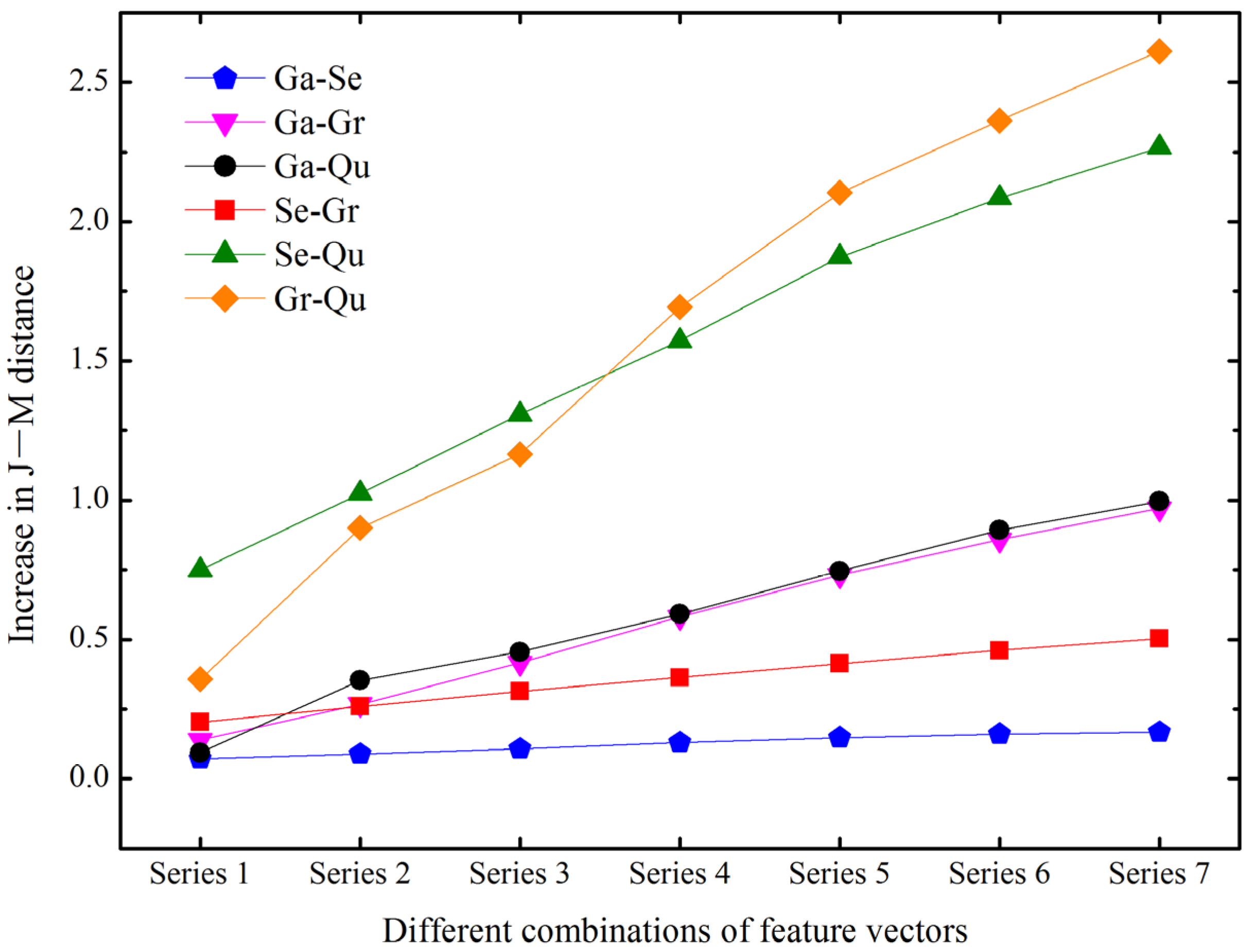
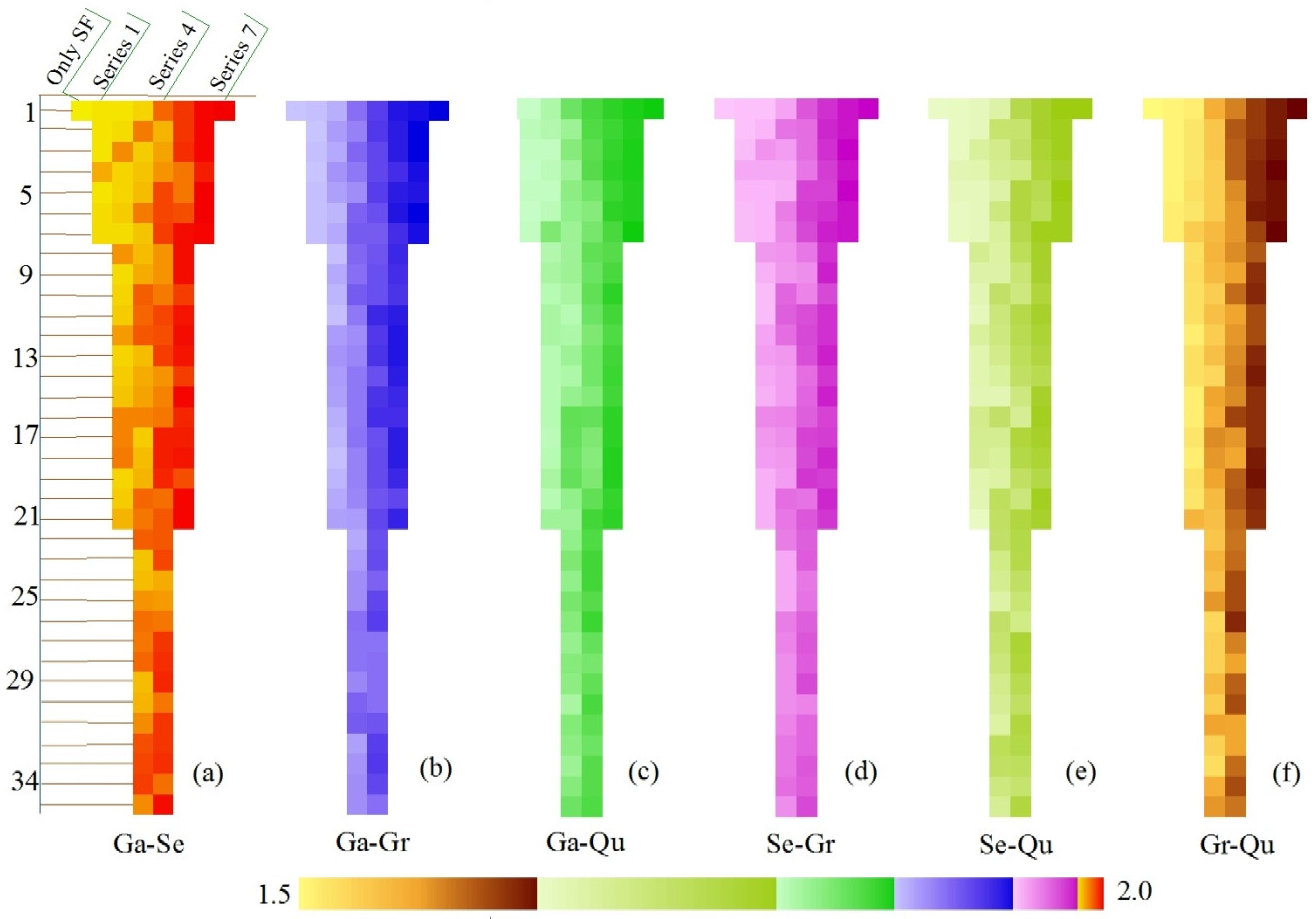
• For all six groups of pairwise rocks, the J–M distance increases significantly with the number of textural vectors, indicating that the incorporation of texture is useful for improving the identification of rocks. Moreover, for the same number of textural vectors, different combinations of them generate different J–M distances. The statistically significant J–M distances for the same number of vectors are detailed in

  Table 3. Statistically significant J–M distance for the same number of vectors ^a.

  Pairwise Rocks	Series 1	Series 2	Series 3	Series 4	Series 5	Series 6	Series 7
  Ga–Se	SF + TF4	SF + TF47	SF + TF467	SF + TF4567	SF + TF14567	SF + TF124567	SF + TF1–7
  Ga–Gr	SF + TF3	SF + TF15	SF + TF367	SF + TF1345	SF + TF13457	SF + TF123457	SF + TF1–7
  Ga–Qu	SF + TF2	SF + TF23	SF + TF234	SF + TF2367	SF + TF23567	SF + TF234567	SF + TF1–7
  Se–Gr	SF + TF4	SF + TF45	SF + TF146	SF + TF1467	SF + TF12467	SF + TF123467	SF + TF1–7
  Se–Qu	SF + TF4	SF + TF45	SF + TF456	SF + TF2456	SF + TF12456	SF + TF124567	SF + TF1–7
  Gr–Qu	SF + TF6	SF + TF67	SF + TF235	SF + TF2367	SF + TF23567	SF + TF123567	SF + TF1–7

  ^a Ga is gabbro, Se is serpentinite, Gr is granite, and Qu is quartzose rock; the expression SF + TF1234567 indicates the feature combination of seven spectral features fused with TF1, TF2, TF3, TF4, TF5, TF6, and TF7. The same convention applies to the rest of the table contents.

  . The textural vectors of $TF4,TF7,\mathrm{and}TF6$ had better performance in identifying gabbro–serpentinite, while $TF3,TF5,\mathrm{and}TF1$ were more effective in identifying gabbro–granite. The textural vectors of $TF2\mathrm{and}TF3$ were more effective for gabbro-quartzose rock; $TF4,TF6,\mathrm{and}TF1$ for serpentinite–granite; $TF4,TF5,\mathrm{and}TF6$ for serpentinite–quartzose rock; and $TF6,TF2,TF3,\mathrm{and}TF2$ were more effective for identifying granite–quartzose rock. For all six pairs of rocks, the J–M distance has the highest value when all seven vectors are incorporated.
• It is clear that gabbro–serpentinite has the largest J–M distance, followed by serpentinite–granite, gabbro–granite, gabbro–quartzose rock, serpentinite–quartzose rocks and granite–quartzose rocks, which suggests that textural features are more useful for identifying granite and quartzose rocks.

To further examine the performance of texture images in identifying different pairs of rocks, the increase in class separability for the seven series that have statistically significant J–M distances for the same numbers of feature vectors (Table 3) were calculated, as shown in Figure 6. The increase in class separability is, in fact, the difference in value of J–M distance between the seven series with the seven spectral vectors. It is evident that the incorporation of textural vectors has a remarkable effect on the following pairs of rocks: serpentinite–quartzose rock, granite–quartzose rock, gabbro–quartzose rock, and gabbro–granite. In particular, the textural vectors performed best on serpentinite–quartzose rock and granite–quartzose rock. For serpentinite–granite and gabbro–serpentinite, which can be well distinguished when only spectral vectors are used, the increase in class separability is insignificant.

The statistical results indicate that integrating spatial textural features with spectral features yields an improvement in rock separability, especially for granite and quartzose rock, which may result in improved classification accuracy. To confirm this premise, the vector combinations that achieved the most significant J–M distances were compared with the classification results obtained using only spectral vectors.

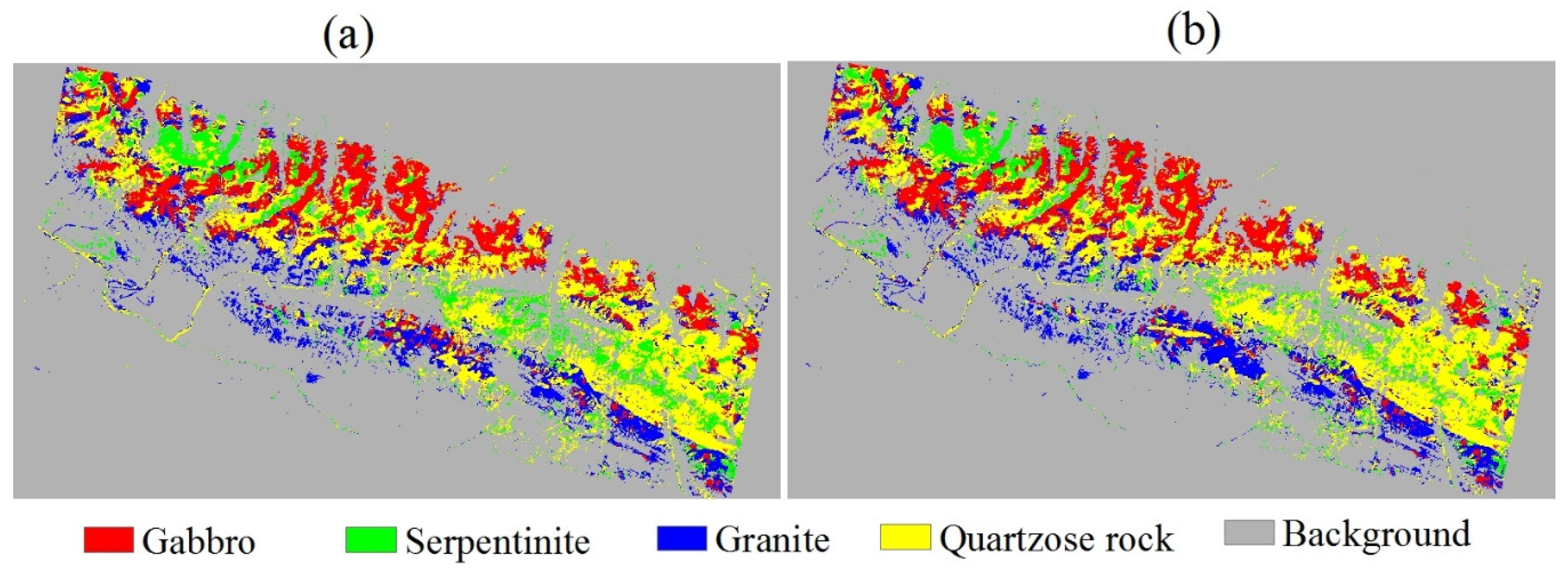
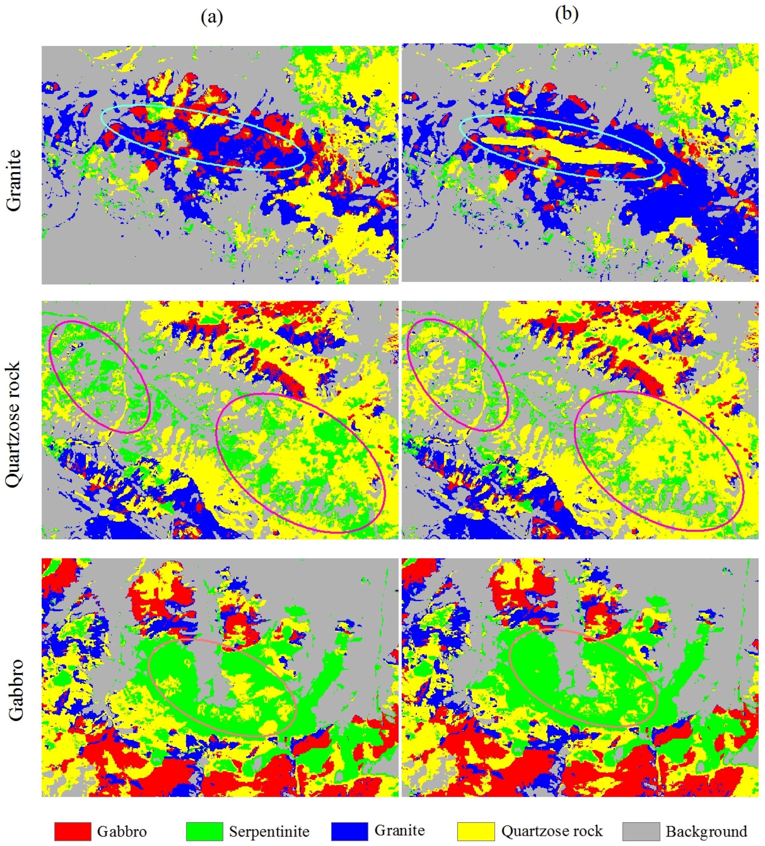
4.2. Lithological Classification Using Selected Features

The texture and spectral images acting as input vectors were fused in the SVM classifier for lithological classification. Then, the Landsat 8 imagery was classified into four rock types, including gabbro, serpentinite, granite, and quartzose rock. The classification results are shown in Figure 7 and Figure 8. The classification accuracy was calculated based on the confusion matrix and was presented in

Table 4. Confusion matrix and accuracy evaluation of classification results using support vector machine (SVM) with seven spectral vectors.

Class	Gabbro	Serpentinite		Granite		Quartzose Rock		Total
Gabbro	730	0		87		97		914
Serpentinite	0	250		0		93		343
Granite	26	85		120		553		784
Quartzose rock	13	0		120		39		172
Total	769	335		327		782		2213
Overall accuracy: 74.69%; κ: 0.6366
Class	Product Accuracy (%)		User Accuracy (%)		Commission (%)		Omission (%)
Gabbro	94.93 (730/769)		79.87 (730/914)		20.13 (184/914)		5.07 (39/769)
Serpentinite	74.63 (250/335)		72.89 (250/343)		27.11 (93/343)		25.37 (85/335)
Granite	36.70 (120/327)		69.77 (120/172)		30.23 (52/172)		63.30 (207/327)
Quartzose rock	70.72 (553/782)		70.54 (553/784)		29.46 (231/784)		29.28 (229/782)

and

Table 5. Confusion matrix and accuracy evaluation of classification results using SVM with seven spectral vectors fused with seven textural vectors.

Class	Gabbro	Serpentinite		Granite		Quartzose Rock		Total
Gabbro	731	0		120		45		896
Serpentinite	0	267		29		0		296
Granite	32	68		608		35		743
Quartzose rock	6	0		25		247		278
Total	769	335		782		327		2213
Overall accuracy: 83.73%; κ: 0.7682
Class	Product Accuracy (%)		User Accuracy (%)		Commission (%)		Omission (%)
Gabbro	95.06 (731/769)		81.58 (731/896)		18.42 (165/896)		4.94 (38/769)
Serpentinite	79.7 (267/335)		90.2 (267/296)		9.8 (29/296)		20.3 (68/335)
Granite	77.75 (608/782)		81.83 (608/743)		18.17 (135/743)		22.25 (174/782)
Quartzose rock	75.54 (247/327)		88.85 (247/278)		11.15 (31/278)		24.46 (80/327)

. The results show that the classification incorporating textural features is noticeably improved compared to that using only spectral vectors. The overall accuracy and Kappa coefficient ($\mathsf{\kappa }$) increased by 9.04% and 0.13%, respectively. Moreover, all four rock objects were better identified, especially granite and quartzose rocks, which had the highest increase in classification accuracy, confirming the results presented in Section 4.2.

Improved performance is achieved when the selected feature vectors are integrated in SVM for lithological classification. This can be attributed to two factors. First, texture features improve our understanding of images, as they characterize the roughness or geometric complexity of objects in the remote sensing image. Second, the optimal combination of feature vectors is selected to act as the input vectors in a classifier. However, the universality of this strategy needs to be confirmed further. Only four common rock types are discussed in this paper, due to the limited size of the study area. Larger areas with additional rock types should also be taken into consideration. The concept of texture has been successfully introduced in remote sensing science. Textural features help to better characterize the surface morphology of surface objects. In future studies, other surface parameters related to the physical or chemical properties of rocks should be considered for lithological identification, such as permittivity, thermal characteristics, albedo, and indices related to rock chemical components. In addition, the geographical environment, especially land surface temperature and atmospheric moisture content, may influence the surface morphology of rocks [48], such as changed surface structural characteristics, which may result from sedimentation occurring within weathered fractures. The geographic environment in a specific study area may limit the robustness of this strategy, which would also limit the accuracy of image classification. Hence, for other regions or other rock types, more analysis and validation is necessary.

5. Conclusions

Prior studies have demonstrated the capability of integrating textural features with spectral features for image classification and pattern recognition. However, these studies focus mostly on the improvement or design of texture-derived methods. In addition, the used textural features are calculated from a single remote sensing image, resulting in invalid results, which has been demonstrated in Chen et al. [69] . In this paper, we focused on examining the sensitivity of different texture images to aid spectral features for lithological classification. So, the J–M distance was used to examine the performance of textural vectors derived from different sources and to select optimal combinations of textural and spectral vectors for lithology identification. The statistical results indicate that more textural vectors yield higher class separability. Then, multiple textural vectors and multiple spectral vectors were integrated using the SVM model to improve lithological classification. Classification results were evaluated based on the confusion matrix. Compared with conventional classification based only on spectral features, the classification accuracy obtained by integrated textural and spectral features is noticeably improved, especially for granite and quartzose rocks, which show an increase in classification accuracy of 38.84% and 7.03%, respectively, indicating that textural features provide useful supplementary information for lithological identification. We conclude that (i) textural features that reveal rock differences in surface morphology have a remarkable ability to improve lithological classification, especially for rocks that have subtle spectral features; (ii) texture images derived from different data sources have different sensitivities for lithological identification. So, the use of multiple textural vectors has a better performance than that of a single textural vector to aid spectral information for lithological classification; (iii) it is necessary to select optimal feature vector combinations using appropriate methods, such as the J–M distance. Furthermore, more useful indicators, similar to the textural features derived from remote sensing imagery, need to be explored and integrated with spectral features using suitable classifiers to improve the accuracy of lithological classification. Nevertheless, we propose a referable technique to improve the classification of silicate rocks by fusing textural features with spectral features, which will aid in lithological mapping at macroscopic scales and guide further geological exploration in harsh natural environments.

References

1. BenDor, E.; Inbar, Y.; Chen, Y. The reflectance spectra of organic matter in the visible near-infrared and short wave infrared region (400–2500 nm) during a controlled decomposition process. Remote Sens. Environ. 1997, 61, 1–15. [Google Scholar] [CrossRef]
2. Grove, C.I.; Hook, S.J.; Paylor, E.D. Laboratory Reflectance Spectrum of 160 Minerals, 0.4–2.5 Micron; JPL Publication 92-2; Jet Propulsion Laboratory: La Cañada Flintridge, CA, USA, 2010. [Google Scholar]
3. Abrams, M.; Goetz, A.; Kahle, A.; Ashley, R.; Rowan, L. Mapping of hydrothermal alteration in the Cuprite mining district, Nevada, using aircraft scanner images for the spectral region 0.46 to 2.36 μm. Geology 1978, 5, 713–718. [Google Scholar] [CrossRef]
4. Thompson, A.J.B.; Hauff, P.L.; Robitaille, A.J. Alteration mapping in exploration: Application of short-wave infrared SWIR spectroscopy. Soc. Econ. Geol. 1999, 39, 16–27. [Google Scholar]
5. Ninomiya, Y.; Fu, B. Quartz Index, Carbonate index and SiO2 content index defined for ASTER TIR data. J. Remote Sens. Soc. Jpn. 2002, 22, 50–61. [Google Scholar]
6. Rockwell, B.W.; Hofstra, A.H. Identification of quartz and carbonate minerals across northern Nevada using ASTER thermal infrared emissivity data—Implications for geologic mapping and mineral resource investigations in well-studied and frontier areas. Geosphere 2008, 4, 992–992. [Google Scholar] [CrossRef]
7. Oztan, N.S.; Suzen, M.L. Mapping evaporate minerals by ASTER. Int. J. Remote Sens. 2011, 32, 1651–1673. [Google Scholar] [CrossRef]
8. Bertoldi, L.; Massironi, M.; Visona, D.; Carosi, R.; Montomoli, C.; Gubert, F.; Naletto, G.; Pelizzo, M.G. Mapping the Buraburi granite in the Himalaya of Western Nepal: Remote sensing analysis in a collisional belt with vegetation cover and extreme variation of topography. Remote Sens. Environ. 2011, 115, 1129–1144. [Google Scholar] [CrossRef]
9. Honarmand, M.; Ranjbar, H.; Shahabpour, J. Application of principal component analysis and spectral angle mapper in the mapping of hydrothermal alteration in the Jebal-Barez area, southeastern Iran. Resour. Geol. 2012, 62, 119–139. [Google Scholar] [CrossRef]
10. Pournamdari, M.; Hashim, M. Detection of chromite bearing mineralized zones in Abdasht ophiolite complex using ASTER and ETM+ remote sensing data. Arab. J. Geosci. 2014, 7, 1973–1983. [Google Scholar] [CrossRef]
11. Ding, C.; Li, X.Q.; Liu, X.N.; Zhao, L.T. Quartzose-mafic spectral feature space model: A methodology for extracting felsic rocks with ASTER thermal infrared radiance data. Ore Geol. Rev. 2015, 66, 283–292. [Google Scholar] [CrossRef]
12. Peres, L.F.; Dacamara, C.C. Land surface temperature and emissivity estimation based on the two-temperature method: Sensitivity analysis using simulated MSG/SEVIRI data. Remote Sens. Environ. 2004, 91, 377–389. [Google Scholar] [CrossRef]
13. Chen, X.; Warner, T.A.; Campagna, D.J. Integrating visible, near-infrared and short-wave infrared hyperspectral and multispectral thermal imagery for geological mapping at Cuprite, Nevada. Remote Sens. Environ. 2007, 110, 344–356. [Google Scholar] [CrossRef]
14. Li, Z.L.; Tang, B.H.; Wu, H.; Ren, H.; Yan, G.; Wan, Z.; Trigo, I.F.; Sobrino, J.A. Satellite-derived land surface temperature: Current status and perspectives. Remote Sens. Environ. 2013, 131, 14–37. [Google Scholar] [CrossRef]
15. Collins, A.H. Thermal infrared-spectra and images of altered volcanic-rocks in the virginia range, Nevada. Int. J. Remote Sens. 1991, 12, 1559–1574. [Google Scholar] [CrossRef]
16. Hook, S.J.; Gabell, A.R.; Green, A.A.; Kealy, P.S. A comparison of techniques for extracting emissivity information from thermal infrared data for geologic studies. Remote Sens. Environ. 1992, 42, 123–135. [Google Scholar] [CrossRef]
17. Satterwhite, M.B.; Henley, J.P.; Carney, J.M. Effects of lichens on the reflectance spectra of granitic rock surfaces. Remote Sens. Environ. 1985, 18, 105–112. [Google Scholar] [CrossRef]
18. An, P.; Chung, C.F.; Rencz, A.N. Digital lithology mapping from airborne geophysical and remote sensing data in the Melville Peninsula, Northern Canada, using a neural network approach. Remote Sens. Environ. 1995, 53, 76–84. [Google Scholar] [CrossRef]
19. Ryherd, S.; Woodcock, C. Combining spectral and texture data in the segmentation of remotely sensed images. Photogramm. Eng. Remote Sens. 1996, 62, 181–194. [Google Scholar]
20. Sabins, F.F. Remote sensing for mineral exploration. Ore Geol. Rev. 1999, 14, 157–183. [Google Scholar] [CrossRef]
21. Grebby, S.; Cunningham, D.; Naden, J.; Tansey, K. Lithological mapping of the Troodos ophiolite, Cyprus, using airborne LiDAR topographic data. Remote Sens. Environ. 2010, 114, 713–724. [Google Scholar] [CrossRef] [Green Version]
22. Van der Meer, F.D.; Van der Werff, H.M.A.; Van Ruitenbeek, F.J.A.; Hecker, C.A.; Bakker, W.H.; Noomen, M.F.; Van der Meijde, M.; Carranza, E.J.M.; Smeth, J.B.D.; Woldai, T. Multi- and hyperspectral geologic remote sensing: A review. Int. J. Appl. Earth Obs. 2012, 14, 112–128. [Google Scholar] [CrossRef]
23. Othman, A.; Gloaguen, R. Comparison of Different Machine Learning Algorithms for Lithological Mapping Using Remote Sensing Data and Morphological Features: A Case Study in Kurdistan Region, NE Iraq; EGU: Munich, Germany, 2015. [Google Scholar]
24. Haralick, R.M.; Shanmugam, K.; Dinstein, I.H. Textural features for image classification. IEEE Trans. Syst. Man Cybern. 1973, 3, 610–621. [Google Scholar] [CrossRef]
25. Barber, D.G.; Ledrew, E.F. SAR sea ice discrimination using texture statistics—A multivariate approach. Photogramm. Eng. Remote. Sens. 1991, 57, 385–395. [Google Scholar]
26. Coburn, C.A.; Roberts, A.C.B. A multiscale texture analysis procedure for improved forest stand classification. Int. J. Remote Sens. 2004, 25, 4287–4308. [Google Scholar] [CrossRef]
27. Su, H.; Wang, Y.; Xiao, J.; Yan, X.-H. Classification of MODIS images combining surface temperature and texture features using the Support Vector Machine method for estimation of the extent of sea ice in the frozen Bohai Bay, China. Int. J. Remote Sens. 2015, 36, 2734–2750. [Google Scholar]
28. Fan, H. Land-cover mapping in the Nujiang Grand Canyon: Integrating spectral, textural, and topographic data in a random forest classifier. Int. J. Remote Sens. 2013, 34, 7545–7567. [Google Scholar] [CrossRef]
29. Kittler, J. Processing for Remote Sensing. Philos. Trans. R. Soc. Lond. 1983, 309, 323–335. [Google Scholar] [CrossRef]
30. Wood, E.M.; Pidgeon, A.M.; Radeloff, V.C.; Keuler, N.S. Image texture as a remotely sensed measure of vegetation structure. Remote Sens. Environ. 2012, 121, 516–526. [Google Scholar] [CrossRef]
31. Mather, P.M.; Tso, B.; Koch, M. An evaluation of Landsat TM spectral data and SAR-derived textural information for lithological discrimination in the Red Sea Hills, Sudan. Int. J. Remote Sens. 1998, 19, 587–604. [Google Scholar] [CrossRef]
32. Chica-Olmo, M.; Abarca-Hernández, F. Computing geostatistical image texture for remotely sensed data classification. Comput. Geosci. 2000, 26, 373–383. [Google Scholar] [CrossRef]
33. Franklin, S.E.; Maudie, A.J.; Lavigne, M.B. Using spatial co-occurrence texture to increase forest structure and species composition classification accuracy. Photogramm. Eng. Remote Sens. 2001, 67, 849–855. [Google Scholar]
34. Li, P.; Li, Z.; Moon, W.M. Lithological discrimination of Altun area in northwest China using Landsat TM data and geostatistical textural information. Geosci. J. 2001, 5, 293–300. [Google Scholar] [CrossRef]
35. Corresponding, P.D.; Leblon, B. Rock unit discrimination on Landsat TM, SIR-C and Radarsat images using spectral and textural information. Int. J. Remote Sens. 2004, 25, 3745–3768. [Google Scholar]
36. Jakob, S.; Bühler, B.; Gloaguen, R.; Breitkreuz, C.; Ali Eliwa, H.; El Gameel, K. Remote sensing based improvements of the geological maps of the Neoproterozoic Ras Gharib segment in the Easter Desert (NE-Egypt) using texture features. J. Afr. Earth Sci. 2015, 111, 138–147. [Google Scholar] [CrossRef]
37. Qari, M. Application of landsat TM data to geological studies, al-khabt area, southern arabian shield. Photogramm. Eng. Remote Sens. 1991, 57, 421–429. [Google Scholar]
38. Nalbant, S.S.; Alptekin, O. The use of Landsat Thematic Mapper imagery for analyzing lithology and structure of korucu-dugla area in western turkey. Int. J. Remote Sens. 1995, 16, 2357–2374. [Google Scholar] [CrossRef]
39. Rajesh, H.M. Mapping Proterozoic unconformity-related uranium deposits in the Rockhole area, Northern Territory, Australia using landsat ETM. Ore Geol. Rev. 2008, 33, 382–396. [Google Scholar] [CrossRef]
40. Pan, W.; Ni, G.; Li, H. A study of RS image landform frame and lithologic component decomposing algorithm and multifractal feature of rock types. Earth Sci. Front. 2009, 16, 248–256. [Google Scholar] [CrossRef]
41. Wang, X.; Niu, R.; Wu, T. Research on lithology intelligent classification for Three Gorges Reservoir area. Rock Soil Mech. 2010, 31, 2946–2950. [Google Scholar]
42. Xiong, Y.; Khan, S.D.; Mahmood, K.; Sisson, V.B. Lithological mapping of Bela ophiolite with remote-sensing data. Int. J. Remote Sens. 2011, 32, 4641–4658. [Google Scholar] [CrossRef]
43. Zoheir, B.; Emam, A. Integrating geologic and satellite imagery data for high-resolution mapping and gold exploration targets in the South Eastern Desert, Egypt. J. Afr. Earth Sci. 2012, 66–67, 22–34. [Google Scholar] [CrossRef]
44. He, J.; Harris, J.R.; Sawada, M.; Behnia, P. A comparison of classification algorithms using Landsat-7 and Landsat-8 data for mapping lithology in Canada’s Arctic. Int. J. Remote Sens. 2015, 36, 2252–2276. [Google Scholar] [CrossRef]
45. Roy, D.P.; Wulder, M.A.; Loveland, T.R.; Woodcock, C.E.; Allen, R.G.; Anderson, M.C.; Helder, D.; Irons, J.R.; Johnson, D.M.; Kennedy, R.; et al. Landsat-8: Science and product vision for terrestrial global change research. Remote Sens. Environ. 2014, 145, 154–172. [Google Scholar] [CrossRef]
46. United States Geological Survey (USGS) and Earth Resources Observation and Science (EROS) data center. Available online: http://glovis.usgs.gov/ (accessed on 6 May 2016).
47. Marceau, D.J.; Howarth, P.J.; Dubois, J.M.M.; Gratton, D.J. Evaluation of The Grey-level Co-Occurrence Matrix Method for Land-Cover Classification Using Spot Imagery. IEEE Trans. Geosci. Remote Sens. 1990, 28, 513–519. [Google Scholar] [CrossRef]
48. Cai, S.; Zhang, R.; Liu, L.; Zhou, D. A method of salt-affected soil information extraction based on a support vector machine with texture features. Math. Comput. Model. 2010, 51, 1319–1325. [Google Scholar] [CrossRef]
49. Ding, C.; Liu, X.; Liu, W.; Liu, M.; Li, Y. Mafic-ultramafic and quartz-rich rock indices deduced from ASTER thermal infrared data using a linear approximation to the Planck function. Ore Geol. Rev. 2014, 60, 161–173. [Google Scholar] [CrossRef]
50. Mandelbrot, B.B. Fractals: Form, Chance and Dimension; W.H. Freeman and Company: San Francisco, CA, USA, 1977. [Google Scholar]
51. Lam, N.S.-N.; Cola, L.D. Fractals in Geography; Prentice Hall: Englewood Cliffs, NJ, USA, 1993. [Google Scholar]
52. Sun, W.; Xu, G.; Liang, P.G.S. Fractal analysis of remotely sensed images: A review of methods and applications. Int. J. Remote Sens. 2006, 27, 4963–4990. [Google Scholar] [CrossRef]
53. Myint, S.W. Fractal approaches in texture analysis and classification of remotely sensed data: Comparisons with spatial autocorrelation techniques and simple descriptive statistics. Int. J. Remote Sens. 2003, 24, 1925–1947. [Google Scholar] [CrossRef]
54. Goodchild, M.F. Fractals and the accuracy of geographical measures. Math. Geol. 1980, 12, 85–98. [Google Scholar] [CrossRef]
55. Proctor, C.; He, Y.; Robinson, V. Texture augmented detection of macrophyte species using decision trees. ISPRS J. Photogramm. 2013, 80, 10–20. [Google Scholar] [CrossRef]
56. Richards, J.A. Remote Sensing Digital Image Analysis: An Introduction; Springer: Heidelberg, Germany, 1986; pp. 47–54. [Google Scholar]
57. Adam, E.; Mutanga, O. Spectral discrimination of papyrus vegetation (Cyperus papyrus L.) in swamp wetlands using field spectrometry. ISPRS J. Photogramm. 2009, 64, 612–620. [Google Scholar] [CrossRef]
58. Ma, N.; Hu, Y.; Zhuang, D.; Wang, X. Determination on the optimum band combination of HJ-1A hyperspectral data in the case region of dongguan based on optimum index factor and J–M distance. Remote Sens. Technol. Appl. 2010, 25, 358–365. [Google Scholar]
59. Boser, B.E.; Guyon, I.M.; Vapnik, V.N. A training algorithm for optimal margin classifiers. In Proceedings of the Fifth Annual Workshop on Computational Learning Theory, Pittsburgh, PA, USA, 27–29 July 1992.
60. Cortes, C.; Vapnik, V. Support-vector networks. Mach. Learn. 1995, 20, 273–297. [Google Scholar] [CrossRef]
61. Schölkopf, B.; Burges, C.; Vapnik, V. Extracting support data for a given task. In Proceedings of the First International Conference on Knowledge Discovery and Data Mining, Montreal, PQ, Canada, 20–21 August 1995; AAAI Press: palo alto, CA, USA; pp. 252–257.
62. Vapnik, V.N. The Vicinal Risk Minimization Principle and the SVMs. In The Nature of Statistical Learning Theory, 2nd ed.; Springer: Heidelberg, Germany, 1999. [Google Scholar]
63. Mukherjee, S.; Osuna, E.; Girosi, F. Nonlinear prediction of chaotic time series using support vector machines. In Proceedings of the IEEE Workshop on Neural Networks for Signal Processing VII, Amelia Island, FL, USA, 24–26 September 1997; pp. 511–520.
64. Osuna, E.; Freund, R.; Girosi, F.; Ieee Comp, S.O.C. Training support vector machines: An application to face detection. In Proceedings of the IEEE Computer Society Conference on Computer Vision and Pattern Recognition, San Juan, Puerto Rico, USA, 17–19 June 1997; pp. 130–136.
65. Cai, Y.D.; Zhou, G.P.; Chou, K.C. Support vector machines for predicting membrane protein types by using functional domain composition. Biophys. J. 2003, 84, 3257–3263. [Google Scholar] [CrossRef]
66. Akay, M.F. Support vector machines combined with feature selection for breast cancer diagnosis. Expert Syst. Appl. 2009, 36, 3240–3247. [Google Scholar] [CrossRef]
67. Azar, A.T.; El-Said, S.A. Performance analysis of support vector machines classifiers in breast cancer mammography recognition. Neural Comput. Appl. 2014, 24, 1163–1177. [Google Scholar] [CrossRef]
68. Waske, B.; Van, D.L.S. Classifying multilevel imagery from SAR and optical sensors by decision fusion. IEEE Trans. Geosci. Remote Sens. 2008, 46, 1457–1466. [Google Scholar] [CrossRef]
69. Chen, Y.Q.; Bi, G. On texture classification using fractal dimension. Int. J. Pattern Recognit. Artif. Intell. 1999, 13, 929–943. [Google Scholar] [CrossRef]
Figure 1. Location of study area.
Applsci 06 00283 g001
Figure 2. (a) Generalized lithological map of the study area, showing the major lithology boundaries, modified after Ding et al. [49], Copyright 2014, Elsevier; and (b) false color composition with R = band 5 (near-infrared (NIR), 0.845–0.885), G = band 4 (Red, 0.630–0.680), and B = band 3 (Green, 0.525–0.600) in the study area with the lithological boundaries of gabbro, serpentinite, granite and Lower Ordovician Sandstone–Slate Group derived from Figure 2 (a) to highlight the distribution of the discussed rock types in this paper.
Applsci 06 00283 g002
Figure 3. (a) Vegetation pixels in green with 0.4 < normalized difference vegetation index (NDVI) < 1.0; and (b) cloud pixels in white with 0.35 < reflectance of NIR < 1.0 in the study area.
Applsci 06 00283 g003
Figure 4. Mean fractal dimension ( F D ) value for the four rock types in seven texture images ( T F i represents textural feature image derived from spectral band i ).
Applsci 06 00283 g004
Figure 5. J–M distance of pairwise rocks in different combinations of texture and spectral vectors. Ga is gabbro, Se is serpentinite, Gr is granite, and Qu is quartzose rock. The labels in (a) also apply to (bf). Different colors in this figure means the different J–M distance. A darker shades of color means a larger J–M distance.
Applsci 06 00283 g005
Figure 6. Increases in class separability for seven series compared to results obtained using only spectral vectors. Ga is gabbro, Se is serpentinite, Gr is granite, and Qu is quartzose rock.
Applsci 06 00283 g006
Figure 7. Landsat 8 classification results of the study area using (a) support vector machine (SVM) with only seven spectral vectors and no textural vector (the overall accuracy is 74.69% and κ is 0.64); and (b) SVM with seven textural vectors fused with seven spectral vectors (overall accuracy is 83.73% and κ is 0.77).
Applsci 06 00283 g007
Figure 8. Zoom-in and comparison of classification results of (a) SVM with seven spectral vectors and no textural feature; and (b) SVM with seven spectral vectors fused with seven textural vectors for gabbro, quartzose rock, and granite. The ellipses are used to highlight the changes between Figure 8 (a) and (b).
Applsci 06 00283 g008