Analysis and Evaluation of Performance Gains and Tradeoffs for Massive MIMO Systems

Abstract

Massive MIMO technique offers significant performance gains for the future of wireless communications via improving the spectral efficiency, energy efficiency and the channel quality with simple linear processing such as maximum-ratio transmission (MRT) or zero-forcing (ZF) by providing each user a large degree of freedom. In this paper, the system performance gains are studied in a multi-cell downlink massive MIMO system under the main considerations such as perfect channel estimation, imperfect channel estimation and the effect of interference among cells due to pilot sequences contamination. Then, mathematical expressions are derived for these gains i.e., spatial multiplexing gain, array gain and spatial diversity gain. After that, essential tradeoffs among these gains are considered under the effect of non-orthogonal interference, these tradeoffs are: spatial diversity gain vs. spatial multiplexing gain and array gain vs. spatial multiplexing gain. Simulation results show that the unbounded number of base station antennas boosts the array gain through concentrating the energy to spatial directions where users are sited, hence diminishing loss in array gain due to pilot contamination. The simulation results reveal also that massive MIMO strengthens the spatial multiplexing gain through increasing the number of served users via the same system resources in spite the effect of inter-cell interference. Finally, the spatial diversity gain is measured in term of outage probability and the simulation results show that raising the number of antennas will improve the outage probability. Meanwhile increasing the number of served users will lead to degrade the outage probability per user due to non-orthogonal interference from other cells.

1. Introduction

Communication in wireless channels is affected by multipath fading which causes a random fluctuation in the received signal power. This random fluctuation in signal level is known as fading, which affects the quality and reliability of wireless communication. Therefore, the need for a high data rate and high reliability is extremely challenging. One of the key technologies to increase network throughput by spatially exploiting more spectrum is achieved with MIMO technology. The leverages of MIMO are achieved through utilizing the spatial dimensions (submitted by the multiple antennas at the transmitter and the receiver) [1], where it was first investigated in point to point MIMO or single user MIMO which is called (SU-MIMO). However, the conventional MIMO system needs more effort to exploit the spatial multiplexing gains due to signal levels are exposed to the attenuation at cell edges as compared to interference levels there. A substitute for a point-to-point MIMO system is a multiuser MIMO system (MU-MIMO) in which an antenna array simultaneously serves multiple terminals independently. Then, the multiplexing throughput gains are shared among these terminals under line-of-sight propagation conditions, multiplexing gains can disappear for point-to-point MIMO but are retained in the multi-user system provided the angular separation of the users beyond the Rayleigh resolution of the array [2].

When the base station is equipped with a hundred antennas or more, better and more reliable communication is achieved. With very large MIMO system “Massive MIMO”, offers excess degrees of freedom that can be used to make sure that noise, fading and hardware imperfections vanished when signals from a large number of antennas are collected in the air jointly. The same property that makes massive MIMO flexible against fading also makes the technology very resistant to failure of one or a few of the antenna units. Massive MIMO can increase the capacity 10 times or more, can improve the radiated energy efficiency in order of 100 times, and can improve the quality of the received signal and achieve the link reliability [3,4].

The complexity scale in a conventional MIMO system concentrates at the uplink side because the main challenge of the conventional MIMO receiver is how to eliminate the multi-stream interference (MSI) since there are multiple streams from the individual transmit antennas interfere with each other at the receiver side. The multi-stream signal can be detected in a conventional MIMO system using linear equalization schemes such as Zero-Forcing (ZF) and Minimum Mean Squared Error (MMSE) which they are preferred for their less complexity scale; however, these schemes tend to suffer from poor bit error rate (BER) performance. While the nonlinear and the optimal receiver scheme is the Maximum likelihood (ML) detector, which exhibits higher performance, but the high computational complexity of this detector has made it inconsistent for widespread adoption in practical MIMO receiver designs when higher order constellations and a large number of antennas are used [5,6]. On the other hand, the complexity scale in massive MIMO system depends on which duplex system is used for the communication channel. When massive MIMO uses TDD principle, both uplink and downlink are used the same frequency spectrum but different time slots. At the uplink side, K-users send K-orthogonal pilot sequences to the base station for estimating the channels, while at the downlink side, using the concept of channel reciprocity base station utilizes the estimated channel at the uplink side to precode the transmit symbols. Hence, the complexity scale for the training process needs a minimum of 2K channel uses. However, when the massive system uses FDD principle, K-users transmit K-orthogonal pilot sequences to the base station for estimating the channels. At downlink side, the M-base station antennas transmit M-orthogonal pilot sequences to K-users; each user will estimate the channel then feeds back its channel estimates to the base station. Therefore, the complexity scale for the channel estimation process needs at least M + K channel uses in the uplink and M channel uses in the downlink [7].

Three main performance gains can be achieved under massive MIMO system: array gain, spatial diversity gain and spatial multiplexing gain. An increase in the energy efficiency means that the received SNR is increased from the coherent combining of the signals toward where users are located. Massive MIMO can improve the coverage area and resistance to noise through the use of array gain. An improvement in the quality and reliability of a wireless link means that the use of multiple antennas at base station is providing a receiver with multiple copies of the transmitted signal, and as a result the probability of one of the copies is not experiencing a deep fade increases, so the massive MIMO can provide a robust wireless link through spatial diversity gain. A linear increasing in data rate means that with large number of antennas many tens of terminals can be served simultaneously within the same bandwidth using the same transmit power, so the overall spectral efficiency can be ten times higher than in conventional MIMO [8], i.e., the massive MIMO can achieve high spectral efficiency through spatial multiplexing gain. Massive MIMO can achieve these performance gains individually by proper signal processing and channel coding. All these gains depend on statistical properties of massive MIMO channel and tradeoffs among these performance gains will appear significantly.

In massive MIMO system, the propagation losses due to coherent beamforming/combining are mitigated by the large number of antennas at the base station (i.e., a large array gain) [9]. With a large array gain, the transmitted power is reduced which leads to save terminals batteries on the uplink and reduces the power consumption by BS [10]. High spectral efficiencies are achieved per cell by scheduling many terminals for simultaneous transmission through exploiting the spatial multiplexing gain while the spectral efficiency per terminal might only be 1–4 bit/s/Hz [11]. Massive MIMO depends on reciprocity concept of time duplex division (TDD) system to create the precoding matrix for downlink transmission where the reverse channel is used to obtain the channel state information (CSI) of the forward channel, i.e., terminals send orthogonal pilot sequences in the uplink training. In multi-cell massive MIMO system, the same pilot sequences are re-used where the base station in one cell is polluted by users in other cells. This non-orthogonal nature is named pilot contamination [12], which causes CSI delay and channel estimation error between reverse channel estimation and forward channel data transmission which degrades the system performance gains significantly. CSI delay and channel estimation error cause diversity gain loss and array gain loss respectively [13,14].

The authors of [8] derived expressions to quantify the amount of antenna gain, diversity gain and multiplexing gain for MIMO system single cell under perfect and imperfect CSI. In the present work, new expressions are derived to quantify the amount of array gain, spatial multiplexing gain and spatial diversity gain under perfect and imperfect CSI of multi-cell massive MIMO system in order to study the effect of interference from non-coherent channels in other cells. The authors of [10] derived the power scaling law in a single cell and multi-cell massive MIMO system, then they derived the lower bounds of achievable rates at the uplink side under perfect and imperfect CSI and they discussed the tradeoff between energy efficiency and spectral efficiency under the effect of pilot contamination. On another side, the work of our paper considers the downlink massive system and the system performance gains are discussed and their mathematical expressions are derived for multi-cell massive MIMO system under the effect of non-orthogonal pilot sequences on them, then we study the main important tradeoffs among these gains under the effects of pilot contamination. The effect of channel state information delay on system performance was studied by [14]. This delay impacts on diversity gain in term of outage probability and bit error rate, otherwise the present work will discuss the impact of channel estimation error on spatial diversity gain in term of outage probability and it will show how massive MIMO can improve this gain through increasing the number of antennas. Authors in [15] were the first to discuss the tradeoff between diversity gain and multiplexing gain in MIMO system. They also showed that how these gains cannot be enhanced at the same time, but they proved that it can achieve an optimal multiplexing and diversity tradeoff rather than achieving maximum multiplexing gain or diversity gain separately, but their research work had been done for perfect CSI. Authors of [16] discussed the tradeoff between the energy efficiency and spectral efficiency under no CSI state and perfect CSI state for a single user and multi-user massive MIMO system, then they found the optimal energy efficiency points at low and high spectral efficiency region.

As a contrast to previous works, the authors of [17] used a Rician fading for modeling the channel between the terminals and the base station in analyzing the uplink performance of multi-cell massive MIMO system. This work found that system performance can be enhanced via increasing the proportion of line-of-sight (LOS) component, especially when increasing both the number of antennas (M) and the number of Rician K-factor for each terminal so that the pilot contamination can be eliminated completely. While our work uses Rayleigh fading for modeling the channel between the terminals and the base station in analyzing the system performance gains of multi-cell massive MIMO system at the downlink side under the effect of non-orthogonal pilot sequences. Consequently, we will show through our simulation results that the system performance gains can be improved via increasing the number of antennas with fixed number of users otherwise the system performance gains will be degraded as the number of terminals increases due to the interference from terminals in other cells. The work of [18] involves proposing a new method for diminishing the effect of non-orthogonal pilot sequence on multi-cell massive MIMO downlink system to improve the achievable sum rate which degrades due to inter-cell interference from other cells based on beamforming training scheme at the user side. The quality of channel state information is affected by high user mobility as discussed in [19] in multi-cell massive MIMO system at downlink side because the coherence time of the channel will shrink with a high user speed and as a result, the system performance will degrade (i.e., the multiplexing gain is limited by high mobility users), however the performance in other cells will not affect. In our work, we discuss the effect of interference among cells on channel state information and show how the system performance gain (i.e., energy efficiency, spectral efficiency and outage probability) in a cell and other neighboring cells will degrade due to imperfect CSI. On the other side, few researchers studied the tradeoffs among the performance gains (antenna gain, diversity gain and multiplexing gain).

On the other side, there are some research works are dealt with enhancing the performance for MU-MIMO systems: [20] exploited the features of MU-MIMO such as high multiplexing gain and beamforming capabilities to improve the network throughput by proposing an efficient energy MAC scheme for LTE systems, the proposed scheme is worked to reduce the energy consumption by assigning the services for each user with highest SINR per beam. Another work [21] used a partial channel state information at the transmitter (CSIT) in order to have a good feedback knowledge about the network load, consequently a proposed multi-user MAC scheme is presented to enhance the system performance which it is measured in terms of system sum rate and network throughput. While the authors of [22] attempted to resolve the problem of LTE systems in which they used the TDD approach to share the same bandwidth for uplink and downlink, the adjacent cells in such systems with various time allocations in uplink and downlink practically suffer interference among terminals and base stations that deteriorate the system performance. Hence, the aim of this work is to determine the optimum amount of energy that should be assigned to each terminal in the system to diminish the interference impact and to provide the minimum QoS satisfaction to all users.

In this paper, we measure the system performance gains in multi-cell massive MIMO and quantify the amount of array gain, diversity gain and spatial multiplexing gain and discuss the effect of non-orthogonal pilot sequence (i.e., imperfect CSI) on them. Energy Efficiency is calculated as a measurement for massive MIMO array gain while outage probability is measured for spatial diversity gain and spectral efficiency is calculated for spatial multiplexing gain, all the measurements are done under two main considerations; perfect CSI and imperfect CSI (the effect of pilot contamination). Then, the most important tradeoffs are discussed among these gains under the effect of pilot contamination, which includes the tradeoff between energy efficiency and spectral efficiency; and the tradeoff between multiplexing gain and diversity gain.

This paper is organized as follows: Section 2 will describe the system model for massive MIMO multi-cell systems with uplink and downlink communication phases, Section 3 will measure the massive MIMO performance through analyzing the main three performance gains (spatial diversity gain, array gain and spatial multiplexing gain which are done also under perfect and imperfect CSI. Section 4 will discuss two main performance tradeoffs among these gains such as (array gain and spatial multiplexing gain tradeoff, spatial diversity gain and spatial multiplexing gain tradeoff). Section 5 will simulate the presently derived expressions for performance gains and tradeoffs analysis. Finally, Section 6 will give the research conclusions.

2. System Description

A multi-cell massive MIMO system is considered which consists of L cells numbered (1, 2,…, L). Each cell contains one base station with M antennas and K single-antenna users assuming (M >> K). Let the average power (during transmission) at the base station be P_d and the average power (during transmission) at each user be P_u, the propagation factor between mth antenna of base station at jth cell and kth terminal at ℓth cell is defined by

$$g_{jk\ell }=\sqrt{{\mathsf{\beta }}_{jk\ell }}{h}_{jk\ell },$$

(1)

$$G_{j\ell }=H_{j\ell }\sqrt{D_{j\ell }},$$

(2)

where the matrix G is a M × K channel matrix which represents independent fast fading, geometric attenuation and log-normal shadow fading. h_jkℓ is independently identically distributed (i.i.d) fast Rayleigh fading coefficient from the kth user to mth antenna of the base station with zero mean and unit variance. This block fading (h_jkℓ) will be constant during coherence interval T_coh, while $\sqrt{{\mathsf{\beta }}_{jk\ell }}$ represents the geometric attenuation, shadow fading and path loss, which is independent over M antennas, and it is assumed to be constant over many coherence time intervals. Therefore, it is always predefined prior to the base station. This assumption is reasonable since the distance between the user and the base station is much larger than the distance among the antennas themselves. Note that the value of β_jkℓ changes very slowly with time. D_jℓ is a K × K diagonal matrix where the elements of the diagonal comprise the vectors β_jkℓ and H_jℓ is an M × K channel matrix. The communication strategy of the massive MIMO system is described through two main communication phases; uplink communication phase and downlink communication phase as shown in the following subsections.

2.1. Uplink Communication Phase

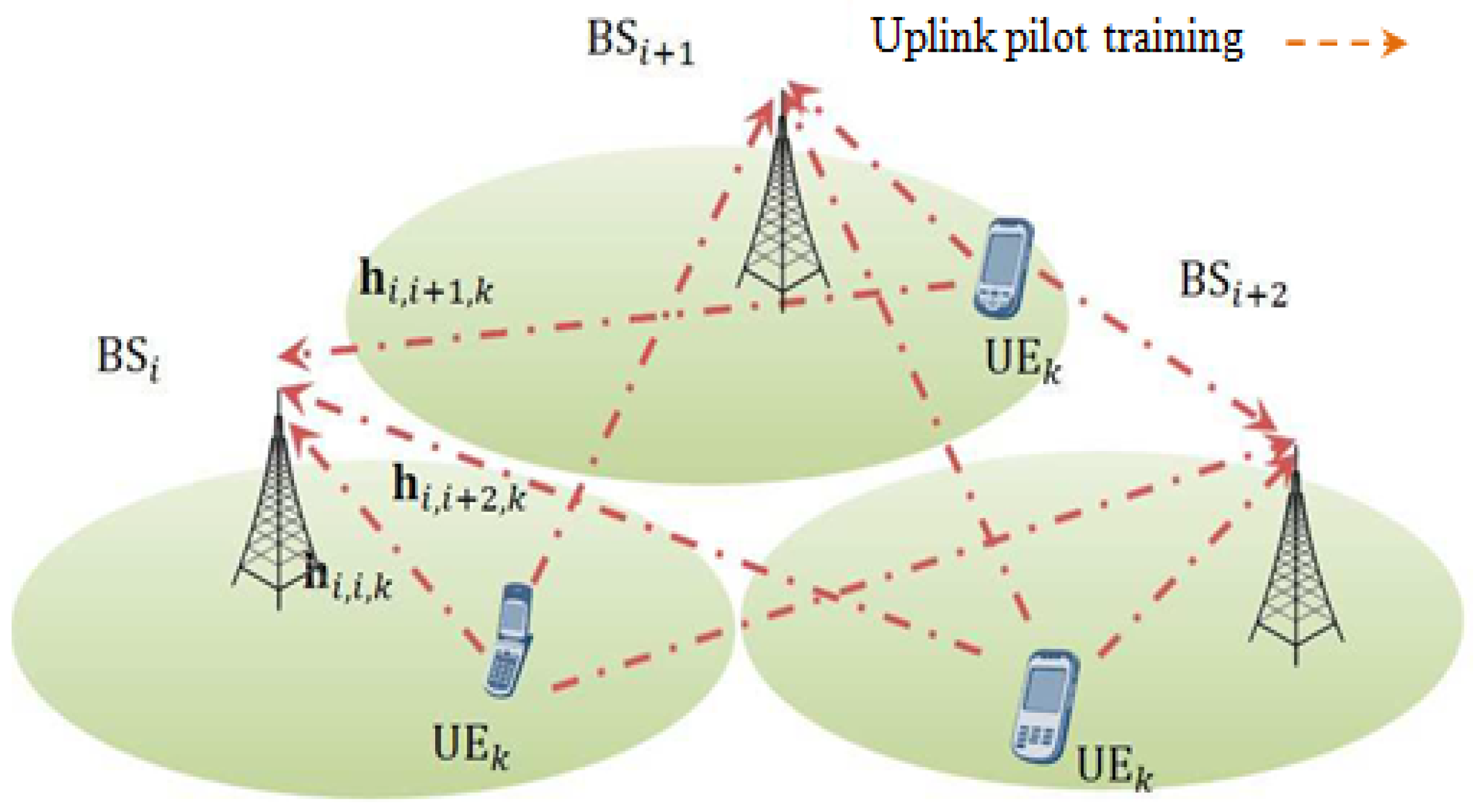
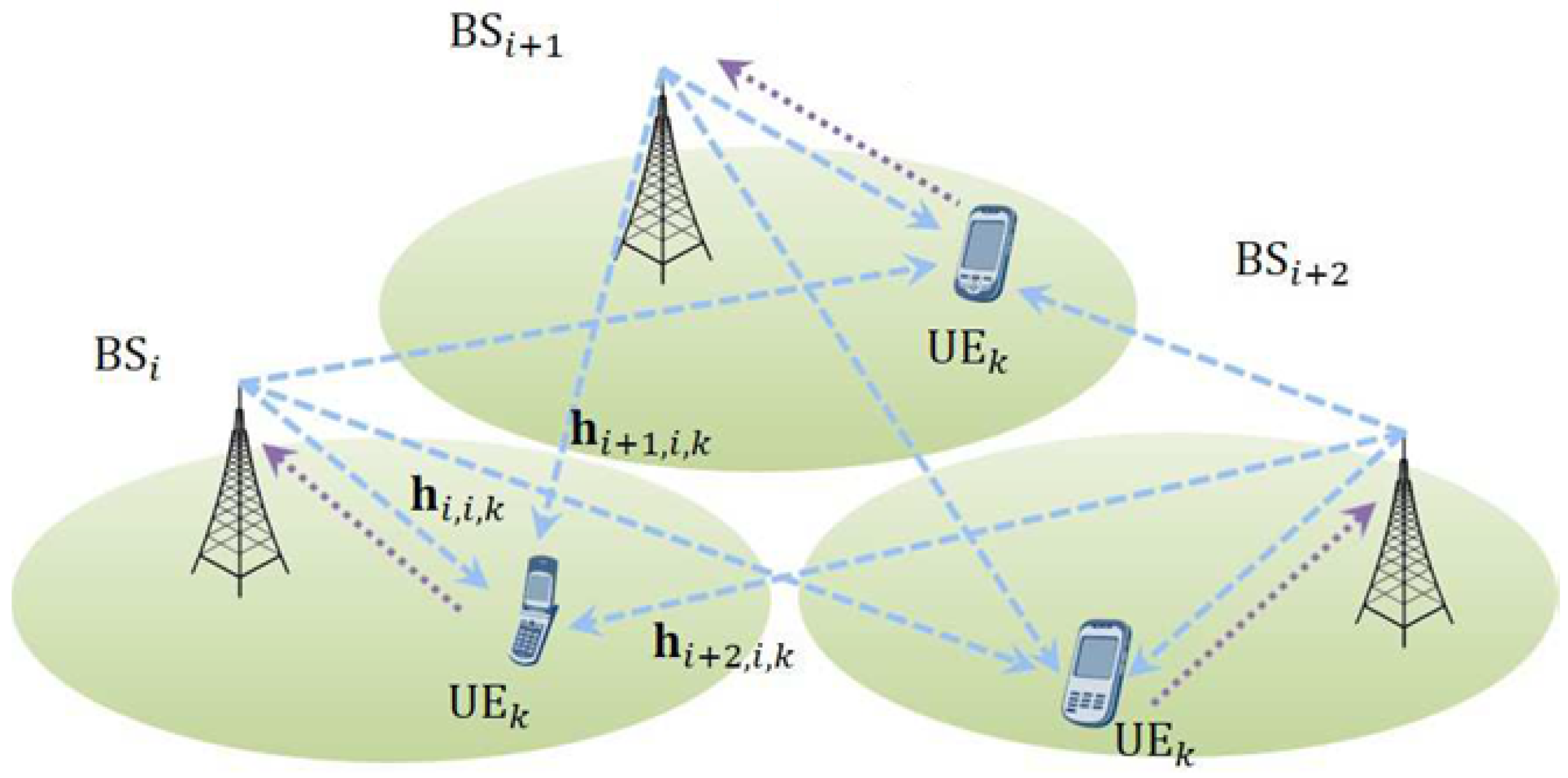
At the beginning of each coherence interval T_coh, the terminals transmit pilot sequences with length τ. Each mth antenna at base station in jth cell will receive a vector y_jm with length τ from kth user in ℓth cell as shown in Figure 1, where each BS received pilot sequence from its cell and other cells due to limited number of orthogonal pilot sequences that leads to problem of pilot contamination, then the received signal is defined by

$$y_{jm}={\displaystyle \sum _{\ell =1}^L{\displaystyle \sum _{k=1}^K\sqrt{p_u{\mathsf{\tau }\mathsf{\beta }}_{jk\ell }}{h}_{jk\ell }{\mathsf{\psi }}_{\ell k}+w_{jm}}},$$

(3)

where w_jm is the additive white Gaussian noise (AWGN) whose elements are i.i.d. with zero mean and variance σ²_w, so the noise vector at jth cell is defined by W_j which is a M × τ vector and W_j = [w_j1, w_j2,…, w_jm]. Y_j is the received signal vector with dimension M × τ, so the received vector is defined by Y_j = [y_j1, y_j2,…, y_jm], while the terms {(τ)^1/2ψ_jℓ} is the training sequence vector transmitted by kth user in ℓth cell where ψ_ℓ = [ψ_ℓ1, ψ_ℓ2,…, ψ_ℓk] with τ × K.

Then the received signal at BS is given by

$$Y_j=\sqrt{p_u\mathsf{\tau }}{\displaystyle \sum _{\ell =1}^L{\mathsf{\psi }}_{\ell }{G}_{j\ell }+W_j}.$$

(4)

After receiving the signal, the BS estimates the propagation channel matrix G using linear estimation theory such as MMSE estimator [23]. Each base station transmits a vector of message-bearing symbols through a precoding matrix which depends on estimation channel matrix Ĝ_jj, then linearly precoded these symbols. After that, the BS will move the precoded signal vector to all users. The estimated channel matrix for M × K propagation matrix G_jj between the M base station antennas of jth cell and the K terminals in the same jth cell is defined by Ĝ_jj which is obtained according to the following expression:

$${\widehat{G}}_{jj}=\sqrt{p_p}{\displaystyle \sum _{\ell =1}^L{G}_{j\ell }+V_j},$$

(5)

where V_j is the noise matrix with M × K elements which are AWGN with zero mean mutually uncorrelated, and uncorrelated with the propagation matrices, P_p is the pilot signal to noise ratio, and since M goes to infinity, the effects of noise will be vanished, as in the present work which it is defined as the average pilot transmitted power.

At the uplink communication phase, K users in each cell independently send data streams to their related base station. The base station at jth cell will receive M × 1 vectors including transmissions from all of the terminals in the L cells. Then the received signal vector at base station is defined by

$${\overline{r}}_j=\sqrt{p_p}{\displaystyle \sum _{\ell =1}^L{G}_{j\ell }{b}_{\ell }+z_j},$$

(6)

where b_ℓ is the K × 1vector of message-bearing symbols from the terminals of the ℓth cell, z_j is a vector of received noise whose components are AWGN with zero-mean, mutually uncorrelated and uncorrelated with the propagation matrices. The message-bearing signals are transmitted by the terminals and they are independent and distributed with zero-mean, unit-variance and complex Gaussian variables. The base station uses its estimated channel to perform linear detecting process such as MRC, ZF and MMSE detectors. By using the linear detector, the received signal is divided into streams by multiplying it with the linear detector matrix, which depends on the pseudo inverse of the propagation channel G. With maximum ratio combining (MRC) detector, the base station processes its received signal by multiplying it with the conjugate-transpose of the estimated channel. Let A be an K × M linear detector matrix which depends on the channel Ĝ and $r_j$ is the M × 1 received vectors, then

$$r_j=A\cdot {\overline{r}}_j,$$

(7)

where $A={\widehat{G}}_{jj}^H$.

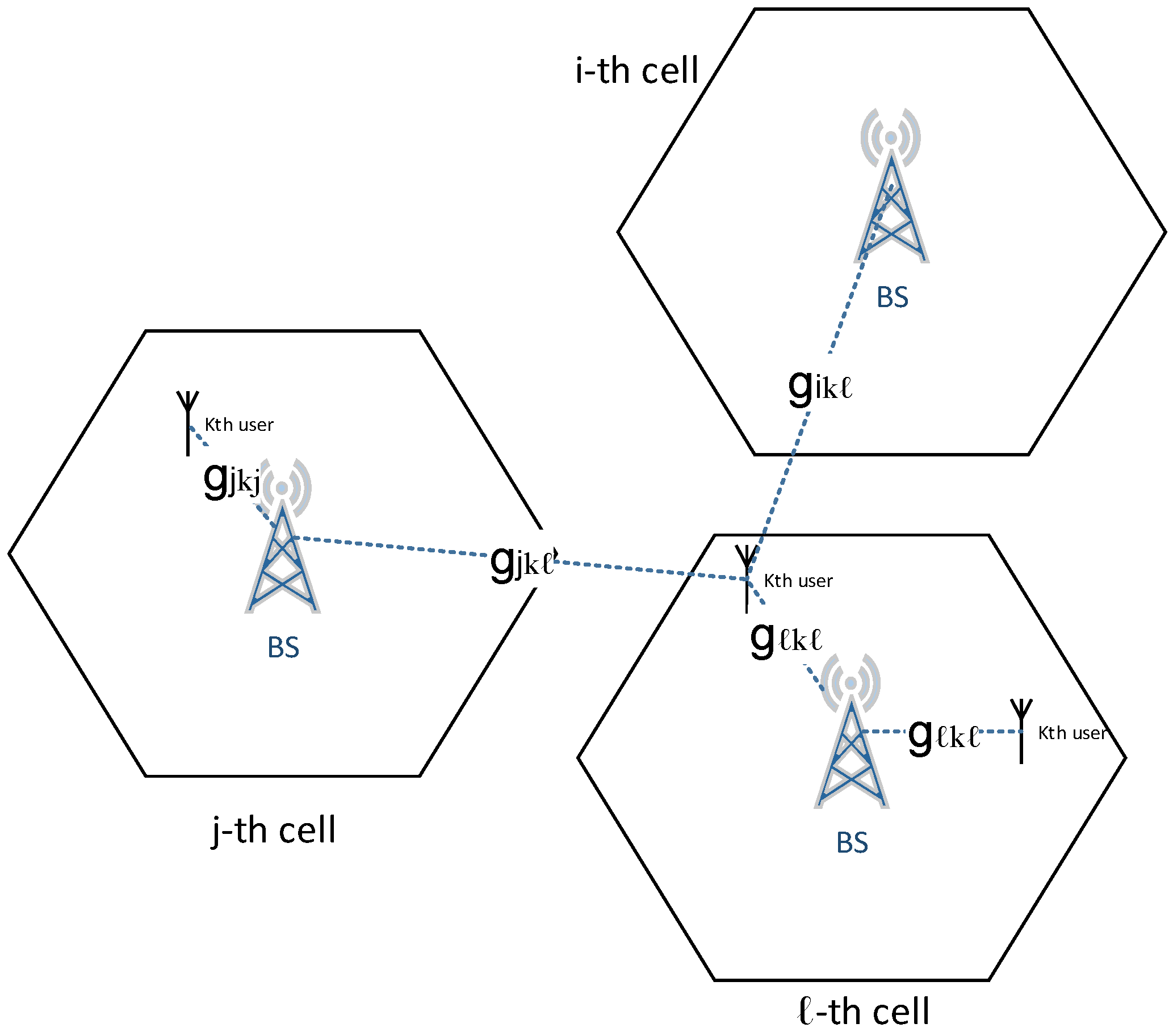
2.2. Downlink Communication Phase

Let s_jk be the symbol to be transmitted to the kth user with E {|s_jk|²} = 1. The BS uses the channel estimate to linearly precode the symbols, and then moves the precoded signal vector to all users. The K × 1 received signal vectors (Q_ℓ) at the K terminals in ℓth cell from base stations in other cells is given by

$$Q_{\ell }=\sqrt{p_d}{\displaystyle \sum _{j=1}^L{G}_{j\ell }^T{O}_j{s}_j+}{n}_{d\ell },$$

(8)

where O_j is the precoding matrix with M×K complex values of the jth BS, consequently O_j is selected to be as $p_d=E\left\{{\Vert \sqrt{p_d}{O}_j{s}_j\Vert }^2\right\}$, where E{||·||2}is the expected value of the Euclidean norm value and the transmit precoded signal is given by $\sqrt{p_d}{O}_j{s}_j$. “T” is the transpose operator and n_dℓ is the AWGN vector with variance σ²_n. Using the linear precoding method MRT, the precoding matrix is computed as in [24]

$$O_j=f_{MRT}{\widehat{G}}_{jj}^{*},$$

(9)

where f_MRT is the normalization constant chosen to satisfy the transmit power constraint at the BS and “*” is the complex conjugate.

Figure 2 explains the data transmissions at downlink broadcast channel from base station to their terminals where terminal with the same pilot sequence will interfere with users in other cells.

3. Massive MIMO Performance Gains

In this work, the performance of massive MIMO system will be measured under two main considerations: perfect and imperfect channel state information (CSI). After that, we will discuss how to measure the massive MIMO channel performance in terms of spatial multiplexing, spatial diversity and array gains.

Perfect channel state information means the base station has perfect knowledge about the propagation channel matrix G. The base station can use any linear detector to perform well i.e., (MRC, ZF…) as (M >> K). Theoretically, the singular value decomposition (SVD) of the channel matrix G would be taken in precoding and detecting process with removing the two unitary matrices, hence one data stream per singular value can be transmitted without creating any interference, i.e., the effect of non-orthogonal channel vectors from other cells. Channel capacity could be achieved in massive MIMO without pilot overhead effect on time coherence interval [25].

Practically, the channel matrix G has to be estimated at BS during the uplink training phase. If T_coh is the length of the coherence interval and τ be the number of symbols used for pilot sequences, all users concurrently transmit reciprocal orthogonal pilot sequences of length τ symbols. The channel state information (CSI) at the base station is a core component when trying to maximize network throughput. The only factor that remains limiting performance in massive MIMO is the inter-cell interference since when it is associated with the finite time existing to send pilot sequences, it makes the appreciated CSI at one BS “contaminated” by the CSI of users in adjacent cells, which is called pilot contamination effect. This phenomenon results from unavoidable re-use of reverse link pilot sequences by terminals in different cells. Clearly, in multi-cell massive MIMO system, as M tends to infinity, the downlink SINR (Υ_ℓk) of kth user at ℓth cell is proportional according to the following expression

$${\mathsf{{\rm Y}}}_{\ell k}\propto \frac{p_{dk\ell }{\mathsf{\beta }}_{\ell k\ell }^2}{{\displaystyle \sum _{\begin{array}{l}j=1\\ j\ne \ell \end{array}}^L{p}_{dkj}{\mathsf{\beta }}_{jk\ell }^2}},$$

(10)

where p_dk is the downlink transmit power delivered by BS to kth user in its cell. β_ℓℓ and β_jℓ are the direct and the cross gains respectively, which represent the effect of pilot contamination [12].

However, the mobility of users is closely related to the quality of the channel state information (CSI), which can be acquired at the BSs, high mobility implies low-quality of CSI. With multi-cell massive MIMO, base stations transmit the forward data symbols during the coherent time to their terminals depending on the uplink training sequences for channel estimations, but actually imperfect channel information may be obtained because of imperfect uplink training sequences channel estimation, delay in the acquisition protocols and user mobility. Because the coherence time of the MIMO channel inversely proportional with high user mobility, large channel imperfections will be as terminal mobility increases [19]. The channel model is suggested to represent the imperfect CSI by modeling the fading channel as

$$h_{\ell ,k}^m=\sqrt{X_{\ell ,k}^m}\left[\sqrt{\left(1-{\left({\mathsf{\tau }}_{\ell ,k}^m\right)}^2\right)}{h}_{\ell ,k}^m+{\mathsf{\tau }}_{\ell }^m{h}_{\ell ,k}^{~m}\right],$$

(11)

where $h_{\ell ,k}^m$ is the channel between the BS at mth cell and kth terminal in ℓth cell, $h_{\ell ,k}^{~m}$ is the channel estimation error. In this formula, the accuracy of channel request can be setting between the terminals in ℓth cell and BS in cell mth by setting ${\mathsf{\tau }}_{\ell }^m\in [0,1]$, which is the training sequences time interval and a small number on τ means low mobility and vice versa [26].

3.1. Spatial Diversity Gain

In wireless communication system, the received signal suffers from the effects of propagation environment. To achieve high link quality, special diversity techniques are used to improve the received signal quality through multipath propagation like MIMO system. The idea of diversity includes providing each terminal multiple copies of the transmitted signal. Therefore, the probability that one of the copies is not facing a deep fade effect rises. By growing the number of separated paths, the link probability also rises. Spatial diversity gain can be defined as the measurement of link reliability and the number of independent fading links as the diversity order. Massive MIMO system provides a large degree of freedom compared with the number of terminals, which means improving the channel reliability and the quality of received data. The link reliability is measured by the outage probability or the bit error rate. For Rayleigh fading channel the measurement of diversity depends on the degree of correlation between the fading coefficient random variables which they construct the massive MIMO channel matrix. Therefore, fewer correlations between channel coefficients lead to less fluctuation in the received signal, then link reliability can be expected. The diversity gain can limit the amount of variation in the received signal which can be computed by diversity measurement (D_div) as [27]

$$D_{div}(C)=\frac{{(trC)}^2}{tr(C^2)}.$$

(12)

From expression (12), it can be noted that a high value of diversity referring to lower fluctuation in the received signal, where C is the correlation matrix for i.i.d Rayleigh fading channel matrix of massive MIMO system. The diversity gain is calculated according to the diversity measurement, which is the product of the diversity measurement at the downlink side and uplink side in terms of the correlation matrix as shown below

$$D_{div}(C)=D_{div}(C)\times D_{div}(C_{UL}).$$

(13)

The benefit of diversity measurement at both channels is to decide which of the massive MIMO channel propagation matrix has stronger fading correlation or more diversity, the correlation matrix at the downlink side for massive MIMO channel can be written as

$$C_{DL}=E[G^{H}G].$$

(14)

While the correlation matrix for massive MIMO at the uplink side is

$$C_{UL}=E[G{G}^H].$$

(15)

3.1.1. Downlink Side

Let X be defined as the effective channel matrix at the transmit side, which includes the propagation channel matrix G_jj and the precoding matrix O_j. Here G_jℓ is the propagation channel matrix between the base stations in other cells and the kth terminals in ℓth cell where they are served by their BS, i.e., pilot contamination effects. Then, from Equation (8) the effective channel matrix can be written as

$$X=\sqrt{p_d}{\displaystyle \sum _{j=1}^L{G}_{j\ell }^T}{O}_j.$$

(16)

Now, using expressions (9), expression (16) can be rewritten as below

$$X=\sqrt{p_d}{\displaystyle \sum _{j=1}^L{G}_{j\ell }^T}{f}_{MRT}{\left[\sqrt{p_d}{\displaystyle \sum _{{\ell }^{\prime }=1}^L{G}_{j{\ell }^{\prime }}+V_{j1}}\right]}^{\ast }.$$

(17)

Diversity gain (G_div-DL) measured under imperfect CSI in terms of diversity measurement (D_div) at the downlink side is given by

$$G_{div-DL}={\mathrm{D}}_{div} (E[X^{H}X])=\frac{{(tr\hspace{0.17em}{C}_{DL})}^2}{tr(C_{DL}^2)}.$$

(18)

As M grows unlimited, only the products of identical quantities remain significant, i.e., the propagation matrices which appear in both of the bracketed expressions, and if the BS has a large number of antennas and the channels are i.i.d fast flat Rayleigh fading channels, then the channel vectors between the users and the BS become orthogonal. Massive MIMO channel vectors are regulated by the law of orthogonality, which is clarified in Theorem 1 below.

Theorem 1:

Let W = [w₁, w₂,…, w_M]^T and A = [a₁, a₂, …, a_M]^T are vectors whose elements are independent, identically distributed (i.i.d) random variables with zero mean and variance E[|w_i|²] = σ²_w and E[|a_i|²] = σ²_a for i=1, 2, …, M respectively. As a result from the law of large numbers, then the following will be obtained:

$$\frac{1}{M}{W}^{H}W\to {\mathsf{\sigma }}_w^2 \mathrm{and} \frac{1}{M}{W}^{H}A\to 0 \mathrm{as} M \to \infty$$

Now, if the conditions of the above theorem are satisfied for such as any vectors W and A are being any two distinct columns of G propagation matrix, then

$$\frac{1}{M}{G}_{j\ell 1}^H{G}_{j\ell 2}=D_{j\ell 1}^{1/2}{D}_{j\ell 2}^{1/2}\left(\frac{H_{j\ell 1}^H{H}_{j\ell 2}}{M}\right)\approx D,$$

(19)

where,

$$\frac{1}{M}{H}_{j\ell 1}^H{H}_{j\ell 2}=I_K{\delta }_{\ell 1\ell 2}\hspace{0.17em}\hspace{0.17em}\hspace{0.17em}as\hspace{0.17em}\hspace{0.17em}\hspace{0.17em}M\to \infty ,$$

(20)

where I_K is K × K identity matrix. Therefore, favorable propagation is attained with i.i.d random variables with zero mean and (M >> K). Hence, the diversity gain at downlink side can be written as

$$\begin{array}{ll}{G}_{div-DL}& ={\mathrm{D}}_{div} (E[X^{H}X])\\ & =M{f}_{MRT}{p}_p{p}_d{D}_{\ell \ell }+M{f}_{MRT}{p}_p{p}_d{\displaystyle \sum _{\begin{array}{l}j=1\\ j\ne \ell \end{array}}^L{D}_{j\ell }}\end{array}.$$

(21)

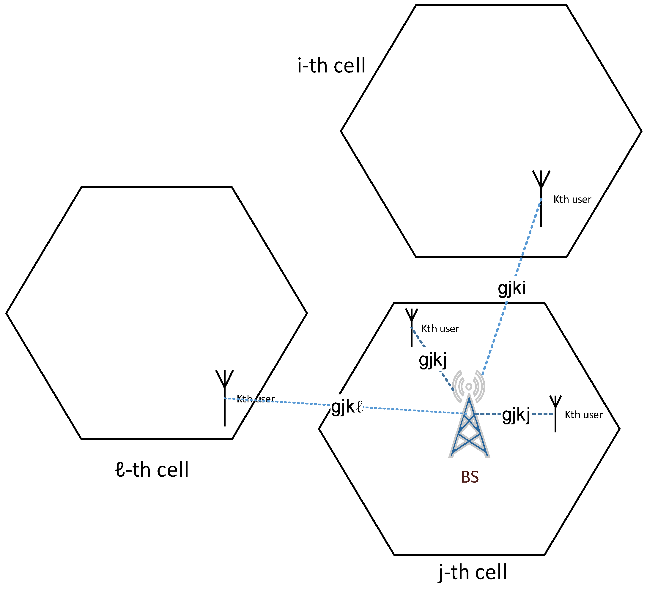
From expression (21), the first term represents the propagation channels between the users and BS in ℓth cell, while the second term represents propagation channels from base stations in other cells directed to their own K terminals interfering with the propagation channels from the base station in the ℓth cell to its K terminals. This interference due to the effect of pilot contamination is shown in Figure 3 below. With keeping the originality for M to grow with unlimited number, the final expression for diversity gain at downlink side is

$$G_{div-DL}={\mathrm{D}}_{div} (E[X^{H}X])=\frac{{\left(tr{D}_{\ell \ell }{D}_{j\ell }\right)}^2}{tr\left(D_{\ell \ell }^2{D}_{j\ell }^2\right)}.$$

(22)

3.1.2. Uplink Side

The M × 1 received vectors at the jth BS after applying the MRC detection at the BS is given by expression (7), then using expression (5) for channel estimation, so we have

$$r_j={\left[\sqrt{p_p}{\displaystyle \sum _{\ell =1}^L{G}_{j\ell }+V_{j1}}\right]}^H\left[\sqrt{p_u}{\displaystyle \sum _{{\ell }^{\prime }=1}^L{G}_{j{\ell }^{\prime }}{b}_{{\ell }^{\prime }}+z_j}\right].$$

(23)

Considering the properties of the correlation matrix for massive MIMO channel of the received signal vector r_j, the diversity gain at the uplink side can be obtained in terms of correlation matrix where the correlation matrix is

$$C_{UL}=E\left[r_j{r}_j^H\right].$$

(24)

Then the diversity gain (G_div-UL) is determined under imperfect CSI in terms of diversity measurement (D_div) at the uplink channel side as

$$G_{div-UL}={\mathrm{D}}_{div}E\left(\left[r_j{r}_j^H\right]\right).$$

(25)

For massive MIMO system, as M increases without limit, the effects of additive receiver noise and fast fading disappear, as well as intra-cell interference, then according to expressions (19) and (20) for channel orthogonality, the following is obtained

$$\begin{array}{ll}{G}_{div-UL}& ={\mathrm{D}}_{div}E\left(\left[r_j{r}_j^H\right]\right)\\ & =M{p}_p{p}_u{D}_{jj}+M{p}_p{p}_u{\displaystyle \sum _{\begin{array}{l}\ell =1\\ \ell \ne j\end{array}}^L{D}_{j\ell }}\end{array}.$$

(26)

From expression (26), the first term represents the propagation channels between the users and BS in jth cell, while the second term represents propagation channels from terminals in other cells which use the same pilot sequences interfering with the transmission from the kth terminal in the jth cell to its own base station in jth cell as shown in Figure 4 below. Then, the final expression for diversity gain at uplink side is

$$G_{div-UL}=D_{div}E\left(\left[r_j{r}_j^H\right]\right)=\frac{{\left(tr{D}_{jj}{D}_{j\ell }\right)}^2}{tr\left(D_{jj}^2{D}_{j\ell }^2\right)}.$$

(27)

As a result, expressions (22) and (27) are given for diversity gain at downlink and uplink channels respectively, which are the same expression, but in fact they have different statistical characteristics, where at the downlink side the transmission from the base station in any cell to its K terminals suffering interference from transmissions of the base stations in other cells to their own K terminals. While at the uplink side, the transmission from the terminal in any cell to its base station is suffering the interferences from the transmissions of terminals in the other cells to their base stations. These interferences are caused due to the pilot contamination.

At the downlink, BS uses the estimated channel to precode the transmit signals to users, while at the uplink side the signals transmitted from users can be decoded using the channel estimations. With massive MIMO systems, the number of base stations’ antennas is unlimited, so that the number of cells that use the same band frequencies are increased which causing high time delay for the CSI between the uplink training sequence and downlink data transmission which increase the diversity gain loss [13].

The total diversity gain is the product of the uplink and downlink diversity gains, it can be written as

$$G_{div-TL}=G_{div-DL}\cdot \hspace{0.17em}{G}_{div-UL}.$$

(28)

This expression quantifies the degree of fluctuation in the received power signal and how much the uplink and the downlink side be affected by this fluctuation. The number of independent fading link offers by massive MIMO is equal to the number of transmit antennas and the number of received antennas, which is named the diversity order (θ_ord). A massive MIMO channel with M antennas at the downlink side and K antennas at the receiving side has diversity order of

$${\mathsf{\theta }}_{ord}=M\times K.$$

(29)

3.2. Array Gain

One of the main important advantages of massive MIMO technology is to increase the power efficiency compared to MIMO system. A system with very large antenna arrays at base station in which each antenna has a small physical size, such system requires a small amount of transmit power. Therefore, the power radiated by terminals could be made inversely related to the square-root of the number of base station antennas with no reduction in performance if the base station has imperfect channel estimation, while in the case of perfect estimation the radiated power could be made inversely related to the number of antennas. The reduction of terminals’ transmit power will drain their batteries slower on the multi-access channel while reducing the emitted RF power would help in cutting the power consumption of the base station on the broadcast channel [24]. Another benefit of a large number of antennas is the ability to increase the tolerance to noise as well as the interference power, hence improving the signal to noise plus interference ratio (SINR) which means that interference can be reduced in massive MIMO systems by exploiting the spatial dimension to increase the separation between users.

In general, an array gain is defined as the ratio between the received power in massive MIMO ($P_{re}^{Massive\hspace{0.17em}MIMO}$) and the received power in MIMO system ($P_{re}^{\hspace{0.17em}MIMO}$) [28], which is given by

$$G_{array}=\frac{P_{re}^{Massive\hspace{0.17em}MIMO}}{P_{re}^{MIMO}},$$

(30)

with multi-cell massive MIMO system under imperfect conditions, the radiated power required by terminals is $p_u\propto 1/\sqrt{M}$, where p_u is the transmitted power by terminals and M is the number of BS’s antennas, while under perfect conditions, the radiated power required by terminals is $p_u\propto 1/M$ [29]. With massive MIMO, a system with an unlimited number of antennas at the base station, the transmitter must have knowledge of the channel state information to exploit the array gain. In this paper, two cases of CSI are considered in order to derive an expression for array gain in multi-cell massive MIMO system, then a formula will be derived for the received signal power at terminals in the downlink channel.

3.2.1. Array Gain under Perfect CSI

With perfect CSI, the propagation channel G is known by the base station. At the downlink side, the received signal for k terminals in ℓth cell from their base station is given by expression (8), here it is assumed that each BS has its transmit power to their K terminals, which will be defined as [30]

$$Q_{\ell }={\displaystyle \sum _{j=1}^L\sqrt{p_{dj}}{G}_{j\ell }^T{O}_j{s}_j+n_{d\ell }},$$

(31)

Let $U_j=\sqrt{p_{dj}}{O}_j{s}_j$ is the pre-coded transmit vector to K terminals in ℓth cell, where p_dj is the diagonal matrix and consists of the downlink transmit power for K terminals of BS, where P_dj=diag(p_d1j, p_d2j, …, p_dKj) and the propagation channel matrix G is being as in expression (2). Then the total transmit power at jth cell is

$$P_{Tj}=E\left[{\Vert \hspace{0.17em}{U}_j\Vert }^2\right]=tr(O_j^H{O}_j{P}_{dj})=tr(P_{dj}),$$

(32)

For massive MIMO system, as M increases without limit, the effects of additive receiver noise and fast fading disappear. With perfect CSI, BS knows the propagation channel matrix G, the effect of the interference between users in the same cell is disappeared. However, still there is the interference among the users from other cells, and with perfect CSI this effect also can be eliminated supposing the system behaves as a single cell [31]. According to expressions (19) and (20), the channel vectors between the users and the BS become orthogonal, as M grows unlimited then the received signal power under perfect CSI is defined as

$$\begin{array}{ll}{P}_{re}^{Massive\hspace{0.17em}MIMO}& =E\left[{\Vert \hspace{0.17em}{Q}_{\ell }\Vert }^2|G\right]=M\left({\displaystyle \sum _{j=1}^L{P}_{dj}{D}_{j\ell }}\right)\\ & =M\left(P_{d\ell }{D}_{\ell \ell }+{\displaystyle \sum _{j\ne \ell }^L{P}_{dj}{D}_{j\ell }}\right)\end{array},$$

(33)

where D_jℓ is a K × K diagonal matrix whose diagonal elements are [D_jℓ]_kk = β_jkℓ. The first term in expression (33) represents the propagation channels between the users and the base station in ℓth cell, while the second term represents the propagation channels from the base stations in other cells to their users interfering with propagation channels between the users and the base station in ℓth cell.

Finally, as M→∞ (the case with massive MIMO) under perfect CSI, the effect of interference can be eliminated and the above expression will be

$$P_{re}^{Massive\hspace{0.17em}MIMO}=M\hspace{0.17em}tr(P_{d\ell }{D}_{\ell \ell }).$$

(34)

This expression is the received power in ℓth cell for massive MIMO regime. According to array gain definition, which is described in expression (30), the received power for MIMO system is given as

$$P_{re}^{MIMO}=tr(P_{\overline{d}}\Lambda ),$$

(35)

Where $P_{\overline{d}}$ is the diagonal matrix of the transmit power assigned to each data stream in MIMO and Λ is the diagonal matrix for the Eigen value of the propagation matrix H in MIMO system. Then the array gain can be given according to expression (30) with respect to massive MIMO under perfect CSI as

$$G_{Array}=\frac{P_{re}^{Massive\hspace{0.17em}MIMO}}{P_{re}^{MIMO}}=\frac{M\hspace{0.17em}tr(P_{d\ell }{D}_{\ell \ell })}{tr(P_{\overline{d}}\Lambda )}.$$

(36)

Massive MIMO technology enhances the system performance through array gain by increasing the number of antennas at base station with an unlimited number of antennas M.

3.2.2. Array Gain under Imperfect CSI

Practically, with multi-cell massive MIMO system, the propagation channel matrix G must be estimated at the base station through sending uplink pilot sequences from users to their base station. Because of the limitation in channel coherence interval, the number of orthogonal pilot sequences is limited also, as the number of antennas in base station increases with unlimited number, the number of served users increases also in each cell, hence the pilot sequences must be reused in other cells [32]. The reuse method is the main problem that causes the pilot contamination which affects the system performance through the error in channel estimation where the BS uses this estimation to build the precoding matrix for sending data to its users in downlink channel and this error increases the CSI delay, which is between the uplink training sequences and the downlink data for its users [13]. Under imperfect CSI, the array gain is computed according to the average received power, using expression (31) and with MRT precoding method (9) and substitute expression (5) in expression (9), the final expression for received vector to K terminals at ℓth cell is given by

$$Q_{\ell }=f_{MRT}{\displaystyle \sum _{j=1}^L\sqrt{p_{dj}}{G}_{j\ell }^T{\left[\sqrt{p_p}{\displaystyle \sum _{{\ell }^{\prime }=1}^L{G}_{j{\ell }^{\prime }}+V_{j1}}\right]}^{*}{s}_j+n_{d\ell }}.$$

(37)

The average received power under imperfect CSI is defined as

$$P_{re}^{Massive\hspace{0.17em}MIMO}=E\left[E\left[{\Vert \hspace{0.17em}{Q}_{\ell }\Vert }^2|\widehat{G}\right]\right].$$

(38)

In massive MIMO, as M increases without limit, the effects of additive received noise and fast fading disappear, as well as intra-cell interference, and according to expressions (19) and (20) for channel orthogonality we have

$$\begin{array}{ll}{P}_{re}^{Massive\hspace{0.17em}MIMO}& =E\left[E\left[{\Vert \hspace{0.17em}{Q}_{\ell }\Vert }^2|\widehat{G}\right]\right]\\ & =M\hspace{0.17em}{p}_{p}tr\left(P_{d\ell }{D}_{\ell \ell }+{\displaystyle \sum _{j\ne \ell }^L{P}_{dj}{D}_{j\ell }}\right)\end{array},$$

then,

$$P_{re}^{Massive\hspace{0.17em}MIMO}=M\hspace{0.17em}{p}_{p}tr\left(P_{d\ell }{D}_{\ell \ell }\right)+M\hspace{0.17em}{p}_p{\displaystyle \sum _{j\ne \ell }^L{P}_{dj}{D}_{j\ell }},$$

(39)

with imperfect CSI, the average received power for MIMO system is given as

$$P_{re}^{\hspace{0.17em}MIMO}=tr(P_{\overline{d}}{D}_{diag}),$$

(40)

where $P_{\overline{d}}$ is the diagonal matrix of the transmit power assigned to each data stream in MIMO and D_diag is the diagonal matrix for the Eigen value of the transmitted fading correlation matrix R_TX in MIMO system. Then the array gain can be given according to expression (30) with respect to massive MIMO under imperfect CSI follows

$$G_{array}=\frac{M\hspace{0.17em}{p}_{p}tr\left(P_{d\ell }{D}_{\ell \ell }\right)+M\hspace{0.17em}{p}_p{\displaystyle \sum _{j\ne \ell }^L{P}_{dj}{D}_{j\ell }}}{tr(P_{\overline{d}}{D}_{diag})}.$$

(41)

3.3. Spatial Multiplexing Gain

One of the main features of massive MIMO system is the ability to transmit multiple independent data streams in parallel at the same time and bandwidth, which offers a linear increasing in the data rate through the spatial multiplexing. Under suitable channel condition such as rich scattering, the receiver can decompose data streams. The need for multimedia services is rapidly increased, thus the capacity of wireless communication has to be increased in order to guarantee the quality of service requirements for mobile application. Therefore, wireless cellular networks are continuously developing to reach the user's demand for high data rate. Massive MIMO system is the key technology for high data throughput due to improve the spectral efficiency, which is necessary for increasing the channel capacity. Here, we consider the practical case where massive MIMO channel suffers from the effect of inter-cell interference in multi-cell massive MIMO system due to pilot contamination.

3.3.1. Multiplexing Gain under Perfect CSI

With perfect CSI, there is no need to pilot sequences received from users to make a channel estimation because the base station (transceiver) knows the propagation channel matrix G of massive MIMO system, and the precoding matrix is built on propagation channel matrix G. Users will receive the desirable data transmission from their BS without interfering with other users from other cells. It is assumed that the system is behaving as a single cell.

Considering the expression (31) for receiving data at downlink phase, and with perfect CSI, the precoding matrix is O_j = G* under MRT precoding method [3], and using the key concept for massive MIMO system on orthogonality when the number of antennas grows to infinity and using expressions (19) and (20), then

$$Q_{\ell }=M\hspace{0.17em}\sqrt{p_{d\ell }}{D}_{\ell \ell }{s}_{\ell }+M{\displaystyle \sum _{j=1}^L\sqrt{p_{dj}}{D}_{j\ell }{s}_j}+n_{d\ell },$$

(42)

with perfect CSI, the base station knows the propagation channel matrix, so it is assumed that the system behaves as a single cell. There is no interference between cells and the received signal vector for kth user is expressed as expression (31). The signal to noise ratio SNR for kth user in ℓth cell can be obtained as follows:

$$SN{R}_{k\ell }=\frac{M{p}_{d\ell k}{\mathsf{\beta }}_{\ell k\ell }^2}{{\mathsf{\sigma }}^2},$$

(43)

where σ² is the noise variance for the uncorrelated received noise. Then, the achievable rate for kth user in ℓth cell and achievable sum rate is given as

$$\begin{array}{l}{R}_{\ell k}={\log }_2(1+SN{R}_{k\ell })\\ R_{\ell }={\displaystyle \sum _{k=1}^K{R}_{\ell k}}\end{array},$$

(44)

Multiplexing gain under perfect CSI is defined as the deviation of the achievable sum rate as a function of transmitting power [33],

$$G_{MUX}^{perf.CSI}=\frac{d{R}_{\ell }}{d{\log }_2{p}_d}\hspace{0.17em}=\frac{d}{d{\log }_2{p}_d}{\displaystyle \sum _{k=1}^K{\log }_2\left(1+\frac{M{p}_{d\ell k}{\mathsf{\beta }}_{\ell k\ell }^2}{{\mathsf{\sigma }}^2}\right)},$$

(45)

$$G_{MUX}^{perf.CSI}={\displaystyle \sum _{k=1}^K\frac{M{\mathsf{\beta }}_{\ell k\ell }^2}{{\mathsf{\sigma }}^2+M{p}_{d\ell k}{\mathsf{\beta }}_{\ell k\ell }^2}},$$

(46)

with massive MIMO system, the number of base station antennas increases with unlimited number, then the above expression becomes

$$G_{MUX}^{perf.CSI}={\displaystyle \sum _{k=1}^K\frac{{\mathsf{\beta }}_{\ell k\ell }^2}{p_{d\ell k}{\mathsf{\beta }}_{\ell k\ell }^2}}={\displaystyle \sum _{k=1}^K\frac{1}{p_{d\ell k}}}=tr{(p_{d\ell })}^{-1}.$$

(47)

3.3.2. Multiplexing Gain under Imperfect CSI

In order to use the advantages that massive MU-MIMO can offer, accurate channel state information (CSI) is required at the BS. The impact of up-link training is significantly appearing in multi-cell system due to the same band of frequencies, which is shared by a multiplicity of cells. If each cell is serving the maximum number of terminals, then the pilot signals received by a base station are contaminated by pilots transmitted by terminals in other cells. Therefore, the user in the jth cell for example receives signal from its base station and from other base stations. If q_jk is the received signal for kth user, then

$$q_{jk}=\sqrt{p_{dj}{\mathsf{\beta }}_{jkj}}{h}_{jkj}{o}_j{s}_{jk}+{\displaystyle \sum _{\ell \ne j}\sqrt{p_{d\ell }{\mathsf{\beta }}_{\ell kj}}\hspace{0.17em}{h}_{\ell kj}}{o}_{\ell }{s}_{\ell k}+n_j.$$

(48)

The first term in the above expression represents the desired received signal while the second term reflects the effect of inter-cell interference. Pilot contamination affects system performance parameters such as achievable sum rate or spectral efficiency, channel capacity, received signal to interference plus noise and so on. In [34], the authors proposed a new detection method and derived a formula for signal to interference plus noise ratio (SINR) and spectral efficiency (SE), then calculated optimal number of terminals to achieve better performance is in term of achievable rate (R).

Many researches discuss how to mitigate the effect of polluted signals by modifying either the precoding methods which use at the forward channel or the discovery methods which is used at the reverse channel [35]. Now, let consider the received signal vector which is described previously in expression (31), and substitute expressions (5) and (9) in expression (31), the following will be obtained,

$$Q_{\ell }=f_{MRT}{\displaystyle \sum _{j=1}^L\sqrt{p_{dj}}}{G}_{j\ell }^T{\left[\sqrt{p_p}{\displaystyle \sum _{{\ell }^{\prime }=1}^L{G}_{j{\ell }^{\prime }}+V_{j1}}\right]}^{*}{s}_j+n_{d\ell }.$$

(49)

Since the number of base station’s antennas increases unlimitedly, the effect of intra-cell interference will vanish, while the effect of inter-cell interference still affects system performance. Using expressions (19) and (20) which is the key property of large MIMO system, then expression (49) will become

$$Q_{\ell }=M{f}_{MRT}\sqrt{p_p}\sqrt{p_{d\ell }}{D}_{\ell \ell }{s}_{\ell }+M{f}_{MRT}\sqrt{p_p}{\displaystyle \sum _{j\ne \ell }^L\sqrt{p_{dj}}}{D}_{j\ell }{s}_j+{\overline{n}}_{d\ell },$$

(50)

where ${\overline{n}}_{d\ell }$ is uncorrelated received AWGN noise with variance σ²_n. The received signal for kth user in ℓth cell is given by

$$Q_{\ell k}=M{f}_{MRT}\sqrt{p_p}\sqrt{p_{d\ell k}}{\mathsf{\beta }}_{\ell k\ell }{s}_{\ell k}+M{f}_{MRT}\sqrt{p_p}{\displaystyle \sum _{j\ne \ell }^L\sqrt{p_{djk}}}{\mathsf{\beta }}_{jk\ell }{s}_{jk}+{\overline{n}}_{d\ell }.$$

(51)

The first term is for the kth user in ℓth cell receives the transmitted data from its BS in cell, while the second term is for the effect of pilot contamination on the received data to kth cell user in ℓth cell, which interferes with the sending of data from other BSs to their users in other cells. As a result, the received SINR (Υ_ℓk) for kth user in ℓth cell is given by

$${\mathsf{{\rm Y}}}_{\ell k}=\frac{M{f}_{MRT}{p}_p{p}_{d\ell k}{\mathsf{\beta }}_{\ell k\ell }^2}{M{f}_{MRT}{p}_p{\displaystyle \sum _{j\ne \ell }^L{p}_{djk}{\mathsf{\beta }}_{jk\ell }^2+{\mathsf{\sigma }}_n^2}}.$$

(52)

Let T_coh be the length of coherence interval and τ be the number of symbols used for pilots, the achievable rate of the kth user within the multi-cell system and the effect of interference due to pilot contamination is given by

$$R_{\ell k}=\left(\frac{T_{coh}-\mathsf{\tau }}{T_{coh}}\right){\log }_2(1+{\mathsf{{\rm Y}}}_{\ell k}).$$

(53)

The term (T_coh − τ/T_coh)represents the pilot overhead, which is the ratio of the time needed in sending data to the coherence interval.

Then, the achievable sum rate for ℓth cell in multi-cell system under imperfect CSI is given by

$$R_{\ell }={\displaystyle \sum _{k=1}^K{R}_{\ell k}={\displaystyle \sum _{k=1}^K\left(\frac{T_{coh}-\mathsf{\tau }}{T_{coh}}\right)}}{\log }_2(1+{\mathsf{{\rm Y}}}_{\ell k}).$$

(54)

Multiplexing Gain under imperfect CSI is defined as the deviation of the average achievable sum rate as a function of the logarithmic transmit power [33]

$$G_{MUX}^{imperf.CSI}=\frac{dE(R_{\ell })}{d{\log }_2{p}_d}=\frac{d}{d{\log }_2{p}_d}{\displaystyle \sum _{k=1}^{K}E\left(\left(\frac{T_{coh}-\mathsf{\tau }}{T_{coh}}\right){\log }_2\left(1+\frac{M{f}_{MRT}{p}_p{p}_{d\ell k}{\mathsf{\beta }}_{\ell k\ell }^2}{M{f}_{MRT}{p}_p{\displaystyle \sum _{j\ne \ell }^L{p}_{djk}{\beta }_{jk\ell }^2+{\mathsf{\sigma }}_n^2}}\right)\right)}.$$

(55)

For massive MIMO system as the number of base station antennas M increases without limitation, the effects of received noise and fast fading are eliminated, just the effect of inter-cell interference remains due to the imperfect channel estimation, then the multiplexing gain can be given as

$$\begin{array}{l}{G}_{MUX}^{imperf.CSI}=\frac{d}{d{\log }_2{p}_d}{\displaystyle \sum _{k=1}^{K}E\left(\left(1-\frac{\mathsf{\tau }}{T_{coh}}\right){\log }_2\left(1+\frac{p_{d\ell k}{\mathsf{\beta }}_{\ell k\ell }^2}{{\displaystyle \sum _{j\ne \ell }^L{p}_{djk}{\mathsf{\beta }}_{jk\ell }^2}}\right)\right)}\\ \hspace{0.17em}{G}_{MUX}^{imperf.CSI}=\left(1-\frac{\tau }{T_{coh}}\right)\frac{tr(D_{\ell \ell }^2)\left[tr(p_{dj})-tr(p_{d\ell })\right]}{{\displaystyle \sum _{j\ne \ell }^L\left[tr{(p_{dj}{D}_{j\ell })}^2+tr(p_{d\ell }{D}_{\ell \ell }^2)tr(p_{dj})\right]}}\end{array}.$$

(56)

The detailed derivative of expression (56) can be shown in Appendix A. Expression (56) represents the multiplexing gain under the effect of undesirable interference between cells due to pilot contamination which is in term of the undesirable signal power from neighbor cells. All these are because of the BS in ℓth cell suffers from delay in channel estimation between the uplink pilot sequences during the training phase and data transmission in downlink phase. In addition, error channel estimation that all affect precoding matrix and this is why the transmission signals from other BSs to their users interfere with the received signal of kth user in ℓth cell from its BS.

4. Performance Tradeoffs Analysis

Practically, it is impossible to maximize all performance gains at the same time in massive MIMO system due to the effect of pilot contamination and also these gains are maximized by different transmit power distributions. In this section, two types of performance tradeoffs will be discussed among these gains under imperfect CSI.

4.1. Array 2Gain vs. Spatial Multiplexing Gain Tradeoff

A system consists of a large number of antennas can improve both energy efficiency and spectral efficiency significantly. However, increasing the achievable rate is associated with increasing the power which includes the radiated power and the circuit power and hence decreasing the energy efficiency. Therefore, to maximize one gain the other must keep with limited region. Energy efficiency is defined as the achievable sum rate divided by the power expended measured in Joules per used channel, while the spectral efficiency is defined as the achievable sum rate per unit of bandwidth.

In [36], the authors designed a macro-cellular large scale antenna system in order to maximize the total forward link energy efficiency, however the power consumed at ℓth cell is expressed as

$$P_{consumed}=P_{RF\ell }\left(1-\frac{\tau }{T_{coh}}\right)/2+P_{cct\ell },$$

(57)

where P_RFℓ is the RF power of base station in ℓth cell and it is weighted by $(1-\frac{\mathsf{\tau }}{T_{coh}})/2$ because downlink activities take half of the coherence interval. RF power can be defined in terms of total transmit power with RF efficiency (ε_RF), $R_{RF\ell }=\frac{1}{{\epsilon }_{RF}}{p}_{d\ell }$, where $p_{d\ell }={\displaystyle \sum _{k=1}^K{p}_{d\ell k}}$ and $P_{cct\ell }=M{p}_{cct\ell }$ is the internal circuit power which is expended on massive MIMO system due to critical computations and other activities such as analog electronics and A/D and D/A conversions, P_cctℓ is internal circuit power of each antenna. To calculate the energy efficiency (η_e,ℓ) at ℓth cell downlink side and using expressions (52) and (54) for channel capacity then we have

$${\mathsf{\eta }}_{e,\ell }=\frac{{\displaystyle \sum _{k=1}^K{R}_{\ell k}}}{P_{consumed}},$$

(58)

$$\begin{array}{l}{\mathsf{\eta }}_{e,\ell }=\frac{\left(1-\frac{\mathsf{\tau }}{T_{coh}}\right){\displaystyle \sum _{k=1}^K{\log }_2(1+{\mathsf{{\rm Y}}}_{\ell k})}}{\frac{1}{{\mathsf{\epsilon }}_{RF}}{p}_{d\ell }\left(1-\frac{\mathsf{\tau }}{T_{coh}}\right)/2+P_{cct\ell }}\\ {\mathsf{\eta }}_{e,\ell }=\frac{\left(1-\frac{\mathsf{\tau }}{T_{coh}}\right){\displaystyle \sum _{k=1}^K{\log }_2\left(1+\frac{M{f}_{MRT}{p}_p{p}_{d\ell k}{\mathsf{\beta }}_{\ell k\ell }^2}{M{f}_{MRT}{p}_p{\displaystyle \sum _{j\ne \ell }^L{p}_{djk}{\mathsf{\beta }}_{jk\ell }^2+{\mathsf{\sigma }}_n^2}}\right)}}{\frac{1}{{\mathsf{\epsilon }}_{RF}}{p}_{d\ell }\left(1-\frac{\mathsf{\tau }}{T_{coh}}\right)/2+P_{cct\ell }}\end{array}.$$

(59)

Using the expression of SINR in expression (52), then the spectral efficiency for ℓth cell (η_s,ℓ) in downlink massive MIMO system is written as

$${\mathsf{\eta }}_{s,\ell }=\left(1-\frac{\mathsf{\tau }}{T_{coh}}\right){\displaystyle \sum _{k=1}^K{\log }_2\left(1+\frac{M{f}_{MRT}{p}_p{p}_{d\ell k}{\mathsf{\beta }}_{\ell k\ell }^2}{M{f}_{MRT}{p}_p{\displaystyle \sum _{j\ne \ell }^L{p}_{djk}{\mathsf{\beta }}_{jk\ell }^2+{\mathsf{\sigma }}_n^2}}\right)}.$$

(60)

Assuming all users are sharing the same constant bandwidth, so the bandwidth is ignored in this work. To study the tradeoff between energy efficiency and spectral efficiency, the expression mentioned in [16] is considered, where the authors discussed the tradeoff under two cases: perfect CSI and no CSI with single user and multi-user as follows

$$\frac{d{\mathsf{\eta }}_{e,\ell }}{d{\mathsf{\eta }}_{s,\ell }}=\frac{{\displaystyle \sum _{k=1}^K\frac{\partial {\mathsf{\eta }}_{e,\ell }}{\partial p_{d\ell k}}}d{p}_{d\ell k}}{{\displaystyle \sum _{k=1}^K\frac{\partial {\mathsf{\eta }}_{s,\ell }}{\partial p_{d\ell k}}}d{p}_{d\ell k}}.$$

(61)

In the present work, the tradeoff in multi-cell massive MIMO system is discussed under imperfect CSI taking into account the effect of coherent interference, i.e., pilot contamination effect. Each performance gain needs different transmit power to reach the maximum value, so the partial derivative is taken with respect to transmit power for each user in the cell. Then the above expression (61) will be

$$\frac{d{\mathsf{\eta }}_{e,\ell }}{d{\mathsf{\eta }}_{s,\ell }}=\frac{\left(1-\frac{{\mathsf{\tau }}_p}{T_{coh}}\right){\displaystyle \sum _{k=1}^K\frac{\frac{\partial {\mathsf{\eta }}_{s,\ell }}{\partial p_{d\ell k}}\left(\frac{1}{{\mathsf{\epsilon }}_{RF}}{\displaystyle \sum _{k=1}^K{p}_{d\ell k}\left(1-\frac{{\mathsf{\tau }}_p}{T_{coh}}\right)/2+P_{cct\ell }}\right)-\frac{{\mathsf{\eta }}_{s,\ell }}{{\mathsf{\epsilon }}_{RF}}\left(1-\frac{{\mathsf{\tau }}_p}{T_{coh}}\right)/2}{{\left(\frac{1}{{\mathsf{\epsilon }}_{RF}}{\displaystyle \sum _{k=1}^K{p}_{d\ell k}\left(1-\frac{{\mathsf{\tau }}_p}{T_{coh}}\right)/2+P_{cct\ell }}\right)}^2}}\hspace{0.17em}d{p}_{d\ell k}}{{\displaystyle \sum _{k=1}^K\frac{\partial {\mathsf{\eta }}_{s,\ell }}{\partial p_{d\ell k}}}d{p}_{d\ell k}}.$$

(62)

To discuss the relation between energy and spectral efficiencies, if the spectral efficiency approaches zero, the SINR will be also zero. Expression (62) is inversely proportional to total power consumed under the effect of pilot overhead, and then the following is obtained

$$\underset{p_{dk}\to 0}{{\displaystyle \lim }}\frac{d{\mathsf{\eta }}_{e,\ell }}{d{\mathsf{\eta }}_{s,\ell }}=\frac{\left(1-\frac{{\mathsf{\tau }}_p}{T_{coh}}\right)}{P_{cct\ell }}.$$

(63)

Theorem 2:

At high SNR regime, the channel capacity increases with M transmit, K received antennas and i.i.d Rayleigh faded gains between each antenna pair, would be increased by the factor min $\{M,K,\frac{T_{coh}}{2}\}$ which is the total number of degree of freedom.

Using the principle of Theorem 2 above, and for the massive MIMO multi-cell system under imperfect CSI with high SNR regime, the capacity is given by

$$R_{rate}=\min \{M,K,\frac{Tcoh}{2}\}\left(1-\frac{\tau }{T_{coh}}\right){\displaystyle \sum _{k=1}^K\log (SINR)},$$

(64)

min $\{M,K,\frac{T_{coh}}{2}\}$ represents parallel spatial channels, while $\frac{T_{coh}}{2}$ is for one data transmission phase, i.e., downlink or uplink data transmission [37].

Corollary 1:

As the number of antennas approaches infinity in massive MIMO, the spectral efficiency will increase, then SINR expression (Υ_ℓk) will be written as

$$\underset{M\to \infty }{\lim }{\mathsf{{\rm Y}}}_{\ell k}=\underset{M\to \infty }{\lim }\frac{M{f}_{MRT}{p}_p{p}_{d\ell k}{\mathsf{\beta }}_{\ell k\ell }^2}{M{f}_{MRT}{p}_p{\displaystyle \sum _{j\ne \ell }^L{p}_{djk}{\mathsf{\beta }}_{jk\ell }^2+{\mathsf{\sigma }}_n^2}}=\frac{p_{d\ell k}{\mathsf{\beta }}_{\ell k\ell }^2}{{\displaystyle \sum _{j\ne \ell }^L{p}_{djk}{\mathsf{\beta }}_{jk\ell }^2}},$$

(65)

Expression (65) is the ratio between the direct gains (β²_ℓkℓ large scale fading channel inside cell) and the cross gains (β²_jkℓ interference channel between cells), where ${\displaystyle \sum _{j\ne \ell }^L{p}_{djk}{\mathsf{\beta }}_{jk\ell }^2}$ is the sum of squares interference coefficients between base stations from other cells and the user in another cell due to the use of non-orthogonal pilot sequences in other cells [38].

Corollary 2:

Maximize spectral efficiency (η_s,ℓ) with downlink power constraint P_d if:

$$\begin{array}{l}\underset{p_d}{\max } R_{rate}\\ f_1:\hspace{0.17em}{R}_{rate}=\min \{M,K,\frac{T_{coh}}{2}\}\left(1-\frac{\mathsf{\tau }}{T_{coh}}\right){\displaystyle \sum _{k=1}^K{\log }_2(SINR)}\end{array},$$

(66)

$$f_2:\hspace{0.17em}{p}_d\ge {\displaystyle \sum _{k=1}^K{p}_{dk}},$$

(67)

then, we have

$$\underset{R_{rate}}{\max }\hspace{0.17em}{\mathsf{\eta }}_{s,\ell }\propto \min \{M,K,\frac{T_{coh}}{2}\}\simeq K,$$

(68)

where T_coh is the channel coherence block in symbols.

At high SNR regime, according to Theorem 2 and Corollaries 1 and 2, expression (60) will be

$${\mathsf{\eta }}_{s,\ell }=K\left(1-\frac{\mathsf{\tau }}{T_{coh}}\right){\displaystyle \sum _{k=1}^K{\log }_2\frac{p_{d\ell k}{\mathsf{\beta }}_{\ell k\ell }^2}{{\displaystyle \sum _{j\ne \ell }^L{p}_{djk}{\mathsf{\beta }}_{jk\ell }^2}}}.$$

(69)

At spectral efficiency η_s,ℓ→∞, we have (See Appendix B)

$$\underset{{\mathsf{{\rm Y}}}_{\ell k}\to \infty }{\lim }\frac{d{\mathsf{\eta }}_{e,\ell }}{d{\mathsf{\eta }}_{s,\ell }}\cong \frac{1}{K\left(1-\frac{\mathsf{\tau }}{T_{coh}}\right)}.$$

(70)

As a result at high spectral efficiency zone, the slope between the spectral efficiency and energy efficiency relies on the number of standalone data streams under the cost of pilot overhead, i.e., $\left(1-\frac{\mathsf{\tau }}{T_{coh}}\right)$.

4.2. Spatial Diversity Gain vs. Spatial Multiplexing Gain Tradeoff

Two main performance metrics are associated with any communication system: the data transmission rate and the outage probability (P_out). The data transmission rate (R_rate) is defined as the data rate forwarded per unit bandwidth, while the information outage probability (P_out) is defined as the probability that an instantaneous channel capacity is less than the transmitted encoding rate. (P_out) is a function of a signal to interference plus noise ratio (ϓ) and data rate (R_rate). With a fixed data rate an increase in (ϓ) will result in decreasing (P_out), while with a fixed (P_out) an increase in (ϓ) will lead to increase the data rate.

Many researches had discussed the tradeoff between diversity gain and multiplexing gain, the most important research was performed by David and Zheng [15], where they worked with point-to-point MIMO system in rich scattering Rayleigh fading channel. They derived the optimal tradeoff curve and evaluated the performance of MIMO channel assuming perfect CSI. The same authors extended their work with MU-MIMO and provided a complete picture on the tradeoff between the three types of gains (i.e., diversity gain, multiplexing gain and multiple-access gain) [39]. A ray tracking propagation model is utilized to look up the tradeoff between diversity and multiplexing gain in massive MIMO as in [40]. Another discussion is for the tradeoff between diversity and multiplexing gain under imperfect CSI and no CSI in point to point MIMO system as in [41].With multi-cell massive MIMO system under imperfect CSI, the average diversity order (θ_avg) and average multiplexing gain ($G_{MUX}^{avg.}$) can be given according to the following definitions:

Definition 1:

A block with T_coh be the length (time-bandwidth product) of the coherence interval, τ is the number of symbols used for pilots (τ ≥ K) and transmission rate (R_rate) can achieve average multiplexing gain if

$$G_{MUX}^{avg.}=\left(\frac{T_{coh}}{T_{coh}-\tau }\right)\underset{\mathsf{{\rm Y}}\to \infty }{\lim }\frac{E\left(R_{rate}|\widehat{G}\right)}{\log \mathsf{{\rm Y}}}.$$

(71)

Definition 2:

A block with T_coh be the length (time-bandwidth product) of the coherence interval, τ be the number of symbols used for pilots (τ ≥ K) and package outage probability can achieve average diversity order θ_avg if

$${\mathsf{\theta }}_{avg}=-\underset{\mathsf{{\rm Y}}\to \infty }{\lim }\frac{\log E\left(P_{out}|\widehat{G}\right)}{\log \mathsf{{\rm Y}}}.$$

(72)

Assuming the average packet outage probability equals the average packet error probability when random coding is applied. The outage probability is calculated according to the following definition.

Definition 3:

Mutual information is the characterization of channel capacity between the input and the output of the channel in term of input distributed and channel realization, the channel capacity equation with unity power constraint is given as

$$I(x:y|H)=\log \det (1+\frac{\mathrm{SNR}}{m}{\mathrm{H}\mathrm{H}}^H),$$

(73)

where y = Hx + n is a basic expression for MIMO system and I (x:y|H) is the mutual information between X and Y. The outage probability (P_out) is defined as the event when the instantaneous channel capacity is less than the data transmission rate.

For massive MIMO system under imperfect CSI at high SNR regime, the instantaneous capacity is given by [36]

$$R_{inst}=\underset{P_{dk}}{\max } {\log }_2 \det \left(I_K+\mathsf{{\rm Y}}\hspace{0.17em}G\hspace{0.17em}{P}_d\hspace{0.17em}{G}^H\right).$$

(74)

Then, the outage probability is given by

$$P_{out}=E\left[P\left({\log }_2\det \left(I_K+\mathsf{{\rm Y}}\hspace{0.17em}G\hspace{0.17em}{P}_d\hspace{0.17em}{G}^H\right)\right)<R_{rate}|\widehat{G}\right].$$

(75)

Under favorable propagation conditions, i.e., (19) and (20), which is the key property of massive MIMO system, then the expression (75) becomes

$$P_{out}=P\left(\det \left(1+\mathsf{{\rm Y}}\hspace{0.17em}M\hspace{0.17em}{P}_d\hspace{0.17em}D\right)\right)<R_{rate},$$

(76)

where R_rate is calculated depending on Theorem 1 involving the effect of imperfect CSI, consider ℓth cell and K users, then the following is obtained

$$R_{rate}=\left(1-\frac{\mathsf{\tau }}{T_{coh}}\right)G_{MUX}^{avg}{\displaystyle \sum _{k=1}^K\log ({\mathsf{{\rm Y}}}_{\ell k})},$$

(77)

with unity power constraints, the outage probability under imperfect CSI is given by

$$P_{out}=\left[P\left(\det \left(I+{\mathsf{{\rm Y}}}_{\ell k}\hspace{0.17em}M\hspace{0.17em}{D}_{\ell }\right)\right)<\left(1-\frac{\mathsf{\tau }}{T_{coh}}\right){\displaystyle \sum _{k=1}^K{\mathsf{{\rm Y}}}_{\ell th}^{G_{MUX}^{avg}}}\right].$$

(78)

Assuming channel matrix is decomposed as

$$G=\widehat{G}+{\mathsf{\epsilon }}_{\Delta },$$

(79)

where ε_∆ is the channel estimation error, G and ε_∆ are independent, and ε_∆ is i.i.d CN(0,${\mathsf{\sigma }}_{\mathsf{\epsilon }}^2$).

The CSI quality (U_CSI) is defined as in following

$$U_{CSI}=\underset{\mathsf{{\rm Y}}\to \infty }{\lim }\frac{{\log }_2{\mathsf{\sigma }}_{\mathsf{\epsilon }}^2}{{\log }_2\mathsf{{\rm Y}}}.$$

(80)

If ${\mathsf{\sigma }}_{\mathsf{\epsilon }}^2=0$ means perfect CSI, and if ${\mathsf{\sigma }}_{\mathsf{\epsilon }}^2=1$ means imperfect CSI. Following Theorem 3, Lemma 1, 2 and Corollary 1 in [41], the relation between θ_avg and $G_{MUX}^{avg.}$ becomes as

$${\mathsf{\theta }}_{avg}=\left(2c-M-K-1\right)G_{MUX}^{avg}+MK+c-c^2+u_{CSI}\max (M,K),$$

(81)

where c − 1 ≤ $G_{MUX}^{avg}$ ≤ c ≤ K and c is a small integer value.

5. Simulation Results

Consider a multi-cell massive MIMO system each with a hexagonal shape sharing the same frequency band in order to study the effect of non-orthogonal pilot sequences on system performance. We assume that the operation frequency is 2 GHz band, the transmission bandwidth = 20 MHz, the channel coherence bandwidth is B_coh = 180 KHz and the channel coherence time is 10 ms with coherence block length is T_coh = 1800 symbols note that these simulation parameters are inspired from previous works [4,14] under the 3GPP channel model for the propagation environment [42]. Assuming the number of cells L = 7 and each cell has interference from 6 neighbor cells, proposing the cells are near to each other. Each cell has one base station and K users uniformly distributed. The distance from the base station to the vertex is 250 m and the minimum distance between the user and the base station is 35 m. If it is assumed that all direct gains β_ℓℓ are equal to 1 and all cross gains β_jℓ are equal to 0.11, the interference factor is being β ϵ [0,1]. The large scale fading factor β is modeled according to the following expression

$${\mathsf{\beta }}_k=\frac{z_k}{{\left(d_k/d_h\right)}^{\varphi }},$$

(82)

where d_k is the space between the transceiver and kth user, d_h is the minimum space between kth user and BS. ϕ is the path loss and it is equal to 3.8, z_k is the shadow fading with zero means and variance σ_shadow = 8 dB. It is assumed here that transmit power = 10 dB, number of served users (K) = 10 and number of antennas (M) = 300. All simulations in this work are performed using Matlab software.

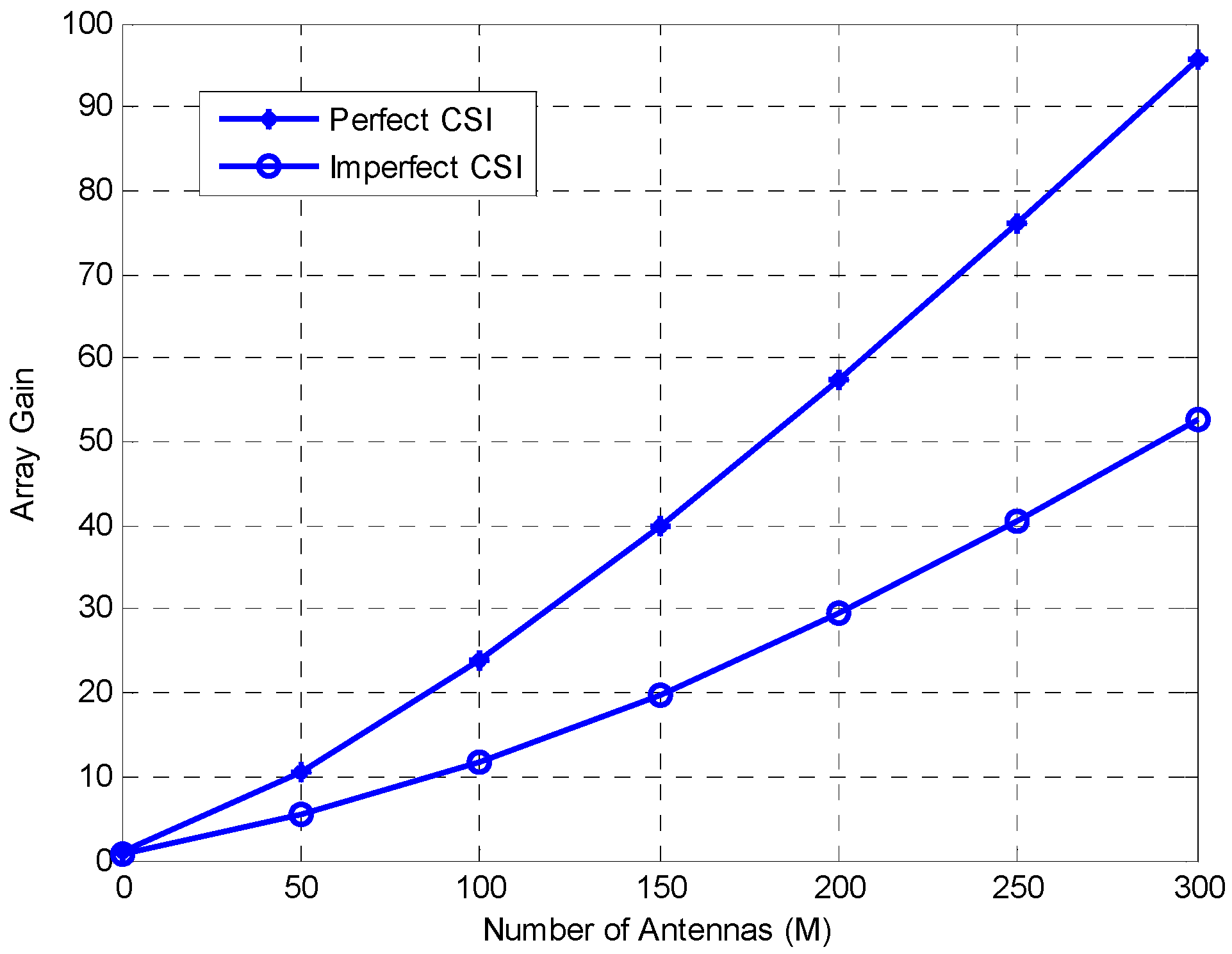
In Figure 5, array gain is plotted with different values of base station antennas (M). With massive MIMO system as the numbers of antenna increases without boundaries, the efficiency of transmit power will increase which it means the received power will also increase. High array gain is possible relying on how much the transceiver “base station” knows about the channel state. Figure 5 is plotted for the array gain under two considerations, perfect and imperfect channel state information in multi-cell system. Array gain is high with massive MIMO system as the number of antennas increases, i.e., “the transmission SNR rises with M”. The reduction in the curve is due to the fact that MRT is better at low SNR. With imperfect estimation, array gain deteriorates due to interfering of non- orthogonal pilot sequences from users in other cells which it makes pollution in channel estimation, hence the system performance is degraded.

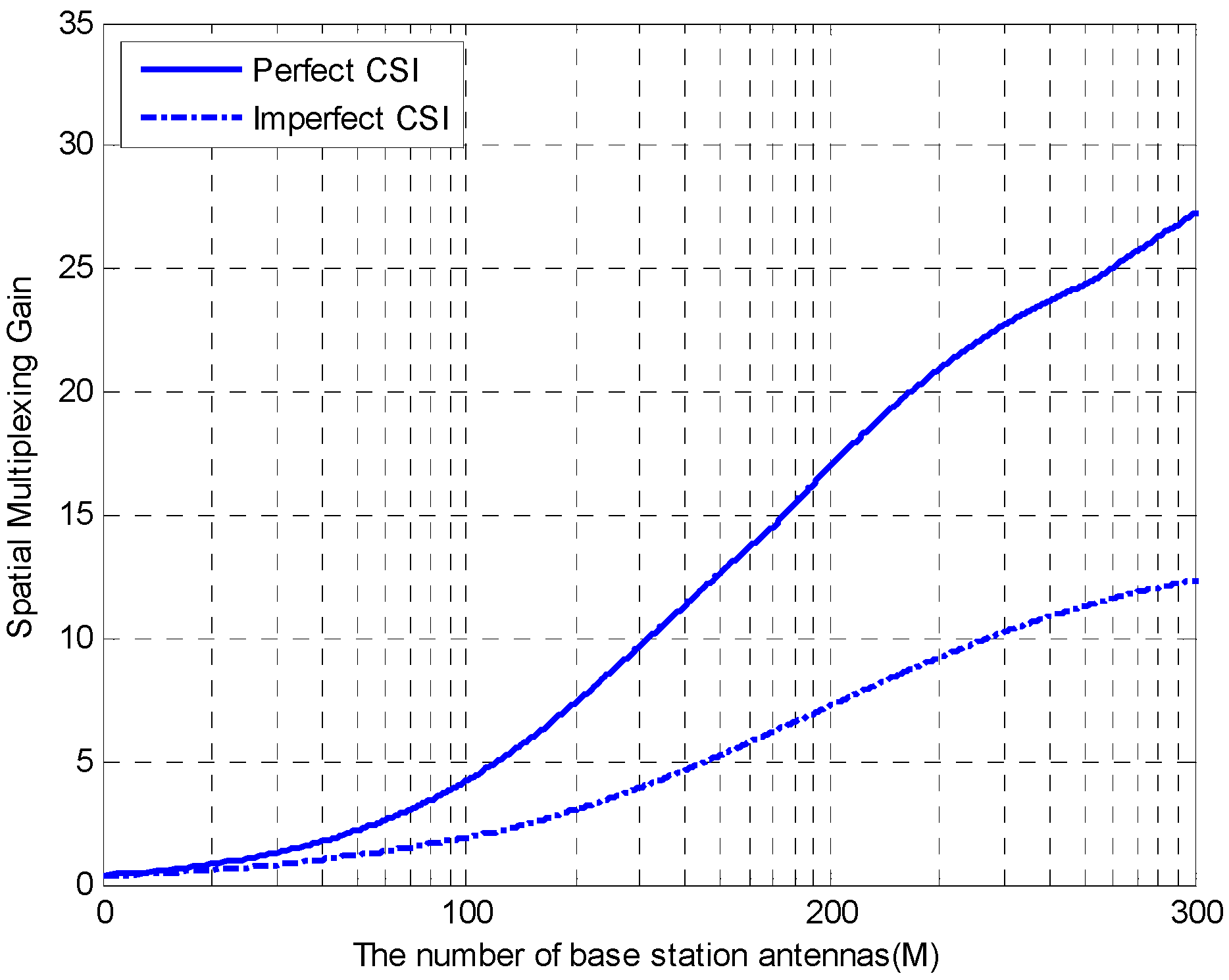
In Figure 6, the spatial multiplexing gain is drawn with the number of antennas (M) under perfect and imperfect channel estimation with multi-cell system. At favorable propagation conditions such as expressions (19) and (20) with i.i.d propagation channel matrix, the multiplexing gain rises with increasing the number of base station antennas. Consequently, the number of served terminals also increases (i.e., more degree of freedom provided). With perfect CSI, as the number of transceiver's antennas rises, the degree of freedom offered per users increases, which means more users are served through the same time and frequency, hence the system can achieve the sum rate of massive MIMO when M >> K “high multiplexing gain”. Practically, multiplexing gain impacts with the interfering pilot sequences in multi-cell system, hence low signal to noise ratio faced by two practical considerations, firstly, the terminals that are at the edge of a cell (terminals near the cell edge will suffer pollution in their received signal from neighboring cells due to reuse of non-orthogonal pilot signals in multi-cell system). Secondly, in reality the separation between antenna elements are not well (as in massive MIMO), so spatial correlation may occur which means the large number of degree of freedom will not be offered by propagation environment and this will limit the multiplexing gain under imperfect CSI. With massive MIMO, extra antennas may boost the transmission SNR and increases the multiplexing gain. For comparing massive MIMO and conventional MIMO in terms of multiplexing gain, large scale system “Massive MIMO” outperforms better than conventional MIMO due to increase the number of antennas and the number of terminals that are served simultaneously within the same coherence interval.

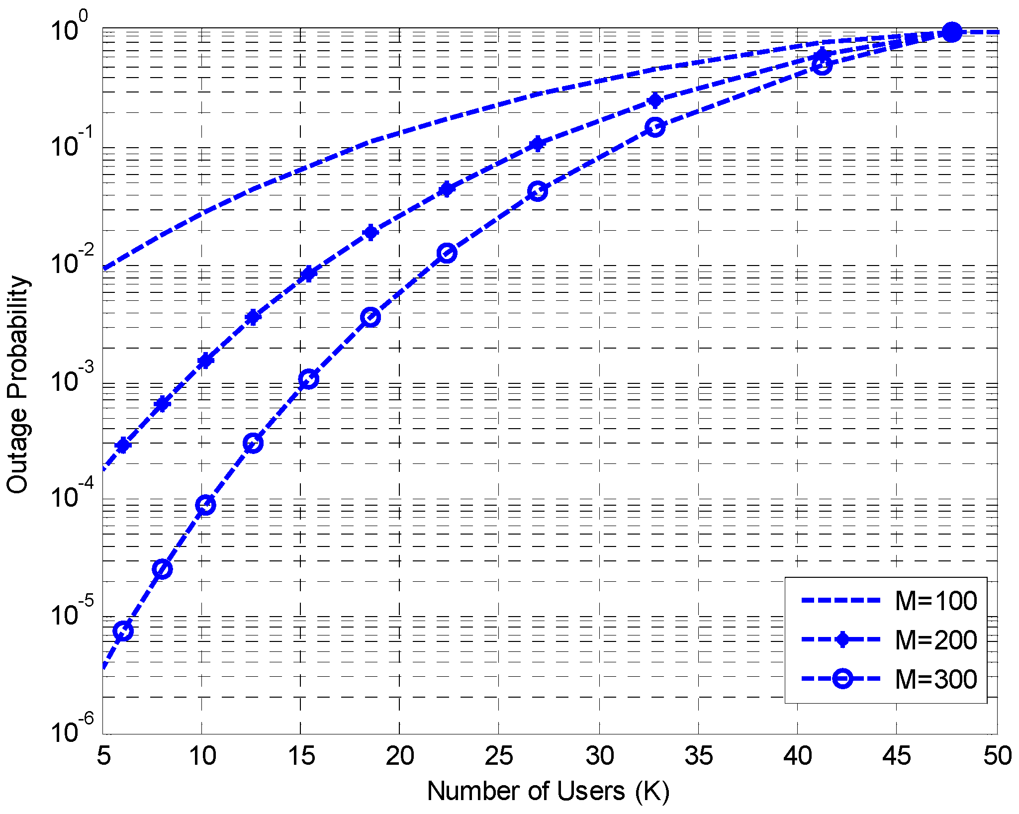
In Figure 7, as the number of antennas increases, outage probability of kth user improves also. This result can be expected for the large scale system under perfect propagation conditions, i.e., (independent, identically distributed i.i.d flat fading channels), where such system offers a large degree of freedom but practically with multi-cell massive MIMO systems, base station depends on channel state information to make estimation of channel matrix and due to non-orthogonal interfering channels among cells outage probability degraded. This deterioration rises as the number of served users K increases proportionally with rising number of antennas M in massive MIMO. Figure 7 studies also the relation between increasing the number of served terminals and outage probability occurrence with a different number of antennas (M). From the plotted figure, increasing the number of served users coherently will raise the likelihood of occurrence for outage probability, this returns to the interference among neighboring cells that use the same non-orthogonal pilot sequences. As a result with massive MIMO system, the increment in number of base station's antennas without limits can enhance the possibility of outage probability occurrence, which leads to improved spatial diversity gain.

In Figure 8, the transmitted SNR is plotted with outage probability in a multi-cell system, increasing the number of antennas will improve the outage probability through the high SNR regime. From the plotted graph, increasing the number of propagation channels will increase the number of served terminals which means the system will suffer interference from other cells due to the reuse of non-orthogonal pilot signals in a multi-cell system. In addition, Figure 8 discusses the tradeoff between the spatial diversity gain and spatial multiplexing gain if a number of users is fixed, increasing the number of antennas will improve the outage probability which means increasing the degree of freedom or enhancing the diversity gain for user. On another hand, increasing the number of propagation channels, it will increase the achievable sum rate, i.e., “spectral efficiency”, which leads to improve the multiplexing gain. However, in multi-cell large scale systems with an unlimited number of propagation channels, the number of served users differs every coherent interval will worsen the outage probability due to inter-cell interference and degrade diversity gain, while increasing the number of served terminals will increase the spectral efficiency and enhancing the multiplexing gain. However, with a multi-cell massive MIMO system under the effect of pilot contamination, the achievable sum rate will degrade due to inter-user interference among cells which leads to decrease the multiplexing gain.

In Figure 9, spectral efficiency is plotted vs. energy efficiency with various circuit power conditions under the effect of pilot contamination in multi-cell system. Energy efficiency degrades due to increase circuit power consumed for each antenna and the impact of non-orthogonal interference from other cells i.e., (interference factor β is changing from 0.01 to 0.11), spectral efficiency degrades, as the degree of interference among cells is high. In spite the effect of circuit power consumed, array gain and spatial multiplexing gain will degrade due to interference of non-coherent channels among cells. Degree of channel estimation will limit array gain loss while interference from non-perpendicular channels of other cells will limit the degree of freedom that is introduced for each user, hence decreasing the spatial multiplexing gain. Massive MIMO strengthens these gains via increasing the number of antennas.

Figure 10 explains how increasing the number of antennas will raise the achievable sum rate under perfect and imperfect CSI in massive MIMO multi cell system. As mentioned before growing the number of radio propagation channels will increase the degree of freedom which means growing the number of served terminals via coherence interval, i.e., “high spatial multiplexing gain”. The gap between the curves is due to MRT precoding, which is limited by interference due to the reuse of non-orthogonal pilot signals in a multi-cell system.

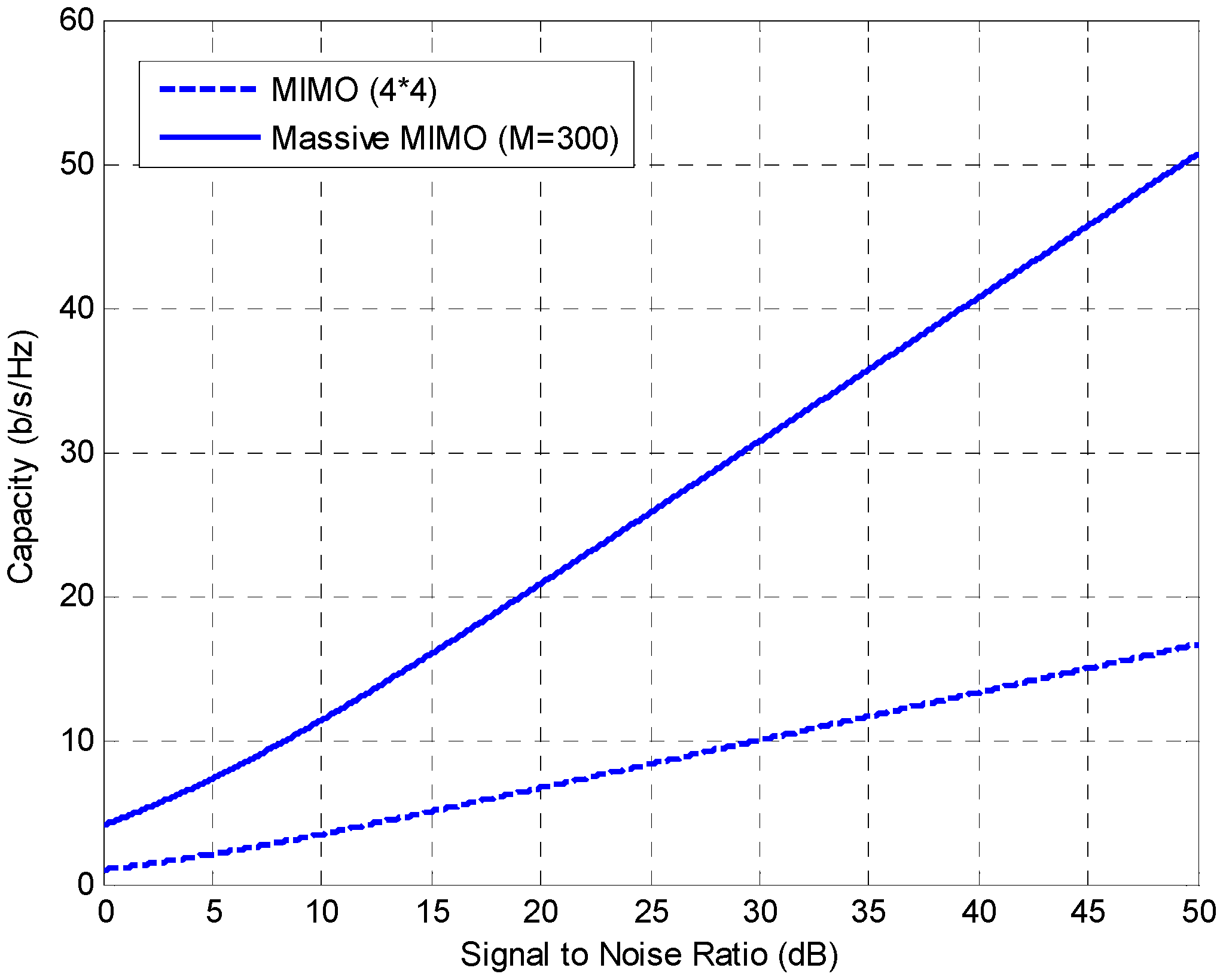
In order to compare our results for massive MIMO with conventional MIMO, Figure 11 shows this comparison in terms of channel capacity for different values of signal to noise ratio (SNR). From Figure 11, channel capacity of conventional MIMO system increases linearly as the number of antennas grows up due to the following: (1) Exploiting the spatial multiplexing concept which it is so potent technique for increasing link capacity at high SNR levels; (2) Relying on maximum number of spatial data streams which it is bounded by the minimum number of antennas at the transmitter (base station) or receiver (single user). In the other side, the link capacity of massive MIMO system outgrows the link capacity of conventional MIMO system because of the following: (1) Exploiting Space Division Multiple Access (SDMA) technique that uses spatial multiplexing concept to enable higher data rate; (2) Higher comprehensive multiplexing gain is get according to the minimum number of antennas at users (multi-users are served simultaneously which induces for higher data rate) as mentioned before in Theorem 2.

Figure 12 shows that the massive MIMO technique outperforms conventional MIMO technique by enhancing system performance in term of outage probability through beamforming technique, which it is defined as a downlink multi-antenna technique weights the data before transmission, forming narrow beams and aiming the energy at the target user, then it improves the spatial diversity gain in massive MIMO via increasing the received SINR. As compared to conventional MIMO technique, massive MIMO technique will give the following important features of increasing the number of antennas in mobile communication systems: (1) Hiding the effects of thermal noise, fast fading and intra cell interference among users; (2) Rising the degree of freedom that were provided for serving terminals which means more robustness and link reliability (i.e., increased diversity gain); (3) Reducing uplink and downlink transmit powers through coherent combining and increasing antenna aperture, transmit power of each user terminal can be reduced inversely proportional to the number of antennas at the BS with no reduction in performance.

6. Conclusions

The main performance gains in a multi-cell massive MIMO system (array gain, multiplexing gain and spatial diversity gain) are discussed for first time at this work taking into account the effect of pilot contamination on massive MIMO system through these gains. These gains mirror the energy efficiency, spectral efficiency and channel reliability with its effect on the performance of massive MIMO systems. Fundamental tradeoffs among these gains are studied and the present work concludes that all gains cannot be maximized at the same time due to non-orthogonal interference among cells. Our simulation results discussed the effect of pilot interference on the tradeoff between energy efficiency and spectral efficiency. In addition, a comparison is made between imperfect and perfect CSI on array gain and multiplexing gain. Still massive MIMO outperforms because of unlimited number of antennas that makes it powerful to any interference.