1. Introduction
The principle of absorption cooling was first described by the French scientist Ferdinand Carré in 1858. The original design used water and sulfuric acid, and in 1926 Albert Einstein proposed an alternative design, the Einstein refrigerator. Commercial production of absorption refrigeration units began in 1923 by AB Arctic, which was bought by Electrolux in 1925 [
1]. Small capacity powered diffusion absorption refrigerators have been commercially produced by Electrolux since 1928 [
2]. Designed as domestic refrigerators for small portable applications and for hotel rooms, they had cooling capacities of a few tens of watts and COP's generally fell between 0.1 and 0.3. The performance of the devices has been assessed during the last half century by various researchers such as Watts and Gulland [
3], Stierlin
et al. [
4], Backstrom and Emblik [
5] and Chen
et al. [
6]. Jacob and Eicker demonstrated that large scale absorption coolers and chillers in excess of 20 kW could be economically viable if powered by waste heat from industrial processes [
7]. This endeared two lines of research: small scale CHP/tri-generation and solar power absorption cooling. In the beginning of the 21st century, the University of Stuttgart obtained grants from the Joule Craft program to develop a single stage ammonia-water diffusion absorption cooling machine with a capacity of 2.5 kW [
8,
9,
10]. The first two machines failed to reach their design capacity and lost performance in operation. The third prototype developed and subsequently modified in 2006 eventually gave a cooling capacity of 2.0–2.4 kW at 18–15 °C respectively with an average COP of 0.3 corresponding to a source of 125 °C.
Around the same time, Bales and Nordlander investigated the characteristics of the thermo chemical accumulator (TCA) of a commercially available unit [
11]. The TCA is a three-phase absorption heat pump that stores energy in the form of crystallized salt (Li/Cl) with water being the other substance. They estimated the thermal COP to be 0.7 but could not verify this in the laboratory testing. Bales
et al. showed that the thermal storage of a TCA is sufficient for small scale solar cooling applications that do not have large night cooling loads [
12]. Sanjuan
et al. investigated the advantages of salt desiccants, like Lithium-Chloride (LiCl)
versus liquid absorption systems [
13]. Their major finding is that the absorption process and the energy storage is combined in one so that the production of cooling energy can be decoupled from the solar gains without external storage tank. They show that these units are able to substitute big absorption systems due to the small size. They also show good adaptability and many possibilities of operation for medium and small scale systems. The Lithium-Chloride-water pair has been tested by ClimateWell and is currently used in their solar absorption cooling technology [
14]. They have shown that this pair is not suitable for seasonal storage due to its high cost of the salt. However the system can deliver either cooling or heating and the problem of crystallization has been overcome and that enables the enhancement of the storage density and COP with a so-called “closed three phase absorption”. They indicate a cooling COP of 0.68; however installed systems usually manage a COP in the range of 0.52–0.57.
This paper presents in a first instance, a computer model for the prediction of the COP of a thermo-chemical accumulator unit based on the design parameters. The input data consists of temperatures for the heating load, heat sink and cooling circuit as well as their respective flow rates. In a second instance the model is used to estimate the COP of a TCA unit when run on hot water from biomass combustion as the heat source. Although the system is developed to run on solar heating (heat source temperatures around 110 °C) compared to the lower heart source temperature available from domestic hot water boilers run on biomass, the authors expect feasible operating conditions.
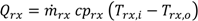
2. Thermodynamic Analysis of LiCl Absorption Cooling
The thermo-chemical accumulator (TCA) is an absorption process that uses a working pair in the liquid, vapor and solution phases as well as a solid sorbent. This process is significantly different from the traditional absorption processes in that it is a three phase process (solid, solution and vapor). All other absorption processes are two phase processes with either solution + vapor or solid + vapor. A typical thermo-chemical accumulator unit consists of a reactor and condenser/evaporator with a vapor channel between them, as well as tanks for both water and the active salt solution. Vacuum conditions are assumed and each of the main sections has its own mass and associated heat loss coefficient. Heat of vaporization, condensation and dilution are taken into account and a single UA-value (overall heat transfer coefficient for the whole heat exchanger area) is used as a parameter for charge and discharge conditions. These UA-values are used to calculate the UA-values for the reactor and the condenser. The parameters for the LiCl solution and crystals were obtained from the manufacturer and/or taken from reference textbooks [
15].
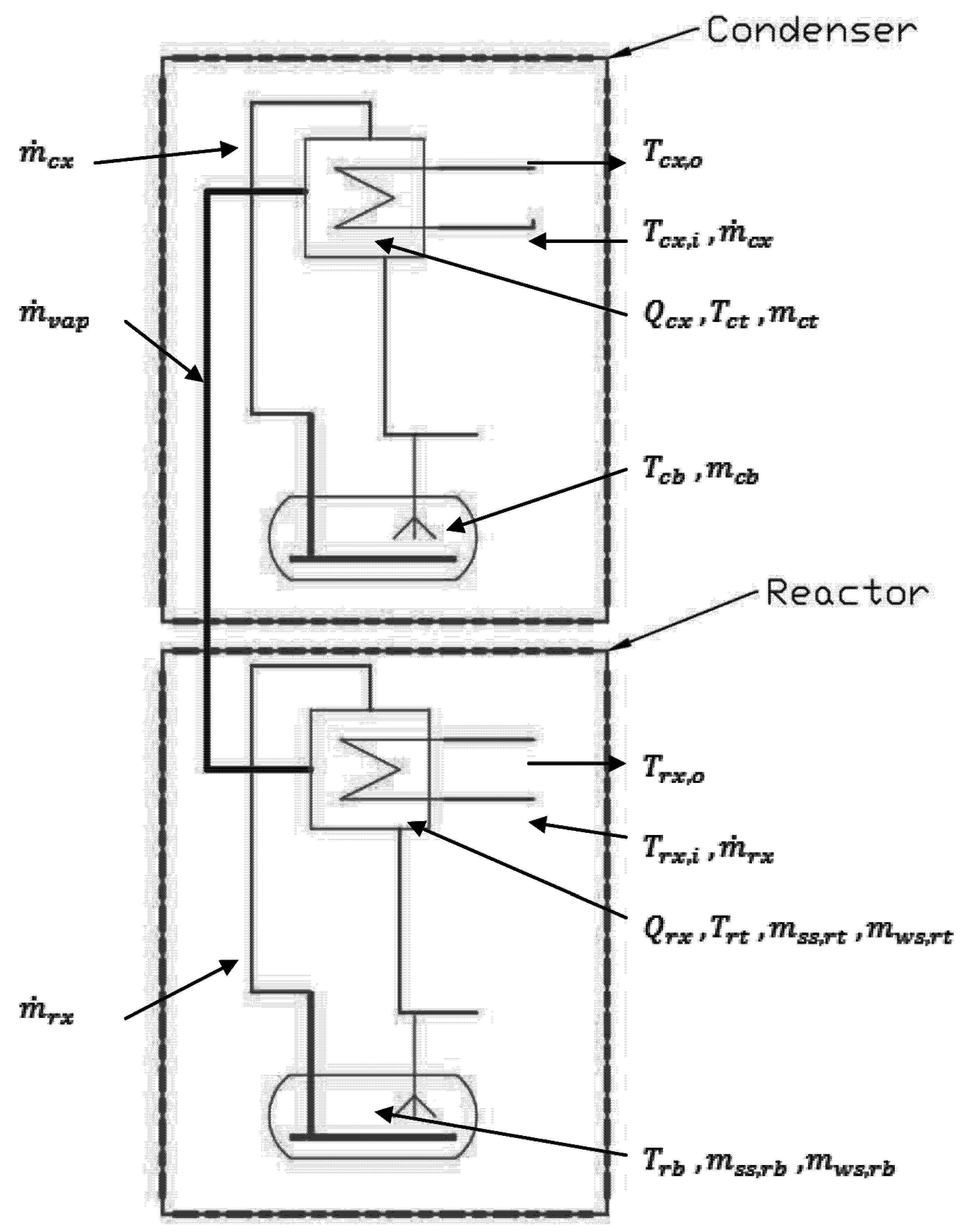
Figure 1.
Schematic drawing of the thermo-chemical accumulator (TCA) unit.
Figure 1.
Schematic drawing of the thermo-chemical accumulator (TCA) unit.
For simplicity, the condenser and the reactor are treated as though they each consist of two separate tanks. A schematic representation of these tanks can be seen in
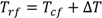
Figure 1. This allows considering the top tank as the exchange of energy between the tank and the outside, and the bottom tank as a store for the water or salt solution. Internal pumps assure the exchange of water/solution between the bottom tank and the top tank. Thus the condenser top is the condenser itself and the condenser bottom is the water store. Likewise, the reactor top is the reactor itself and the reactor bottom is the solution store. It is assumed that in initial conditions, all salt is dissolved in the reactor. In the real system, the temperatures depend on the heat transfer across the heat exchangers. Similarly, the masses and the salt concentrations are dependent on the temperatures. In order to express this mathematically, it is assumed that the system determines its initial conditions then evaluates its corresponding temperature and mass values. They are constantly being adjusted to adhere to the principles of mass and energy balance. Thus, symbols on the left hand side of the subsequent equations refer to the adjusted values whereas the ones on the right hand side refer to the outdated values. Initially all the temperatures for the reactor and condenser are set to the ambient temperature. The concentration of the solution can then be calculated as follows, depending on the quantities of water and salt in the respective tanks:
Based on this calculated solution concentration, the mass of water and solution in every part of the unit can be calculated, based on the volume of the reactor and the density of the salt, as follows:
mass of salt solution in the reactor top
mass of water solution in the reactor bottom
mass of salt solution in the reactor bottom
mass of water solution in the reactor bottom
Applying the principles of mass and energy transfer to any heat exchanger can be expressed mathematically as (adopted from Kays and London [
16]):
Here cp is adjusted based on mean temperature between out and return flow of the corresponding circuit (i.e., heat source, heat sink or cooling). The absolute value for the temperature difference is used to avoid a negative value for Q in the subsequent equations for evaluating the COP.
Thus, for the condenser heat exchanger power,
for the reactor heat exchanger power,
for the energy rate due to vapor for the condenser,
and for the energy rate due to vapor for the reactor,
The mass fraction of LiCl salt in the reactor is given as follows:
The temperature difference between the reactor and the condenser during equilibrium is based on this salt concentration. Equilibrium is assumed when both mass and energy balances are satisfied. Equation (13) gives the expression of this temperature for Lithium Chloride, which is fitted to data extrapolated from Conde [
17].
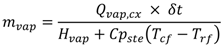
The energy rate due to vapor in the condenser depends on the UA value of the heat exchanger in the condenser, the temperature of the water film on the heat exchanger surface as well as the temperature of the condenser top. The film temperature of the condenser can be determined from the above heat transfer equations as follows:
The energy rate due to vapor in the reactor can be calculated via the vaporization and differential enthalpy of dilution. When the system is charging, part of the heat is used to vaporize the water and the rest to break the bond to the salt. If the system is discharging, then the energy stored by the salt is released because of the dilution of the salt solution and the condensation of the water vapor. The film temperature at the reactor heat exchanger can be determined as follows:
The mass of vapor is dependent on the energy rate due to vapor and the film temperatures of the surfaces of the heat exchangers.
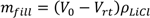
The mass migrations between the reactor and the condenser due to vapor transport could go in either direction depending on whether the unit is charging or discharging. During the charging process, the vapor travels from the reactor to the condenser and vice versa for discharging. Therefore (for charging), some part of the water in the top tank of the reactor will go to the condenser and some solution will be pumped up to the top tank from the bottom one, so that the mass of solution in the top tank will be kept constant. This can be expressed mathematically as follows:
From Equations (18) and (19) the volume of the reactor top tank and the required mass to fill it up can be evaluated as follows:
There are three possibilities for Equation (19): the bottom tank is empty (mfill = 0), the solution is pumped from the bottom tank to the top (mfill > 0), or the solution is pumped from the top tank to the bottom (mfill < 0). Depending on what direction the solution is being pumped, the masses of LiCl salt and water in the reactor can be determined according to the mass conservation equation and for adjusted values for the masses of solution and water.
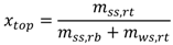
The LiCl concentration and temperature of the top and the bottom tank can be determined using the mass and energy conservation principles as follows, based on the masses in the reactor:
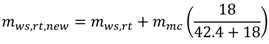
The required amount of monohydrate crystals can be evaluated depending on Conde's published data for the concentration of crystals and based on the molecular masses for Lithium-chloride (42.4 g·mol−1) and water (18 g·mol−1):
The transport of the vapor can cause the solution in the top of the reactor to be concentrated or diluted. Therefore, extra water or salt is required to keep the salt solution at its equilibrium state. The temperature changes, due to the dissolution at the reactor top, can be expressed as follows:
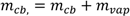
If there is not enough solution of water available, then the required mass of monohydrate crystals is set to zero and the masses of the salt and water solution are adjusted:
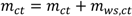
The calculations for the condenser are less extensive as they are largely dependent on the calculations carried out for the reactor. The mass of the condenser bottom tank is dependent on the flow of vapor:
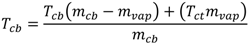
The temperatures of the condenser top and bottom tank are dependent on whether the unit is charging or discharging. For charging (mvap > 0):
For discharging (mvap < 0):
Additionally the condenser temperatures need to be adjusted to account for the internal mixing of the pumps as follows:
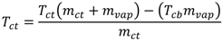
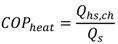
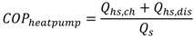
The coefficient of performance (COP) is the ratio of output to input energies. COP
cool is the thermal COP for producing cooling from the thermal source, and COP
heat is for the heat extracted during discharge for the given operating conditions. COP
pump is the thermal COP if the machine is used as a heat pump, with the energy that in cooling operation is dumped to ambient, being used for heating. The heat input (
Qs) as well as the heat outputs (
Qac,
Qhs) is determined trough Equation (6). The actual values are based on whether the system is charging or discharging as indicated in
Table 1.
Table 1.
System connections to the surroundings depending on status.
Table 1.
System connections to the surroundings depending on status.
| Status | Heat source (Qs) | Heat sink (Qhs) | Cooling (Qac) |
|---|
| Charging | Reactor | Condenser | |
| Discharging | | Reactor | Condenser |
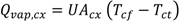
3. The Computer Model
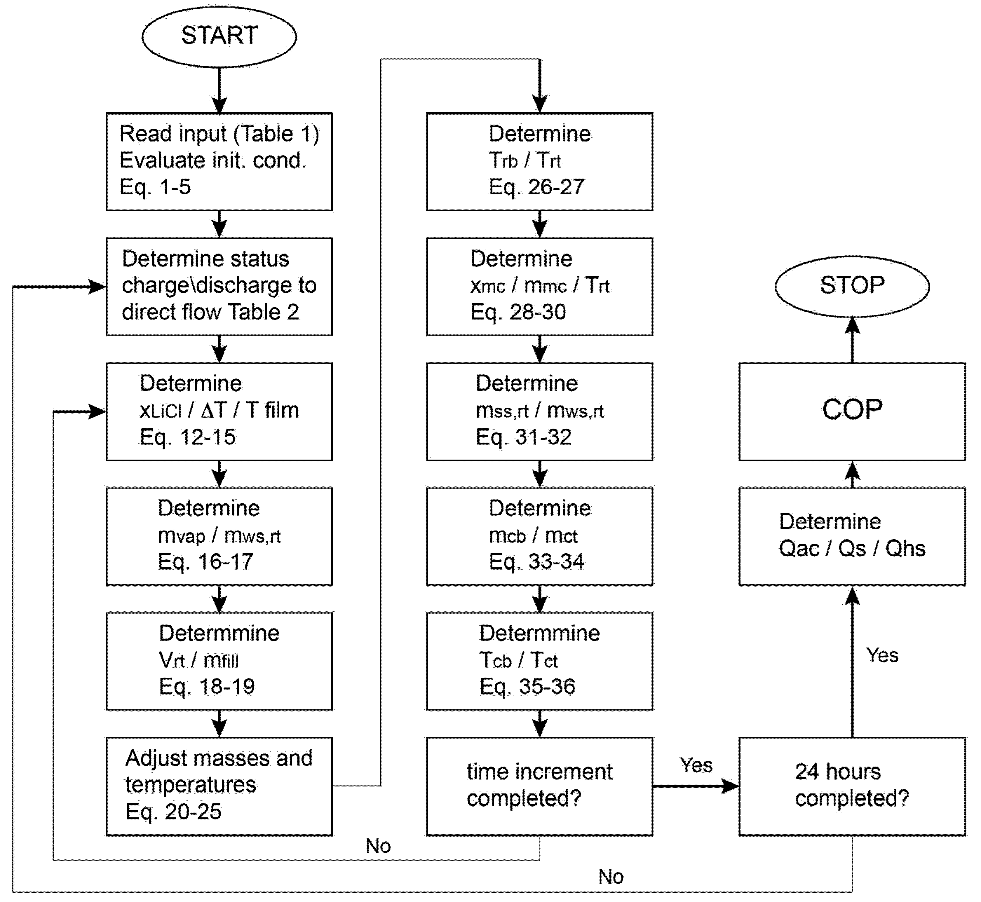
The TCA system used in this project is comprised of two barrels and a control unit. The control unit regulates the pumps in the system and determines which barrel is being charged and discharged. There are no calculations involved and the whole process is based on decision (If...else) statements depending on the information supplied to the control unit from the temperature sensors built into the system. The model uses a fixed number of internal time steps for every output time step in order to iterate to a solution. The condenser and the reactor are treated as though they each consist of two separated vessels. The top vessel is used to exchange energy between vessel and outside, and the bottom vessel is used to store the water or salt solution. The control unit is used to regulate the internal pumps as well as the overall charge level of the reactor. Similar to the actual machine, the barrel is charged to a certain limit, before a swapping procedure is initiated. This swap period allows the systems to redirect flow and regulate the speed for the internal pumps. Since the system will always charge one unit while the other one discharges, the heat source and the distribution system are only ever connected to one internal circuit whereas the heat sink is always connected to two circuits. To account for this, the flow rate for the heat sink is divided by two in the model. The system constantly monitors the level of charge/discharge of the unit. A unit is considered fully charged when the salt concentration in the reactor reaches 95% and cannot be “dried” any further. Similarly, a unit is considered being fully discharged when the water level in the water store goes below 12 kg. In this model a swap will occur only when a unit is fully discharged.
For simplicity, the inlet temperatures to the system are kept constant for all three circuits. Obviously, in reality this is not the case and they fluctuate depending on the use of the circuits. For example, the heat sink return temperature largely depends on the capacity of the circuit to dissipate the heat from the incoming water and its temperature. The time length of the simulation is set to 24 h. This timeframe is used to assure at least one complete instance of charge and discharge of the barrel is carried out with at least one instance of swapping. The model iterates for a set number of times between each time increment. The following steps (
Figure 2) are carried out in each iteration of the model.
The temperature difference between the reactor and condenser based on LiCL concentrations
The energy transferred by the water vapor
The vapor flow rate and heat exchanger outlet temperatures
Mass of solid monohydrates LiCl crystals and resulting temperature changes
Temperatures and mass changes due to mass transfer of water vapor
Temperatures and mass changes due to internal solution flow
Figure 2.
Program flowchart of the coefficient of performance (COP) evaluation model.
Figure 2.
Program flowchart of the coefficient of performance (COP) evaluation model.
At the beginning of each simulation, the model loads the design parameters and reads the user input. Then, Equations (1)–(5) are run to determine the initial conditions of the system. Subsequently, the model runs a number of iterative steps to reach the first time increment. At the end of each time increment, the values are updated and the model verifies the charge/discharge status of the unit and if necessary if the swap period is over. At the end of a swap, the model determines a charge or discharge status based on the previous status of the unit.
4. Results
The first run was based on the data presented in
Table 2 (optimal design values for a solar thermal heat source) in order to compare the model output with published data.
Table 3 shows the COP’s for this unit determined by the model, as well as the COPs determined by the manufacturers design calculations. Although, the cooling COP is stated as 0.68, installed systems all show a COP varying between 0.52 and 0.57. The present study estimates a COP closer to the realistic system as the published data.
Table 2.
Input data for the analytical model of the TCA unit.
Table 3.
Comparison of COP results.
Table 3.
Comparison of COP results.
| Parameter | Published data [11] | Present study | Relative error % |
|---|
| COPcool | 0.68 | 0.61 | 10.29 |
| COPheat | 0.79 | 0.69 | 14.78 |
| COPpump | 1.41 | 1.42 | −0.71 |
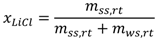
When combining
Table 2 with the information from
Table 1, it can be seen that during a charging instance, the inlet temperature for the reactor is equal the temperature of the heat source (115 °C) and the inlet temperature for the condenser is equal to the temperature of the heat sink (25 °C).
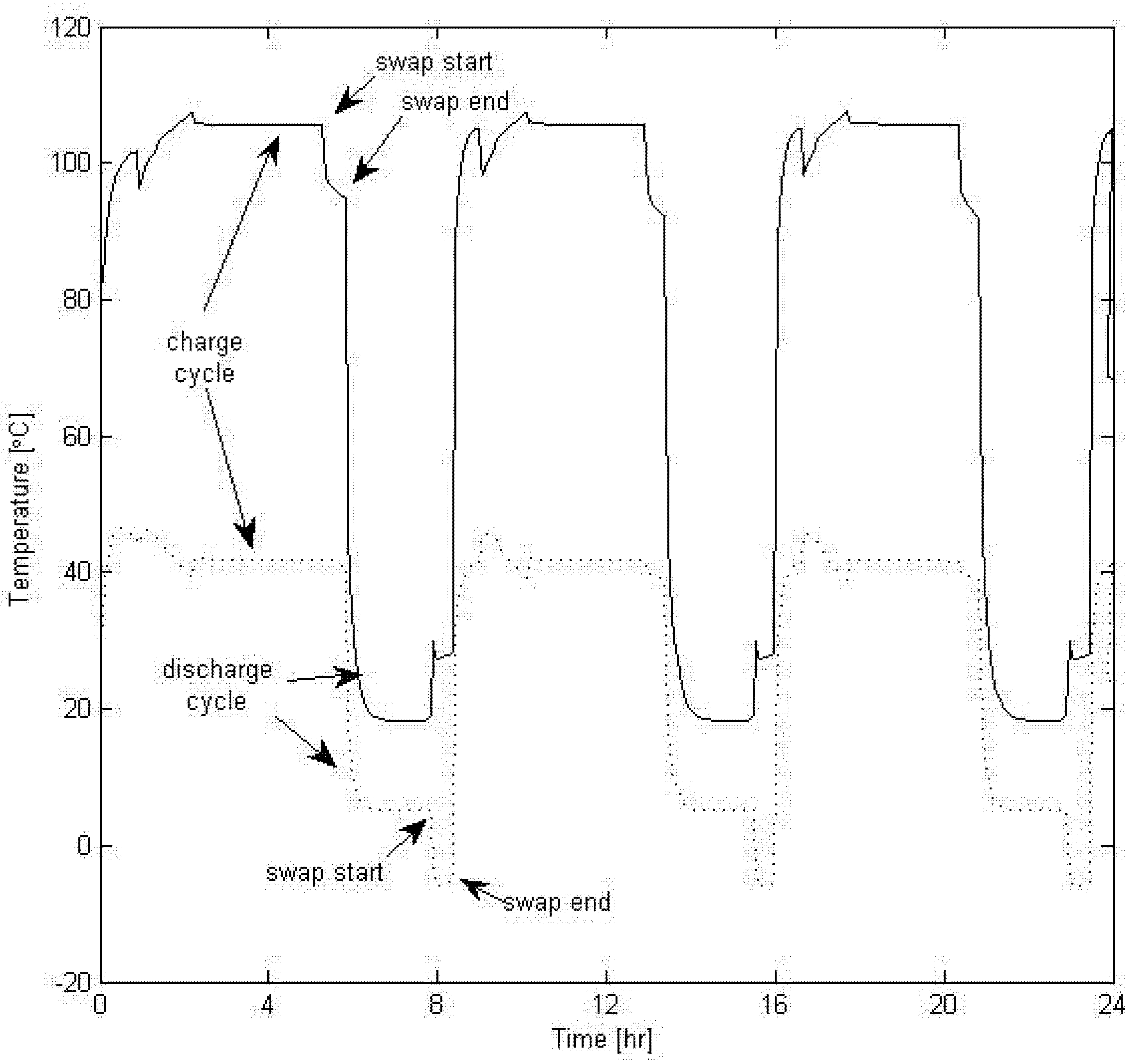
Figure 3 shows the outlet temperatures for the condenser and reactor. The drop in temperature in the discharge phase is corresponding to providing cooling. However, the temperatures will differ in the real system as inlet temperatures are not constant but vary according to their load.
Figure 3.
Outlet temperatures for condenser and reactor.
Figure 3.
Outlet temperatures for condenser and reactor.
It is assumed that all mass flow rates and specific heat capacities are kept constant, and thus the heat is only dependent on the temperature changes. From Equation (39), it can be deduced that an increased COP is due to either an increased cooling output with constant heat input or that the rate of heat input is smaller than the rate of cooling output. Similar it can be said that a decrease in heat input will result in an increase in cooling output if the COP is increasing; and a decrease in cooling output if the COP is decreasing.
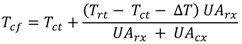
Figure 4,
Figure 5,
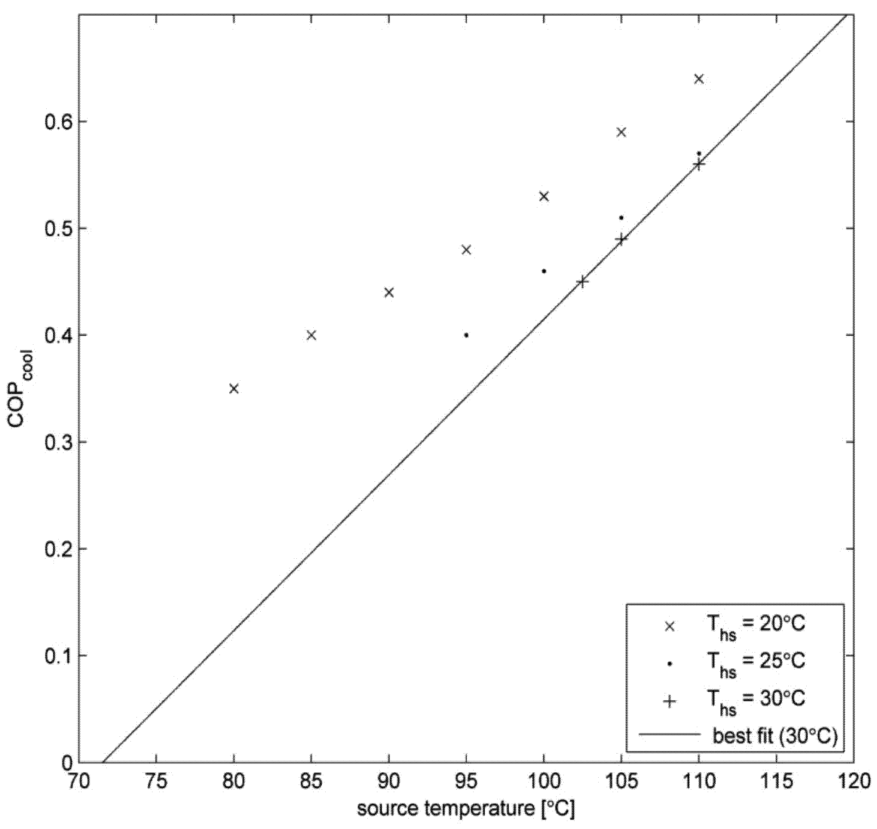
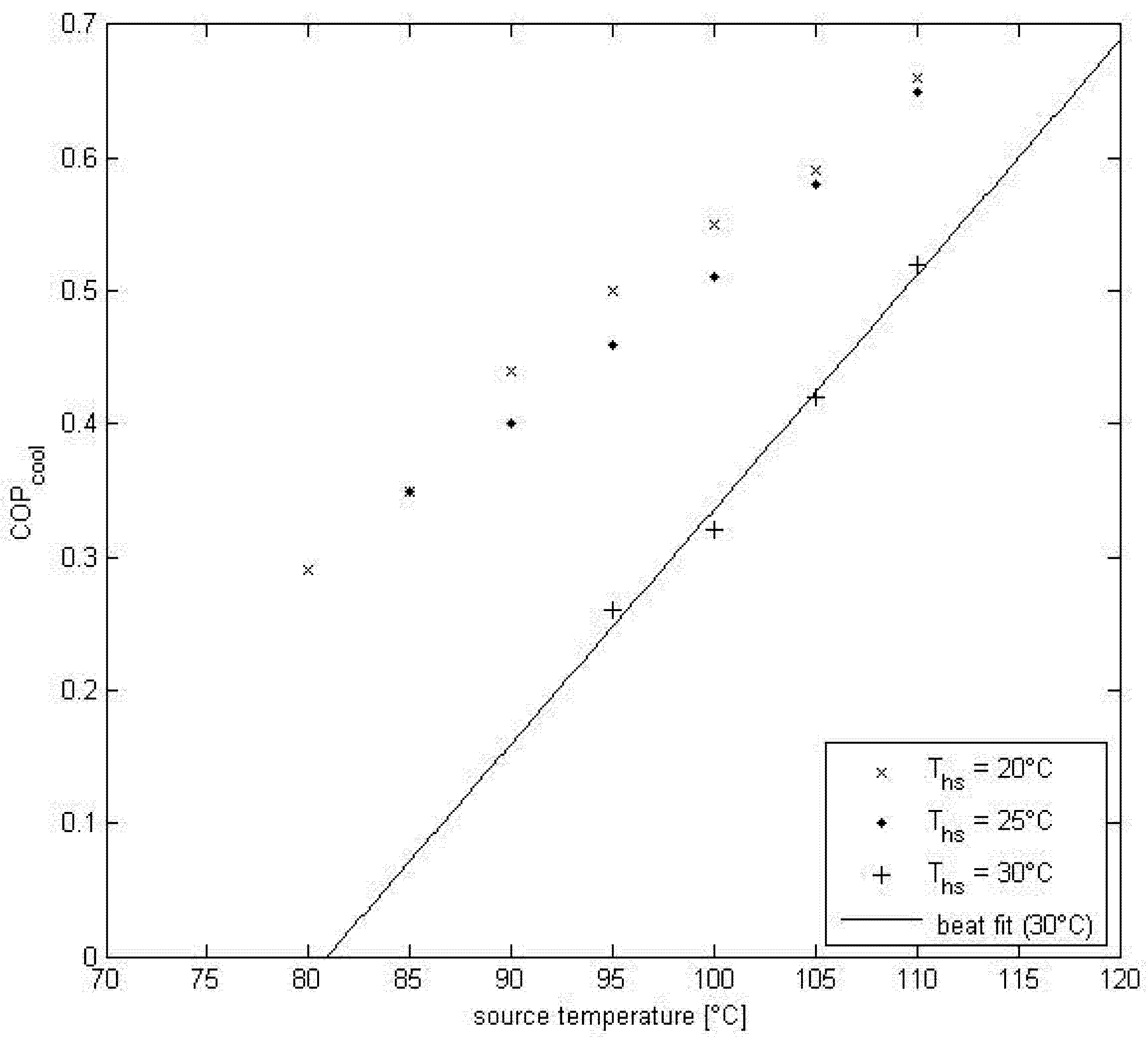
Figure 6 show a comparison of cooling COP against heat source temperature for various cooling temperature based on different heat sink temperatures. It can be seen that an increase in heat source temperature results in a higher COP while keeping the cooling temperature constant. The simulations are all run for heat load temperatures varying between 80 °C and 110 °C. For the lower cooling temperatures (18 °C and 22 °C) a high heat sink will not compute results for heat source temperatures below 95 °C. An additional data point for 102.5 °C was added for the 30 °C heat sink results. It has to be said that any other values are all outside the minimum working conditions of the unit and thus would not contribute to any useful discussion. As expected, it can be observed that the COP is improved by reducing the heat sink inlet temperature. The performance of any installed heat sink circuit is not considered in the present work.
Figure 4.
COP against heat source temperature for 18 °C cooling temperature.
Figure 4.
COP against heat source temperature for 18 °C cooling temperature.
Figure 5.
COP against heat source temperature for 22 °C cooling temperature.
Figure 5.
COP against heat source temperature for 22 °C cooling temperature.
Figure 6.
COP against heat source temperature for 26°C cooling temperature.
Figure 6.
COP against heat source temperature for 26°C cooling temperature.
Figure 4, cooling temperature set to 18 °C, shows that lowering the heat sink inlet temperature from 30 °C to 20 °C can improve COP from 0.35 to 0.65. An important aspect for this study is that lowering the heat source from 95 °C to 85 °C, the same COP can be achieved whilst applying this heat sink temperature drop. In the practical range for biomass hot water applications this gives a COP between 0.35 and 0.43.
Figure 5, cooling temperature set to 22 °C, shows that increasing the cooling temperature from 18 °C to 22 °C, decreases the COP between 0.2 and 0.5, as expected by Equation (39). However it can be observed that lowering the heat source can be compensated for by lowering the heat sink temperature as well. For heat source temperatures from 80 °C to 90 °C the COP varies between 0.3 and 0.43.
Figure 5, cooling temperature set to 22 °C, shows similar behaviour as the previous figure. The COP for the targeted heat source range varies between 0.3 and 0.44.
Figure 6, cooling temperature set to 26 °C, shows almost identical COP values as for a cooling temperature of 24 °C. This means that the rate of change for the cooling output is similar to the rate of change in heating input. Thus, there is no gained improvement by increasing the cooling temperature, nor decrease in improvement by an elevated cooling temperature depending on the climate region the system is installed in.
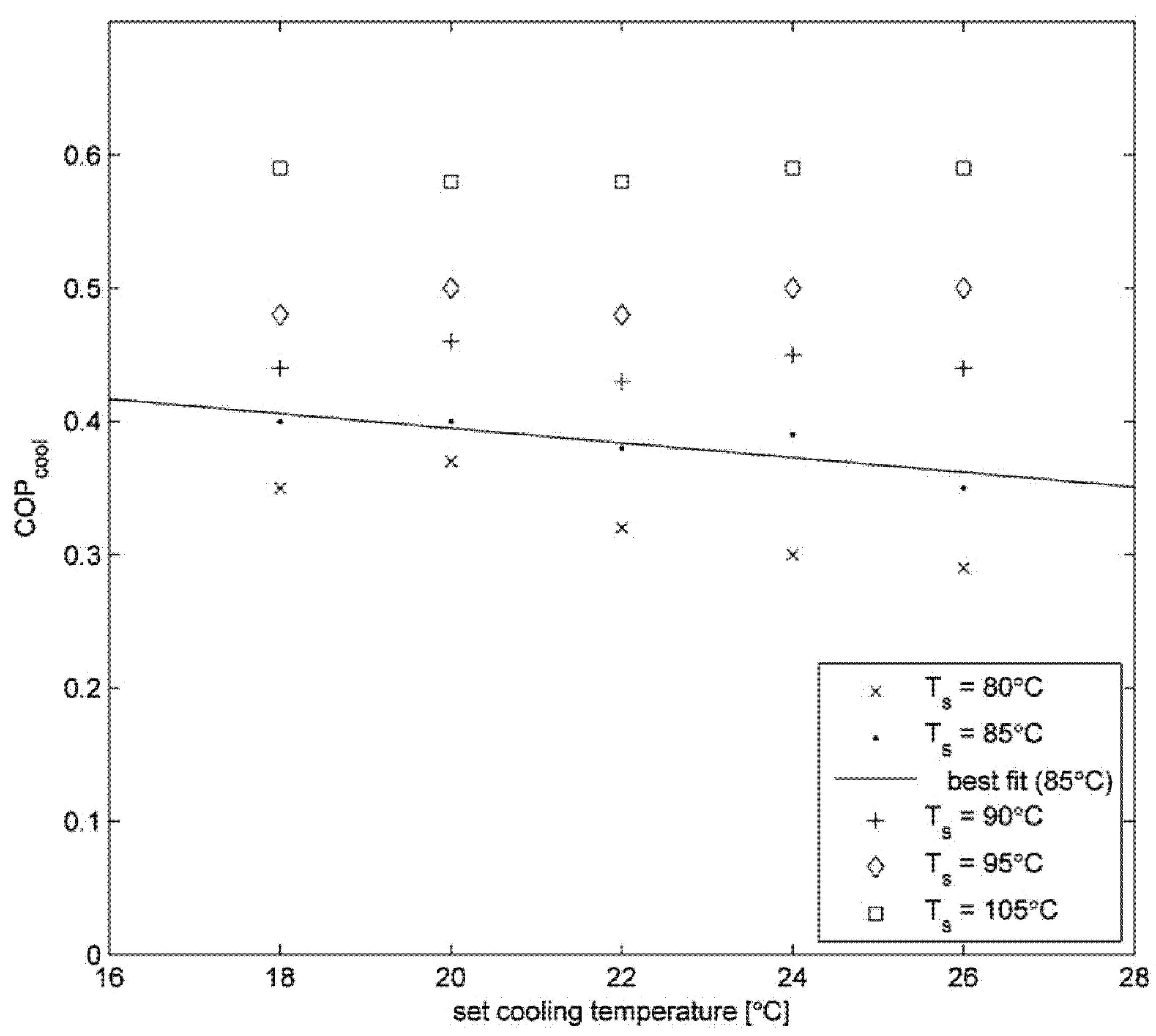
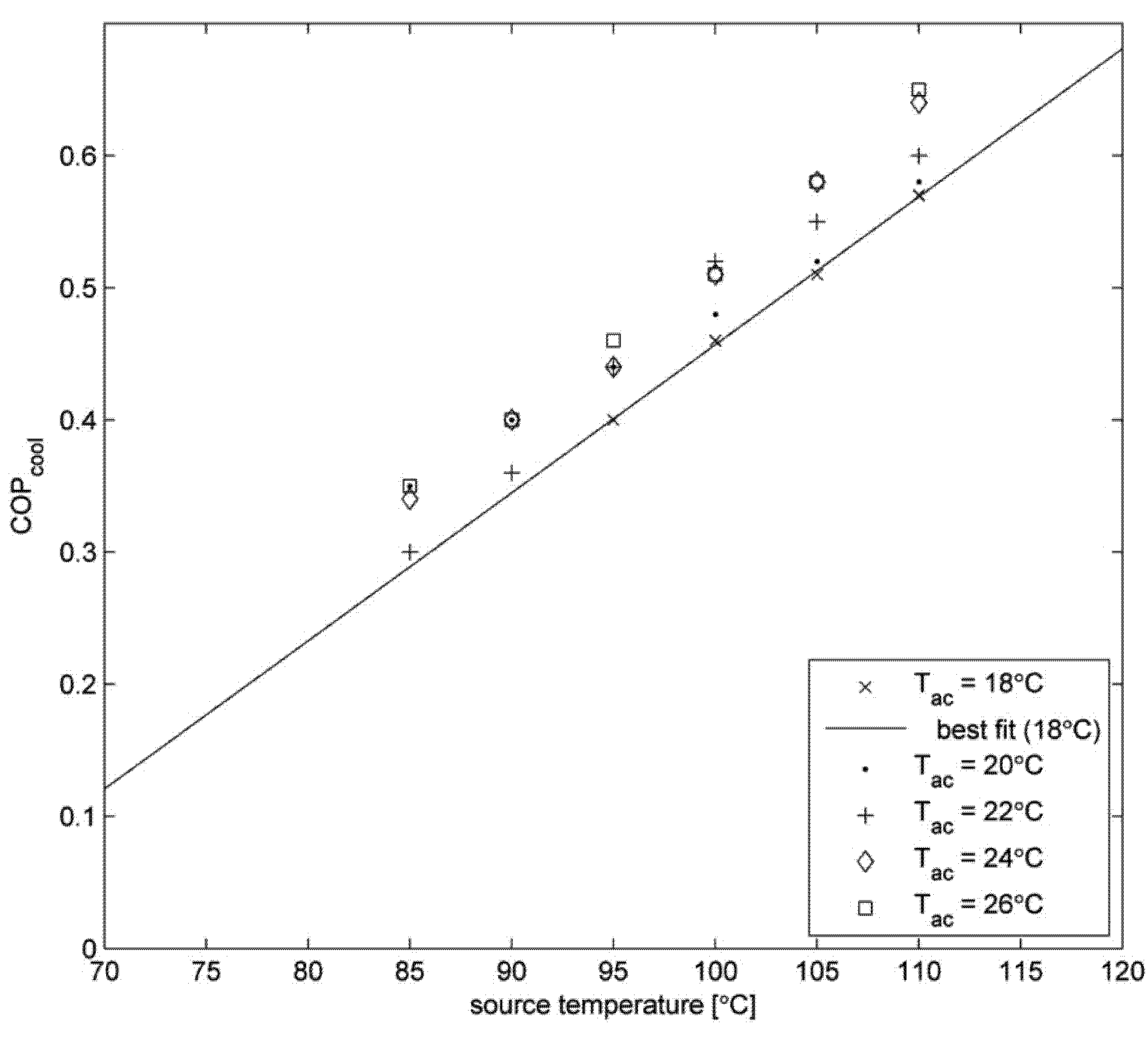
Figure 7 shows the variation of cooling COP against cooling temperature for different heat source temperature while keeping the heat sink constant at 20 °C. It can be seen that for the lower region of heat source temperature there is a decrease in COP when increasing the cooling temperature above 22 °C. In the targeted heat source range (80 °C to 90 °C) the best COP should be achieved at cooling temperatures in the range of 18 °C to 20 °C. The manufacturers actually recommend that the inlet cooling temperature should not exceed 21 °C for reasons of performance.
Figure 7.
COP against cooling temperature for 20 °C heat sink temperature.
Figure 7.
COP against cooling temperature for 20 °C heat sink temperature.
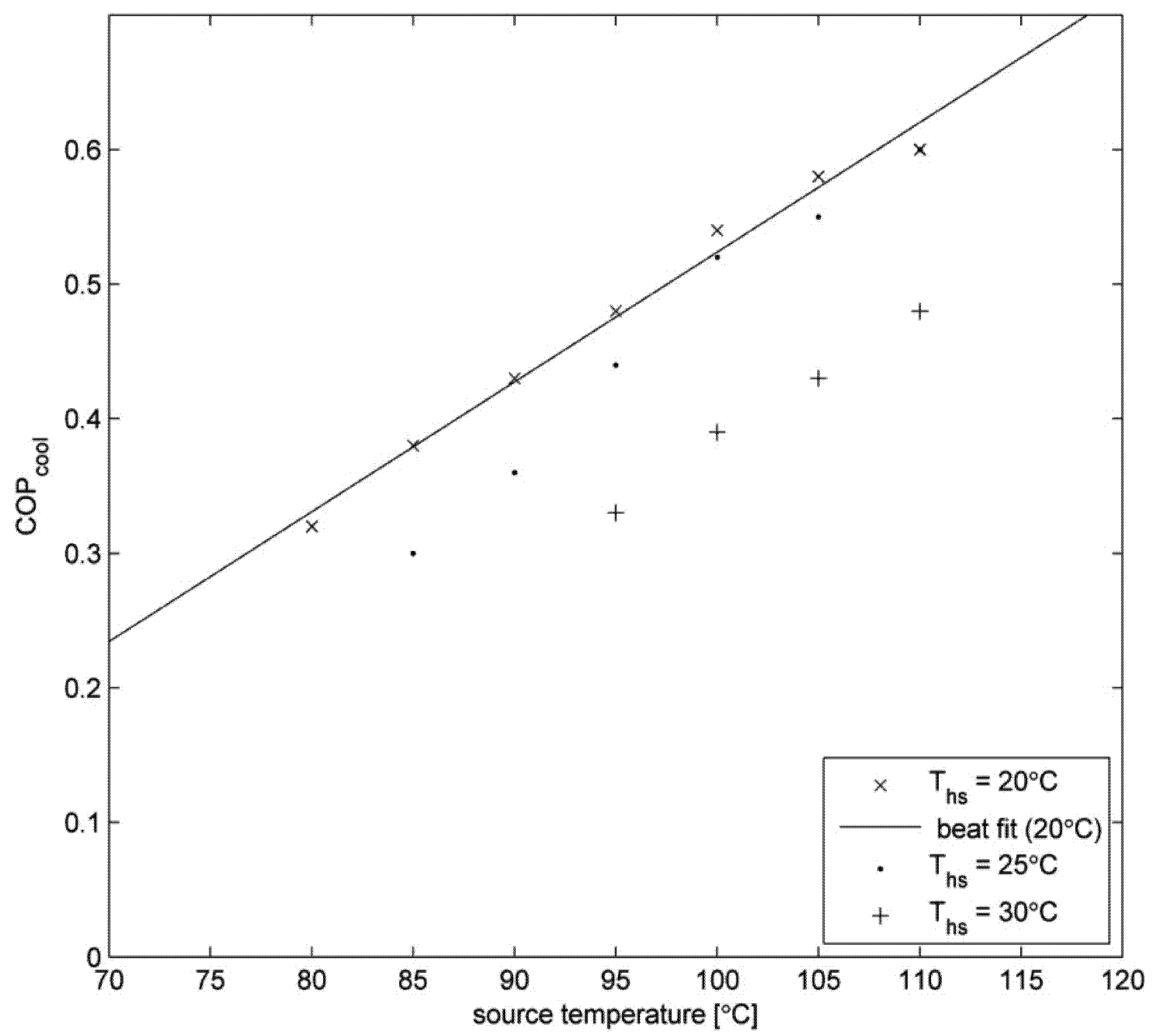
Figure 8 and
Figure 9 show the variation of COP against heat source temperature for a range of cooling load temperatures and for heat sink temperatures of 25 °C and 30 °C, respectively. As mentioned before, a lower heat sink temperature gives better results for COP and in return a higher heat source temperature will result in a higher COP. Again, this shows that the target range of heat source temperatures can be used however there will be a slight drop of the COP.
Figure 8.
COP against heat source for 25 °C heat sink temperature.
Figure 8.
COP against heat source for 25 °C heat sink temperature.
Figure 9.
COP against heat source for 30 °C heat sink temperature.
Figure 9.
COP against heat source for 30 °C heat sink temperature.


