

Improvement of the Dynamic and Seismic Behaviour of Rigid Block-like Structures by a Hysteretic Mass Damper Coupled with an Inerter

1
Department of Civil, Construction-Architectural and Environmental Engineering, University of L’Aquila, 67100 L’Aquila, Italy
2
College of Engineering, Fuzhou University, Fuzhou 350025, China
*
Author to whom correspondence should be addressed.
Appl. Sci. 2022, 12(22), 11527; https://doi.org/10.3390/app122211527
Submission received: 8 October 2022
/
Revised: 4 November 2022
/
Accepted: 10 November 2022
/
Published: 13 November 2022
(This article belongs to the Special Issue Recent Perspectives on Smart Structures and Infrastructures for Enhanced Vibration Mitigation and Health Monitoring)
Abstract
:The protection of rigid block-like structures against seismic hazards is a widely studied topic and has been achieved to different degrees with active and passive protection methods. For the protection of rigid block-like structures, this paper proposes the coupling of a rigid block-like structure, modelled as a single rigid block, with an external, auxiliary system through a hysteretic elasto-plastic device. The auxiliary system is constituted by an oscillating mass, whose inertial effects are amplified by the use of an inerter device. The auxiliary system works as a hysteretic mass damper. The elasto-plastic behaviour of the coupling device is described by the Bouc–Wen model. The mechanical model of the coupled system has two degrees of freedom, and its equations of motion can be written by following a direct approach. A preliminary analysis is performed by exciting different coupled systems and the corresponding stand-alone rigid blocks with harmonic base accelerations. Such an investigation is aimed at understanding the sensitivity of the dynamics of the coupled systems to the characteristics of the rigid blocks and auxiliary systems and is performed by comparing the frequency–response curves of the coupled systems with those of the corresponding stand-alone rigid blocks. A further analysis is performed to verify the effectiveness of the proposed protection methodology under seismic excitation. Both the harmonic and seismic analyses show that the main parameter to be tuned to achieve the protection of the rigid block-like structures is the apparent mass of the inerter device. A proper choice of such a mass improves the dynamics of the rigid block-like structures, leading to smaller oscillations for the same level of excitation.
1. Introduction
In modern society, there is a growing need to pay proper attention to the impact of catastrophic natural hazards. In particular, earthquakes and their economic and societal impacts are largely studied. Over the last 20 years, as a result of the many devastating earthquakes, knowledge of the seismic vulnerability of structures has deepened and expanded, and several seismic risk assessment methods have been developed [1,2].
In general, there is a large variety of structural and nonstructural elements vulnerable to seismic hazard that can be modelled as rigid blocks. The necessity to reduce the seismic risk for these rigid block-like structures has led, in time, to numerous studies that proposed different protection methods. Although such methods can be roughly classified into active [3,4] and passive [5,6] protection methods, each of these two categories includes protection strategies and devices that are significantly different.
The reason for this variety can be found both in the different nature of the rigid block-like structures, which impose several constraints on the choice of the protection method, and in the relatively fast technological progress in the field of protection devices, which suggests new possibilities for more effective solutions. Different rigid block-like structures may have characteristics completely dissimilar from each other. To make some examples, objects of art, racks, electric cabinets, and some pieces of hospital equipment can all be modelled as rigid blocks. However, for each of them, there are evident limitations for the characteristics of the protection methods that can be applied, such as aesthetic limitations to object of arts, space limitations for indoor pieces of equipment, or limitations on the admissible displacements for pieces of hospital equipment. As a new protection method is proposed, before sinking into the details of a specific design, there is the need to verify if the specific method can be expected to be effective, which are the characteristics that would make it effective, and possible limitations to the range of rigid block-like structures to which it can be applied.
Among the protection methods that have been used for the protection of rigid block-like structures, there is the use of Tuned Mass Dampers (TMDs) [5,7] and inerter devices [8]. While studies on the application of inerter devices to structures are relatively recent [9,10,11,12] and mostly used in control systems with nonlinear behaviours, the use of TMDs for the protection of structures has been largely studied. For example, Rana and Soong [13] proposed a simplified TMD design to control a single mode of a multi-modal structure. TMDs were also used in combination with base isolation to improve the performances of the isolation and reduce base displacements [14,15,16]. Usually, a small mass is sufficient to ensure the effectiveness of a TMD; however, in the case of seismic excitation, the use of a small mass undermines the effectiveness and robustness of the TMD. To overcome this issue, in [17], a TMD was coupled with an inerter device to increase its inertial forces. The effectiveness of such a device, called Tuned Mass Damper Inerter (TMDI), was studied in several papers [18,19,20,21] that tried optimal design of TMDIs.
The study of the present paper can be framed in the field of smart structures. It aims to perform enhanced vibration mitigation through a passive control system that uses a novel control device. Such a control device is an auxiliary mechanical system properly connected to the structure to be protected. Specifically, this paper studies a new protection method for rigid block-like structures. The aim of the paper is to ascertain that the proposed protection method can be effective from a theoretical point of view (i.e., without considering the specific details of its realization) in the protection of rigid block-like structures. The proposed method is based on the coupling of such structures with an external, auxiliary system by means of a hysteretic elasto-plastic device. The auxiliary system works as a hysteretic mass damper [22] and is composed by an oscillating mass equipped with an inerter device (called only “inerter” in the following for the sake of simplicity). Without the inerter, the auxiliary system would work as a Hysteretic Mass Damper (HMD) because the connection of the rigid block with the oscillating mass is obtained with a yielding elasto-plastic device. Since the HMD is equipped with an inerter to increase its inertial mass, the auxiliary system is named Hysteretic Mass Damper Inerter (HMDI). In order to be effective, the HMDI should reduce the oscillations of the rigid block-like structures and prevent, as much as possible, their overturning. To the knowledge of the authors, a HMDI has never been used in the protection of any kind of structure, and its application to protection of rigid block-like structure is by itself an element of novelty sufficient to justify this study.
From a modelling point of view, rigid block-like structures are modelled as rigid blocks, whereas the connection between block and mass damper is modelled to have an elasto-plastic behaviour described by the Bouc–Wen model [23]. The inerter is directly connected to the oscillating mass of the auxiliary system and is used to increase its inertial effects. The mathematical model of the coupled system is derived under the assumption that the rigid block can either be in full-contact or undergo a rocking motion (i.e., the occurrence of sliding and free-flight are neglected). Therefore, the mathematical model includes two Lagrangian parameters associated with the degrees of freedom of the coupled structure, which are the rotation of the rigid block and the displacement of the auxiliary system. The equations of motion of the coupled system during the full-contact and rocking phases and the uplift condition of the block are written by following a direct approach. The impact conditions are derived under the assumption of the conservation of the angular momentum.
Although this paper focuses on the effectiveness of the proposed protection method during seismic events, preliminary analyses based on harmonic excitation are deemed needed to understand the sensitivity of the dynamics of the coupled system to the characteristics of the rigid block and auxiliary system. Such analyses are performed by comparing the frequency–response curves of the coupled mechanical system to those of the corresponding stand-alone rigid block. In a further analysis, different seismic records are used to excite the coupled system. In this case, the effect of the auxiliary system on the dynamics of the rigid blocks is quantified through a gain coefficient defined as the ratio between the maximum rocking angle of the coupled system and the one of the corresponding stand-alone rigid block. The values of the gain coefficient obtained for different characteristics of the coupled system are collected in gain surfaces and maps (i.e., surfaces and maps that provide the value of the gain coefficient in a specific parameter space or plane.) Such gain surfaces and maps provide an immediate representation of the variation of the gain coefficient according to the characteristics of the rigid block and auxiliary system. After the presentation of the gain surfaces, the frequency–response curves of the coupled systems are compared with the acceleration response spectrum of the exciting seismic record to gain further insight about the dynamics of the coupled system and useful information for the preliminary design of the proposed protection method.
2. Mechanical Model of the Coupled System
As introduced before, the coupled system studied in this paper and showed in Figure 1a is constituted by a symmetric rigid block, representing a general rigid block-like structure, and an external auxiliary system. Such an auxiliary system is connected to the rigid block through a hysteretic device and is equipped with an inerter. The rigid block has the dimensions , where is the depth orthogonal to the plane of the figure. Figure 1a also shows the parameter that characterizes the geometry of the rigid block, R, which is defined as . Other characteristics of the rigid block are its slenderness and mass , with being the bulk density. In Figure 1a, the critical angle, , represents the value of the rocking angle for which the mass centre G is on the vertical line passing through one of the two base vertices that are identified by points A and B. The position corresponds to an unstable equilibrium condition. A characteristic circular frequency and a characteristic period , given by
can be associated with the rigid block [24]. In Equation (1), is the polar inertia of the block with respect to one of the base vertices. The block is connected to the external auxiliary system through a hysteretic device at point K, at a height from the ground. Such an auxiliary system is constituted by a physical mass m, which is free to move horizontally, and an apparent (or virtual) mass , which is provided by the inerter. The dynamics of the auxiliary system are characterized by a reference period , where the circular frequency is , with being the elastic pre-yielding stiffness of the coupling device. The connection device is characterized by a yielding displacement , beyond which the device undergoes plastic deformations.
Assuming that sliding and free-flight are prevented, as commonly done in the literature [8,25], the rigid block can only admit a rocking motion, and the mechanical model of the coupled system has two Degrees Of Freedom (DOF) that are described by the Lagrangian parameters and , whose positive directions are shown in Figure 1b.
2.1. Equations of Motion
The dynamics of the coupled system are described by two different sets of equations, one for each admissible phase of motion: (1) the rocking and (2) full-contact phases. Although the full-contact phase occurs before the rocking motion, the equations of motion of the full-contact phase are presented after the equations of the rocking phase because they can be straightforwardly derived from those describing the rocking phase.
2.1.1. Rocking Phase
The equations of motion are obtained with a direct approach by imposing the equilibrium of the forces acting on the mass of the block, M, and on the total mass of the auxiliary system, . Such equations are written as
where the upper signs refer to a rocking motion around A and the lower signs refer to a rocking motion around B. Equations (2) and (3) are written with respect to a reference frame with the origin that is initially coincident with the position of vertex A at . The external excitation is represented by in the equations of motion (Equations (2) and (3)). Such a term is the base acceleration provided by the seismic excitation and is applied simultaneously to the block and external auxiliary system since they are both placed on the ground. It is worth noticing that, in Equation (3), the external acceleration does not act on . In the rocking equations, is the polar inertia of the block with respect to its mass centre G, is the polar inertia of the block both with respect to A and B, is the external base excitation, and is the restoring force of the connection device.
The elasto-plastic constitutive behaviour of the connection device is described by the Bouc–Wen model [23]. According to this model, the restoring force can be expressed as
where , and is the horizontal displacement of the coupling point K, which is located where the block is connected to the auxiliary system. The relationships that provide such displacement differ depending on whether the rocking motion occurs around base vertex A or B. Specifically,
for the rocking around A, and
for the rocking around B.
The coefficient is the ratio between post-yielding stiffness and pre-yielding stiffness , i.e., . The case where represents the elastic perfectly plastic constitutive behaviour of the connection device, whereas the case where describes its fully elastic constitutive behaviour. The product represents the yielding force of the coupling device . Finally, is a hysteretic variable that describes the post-yielding behaviour and is evaluated by solving the following nonlinear first-order ordinary differential equation
In the model of the connection device, the parameters of the Bouc–Wen model are functionally redundant: there are multiple sets of values of the parameters that produce identical responses for a given excitation. The redundancy can be removed by fixing one of the parameters. One possibility is to fix so that the physical meaning of the initial elastic stiffness is restored [26]. Parameters and control the shape and size of the hysteretic loop, as demonstrated in [23]. These two parameters lack any physical interpretation, and Constantinou and Adnane [27] suggested to assume . Specifically, in the next simulations, it is always assumed . The two constraints and , which are also assumed for the proposed model, reduce the Bouc–Wen model to a strain-softening formulation with a defined meaning of the mechanical quantities , , . Under such constraints, the dimensionless hysteretic variable takes values in the range .
Finally, the exponential parameter n governs the abruptness of the transition between elastic and post-elastic branches of the hysteresis model. For large values of n, the Bouc–Wen model has a behaviour similar to that of a bilinear model. All simulations presented in this paper are performed assuming .
2.1.2. Full-Contact Phase
2.2. Interter Device
The inerter is a linear mechanical device that develops a resisting force proportional to the relative acceleration between its terminals. The inerter can be modelled as a particular case of the rack–pinion–flywheel device in Figure 2. Such a device consists of two (or more) flywheels of radius and mass , that are free to rotate and connected to a linear rack through a pinion gear mechanism. As in [8,28], the resisting force is given by
where is the inertance (or apparent mass), which depends on the geometrical and mechanical characteristics of the inerter. The inertance can be increased by adding flywheels. In general, any value of inertance can be obtained with a sufficient number of flywheels with suitable size. The virtual mass of an inerter with N flywheels reads
For example, the value of the apparent mass of the device in Figure 2 is given by the first two terms of Equation (12). When attached to a structure, an inerter undergoes a kinetic energy exchange with the structure. In some cases, in order to protect the structure, it may be needed to limit such an exchange by means of specific devices (e.g., clutches, as in [28]). In this paper, such devices are not considered, hence there is no limitation on the exchange of kinetic energy between inerter and structure.
2.3. Uplift, Impact, and Failure Conditions
The uplift of the block around a base vertex takes place when the absolute value of the stabilizing moment due to the weight of the block is smaller than the absolute value of the overturning moment due to the inertial and hysteretic forces. The external acceleration needed to uplift the block, , is obtained by vanishing the sum of these two moments. Such an acceleration reads
where is the hysteretic force before the block uplifts (Equation (9)). The “+” sign refers to an uplift around A, whereas the “−” sign refers to an uplift around B. When the terms resulting from the coupling with the auxiliary device are neglected, Equation (13) provides the same uplift condition of a stand-alone rigid block derived in [24].
During the rocking motion, an impact between rigid block and support occurs when approaches zero. The post-impact conditions of the rocking motion are found assuming that the impact happens instantly, the body position remains unchanged, and the angular momentum is maintained. Due to the symmetry of the block, this latter condition can be expressed as , where is the polar inertia of the block evaluated indifferently with respect to one of the two base vertices (A or B); superscript and superscript denote pre- and post-impact quantities, respectively. The restitution coefficient , [24], is used to express the post-impact angular velocity of the rigid block as a function of the pre-impact angular velocity and reads
Finally, the failure condition is conventionally defined as the rigid block reaching , i.e., .
3. Harmonic Analyses
The harmonic analyses are performed both to assess the effectiveness of the proposed protection method and to understand the sensitivity of the dynamics of the coupled system to the characteristics of the rigid-block and auxiliary system. In general, the auxiliary system is deemed effective when it is able to improve the dynamics of the stand-alone rigid block, where an improvement is intended as a reduction in the amplitude of the rocking angle of the coupled system with respect to the rocking angle of the stand-alone rigid block. A harmonic excitation
is used to built the frequency–response curves of the coupled system and stand-alone rigid block. In Equation (15), is the circular frequency of the excitation, is the period of the harmonic cycle, and is its amplitude.
The frequency–response curves collect the couples of values that provide the maximum rocking angle exhibited by the block, , and the period of the harmonic base excitation, . The amplitude of such harmonic excitation is considered as a fixed quantity and evaluated as 10% higher than the amplitude able to uplift a stand-alone block ().
3.1. Modal Analysis of the Linearised Coupled System
To facilitate the interpretation of the results obtained with the harmonic analysis, such results are compared with those obtained with a linearised formulation based on the hypotheses of small rotations and displacements. The linearised equations of motion of the coupled, homogeneous system are obtained by expanding in McLaurin series up to the first order the nonlinear equations of motions, Equations (2) and (3), with respect to and .The McLaurin series expansion is applied to equations where the coupling device is considered linear with stiffness . The linearised equations that refer to a rocking motion around A can be expressed in matrix form as
where
The frequencies and modes of the coupled system of equations are obtained by solving the following eigenproblem:
where is one of the eigenvalues of the system, and is the corresponding eigenvector. The stiffness matrix includes a term, , with a negative part, . Such a negative part is related to the restoring ability of the self-weight, which decreases when increases and vanishes when . The existence of such a term does not ensure the positive definiteness of , so that not all the eigenvalues of the linearised system have real and positive values. However, there is always at least one real and positive eigenvalue that corresponds to an oscillatory motion of linearised frequency and period , with an associated eigenvector (oscillation mode) such that the block and the auxiliary system move in counter-phase.
3.2. Frequency–Response Curves
Each frequency–response curve refers to a rigid block with specific geometric characteristics. Such curves have the ratio between and on the horizontal axis and the ratio between and on the vertical axis. The numerical integration of the equations of motion performed to obtain the frequency–response curves are stopped when the absolute value of reaches . Hence, the frequency–response curves have a unitary value when is reached. The first analysis is performed to assess the dynamics of the coupled system to the pre- to post-yielding stiffness ratio and the apparent mass . The frequency–response curves of Figure 3 are obtained for a block with , and for an auxiliary system with , , and . The quantity is the value of the horizontal displacement of point K (see Figure 1a) evaluated when .
The curves in Figure 3 are arranged in matrix form. Each row refers to a different value of , and each column refers to a different value of . Each graph contains two curves, one refers to the coupled system (thick line) and the other one to the stand-alone rigid block (thin line). The graphs along the left column are obtained for , hence they refer to an elastic behaviour of the coupling device. By proceeding from top to bottom, increases starting from (no inerter) to . When (top left graph), the frequency–response curves of the coupled system and stand-alone rigid block are very close to each other, entailing that that the coupling is not effective in improving the dynamic behaviour of the rigid block. When increases, the frequency–response curves of the coupled system change significantly (middle and bottom graphs). By comparing these curves with those of the stand-alone rigid block, it is possible to observe that the range of where the coupled system does not reach (i.e., the range where ) increases.
The use of a coupling device with (graphs in right column) further improves the behaviour of the coupled system, mostly for . Such an improvement is shown by two concurrent positive effects: (i) the range of , where further increases, and (); the frequency–response curves of the coupled system are almost all below the curves of the stand-alone rigid block. Specifically, the increase in the range of where is about 18% for (graphs in the middle row) and about 0.1% for (graphs in the third row). The reduction in is particularly evident for smaller values of , i.e., for the peaks on the left of the frequency–response curves of the coupled system. In general, the stand-alone rigid block is particularly vulnerable to high periods (small frequencies) of harmonic excitation, and is mostly reached for such frequencies. The coupling with the auxiliary system reduces this vulnerability, decreasing the range of the high periods where .
The locations of the left peaks in the frequency–response curves do not significantly depend on the nature of the coupling device, and there is only a limited shift towards higher values of as changes from to . However, the positions of such peaks depend on and are located at values of close to . In other words, the peaks occur when the harmonic excitation is in a resonance condition with the first linearised mode of the coupled system. On the contrary, the position of the points of relative minimum located in the middle of the curves of the coupled system is independent of and located at a value of close to . The comparison of the graphs in the left and right columns of Figure 3 clearly shows the advantages of the use of a hysteretic coupling instead of a linear elastic connection.
As a final remark, the equivalent viscous damping of the hysteretic device is evaluated to give further insights on the hysteretic connection. During the harmonic excitation, after the transient dynamics, the coupled system reaches a dynamic motion characterised by stationary hysteretic cycles. The equivalent damping ratio is obtained by equating the area of the stationary hysteretic cycle and the area of the cycle of an equivalent linear viscous damped system under the same excitation, as in [29]. The equivalent damping ratio reads
where is the maximum strain of the hysteretic system (i.e., maximum value of , see Equation (4)), and is the maximum restoring force reached in the hysteretic cycle. By referring to points labelled with A and B in Figure 3, the equivalent viscous damping at point A is , whereas at point B .
The graphs in Figure 4 show the time histories of the horizontal displacement of the coupling point (thin line) and the displacement of the auxiliary system (thick line). Each graph refers to a different point (from A to D), labelled in different frequency–response curves of Figure 3. In particular, points A and C are located at the left peaks of the frequency–response curves of the coupled system, whereas points B and D are the points of relative minimum in the middle of the frequency–response curves. The time histories of the left column show that the block and auxiliary system move in counter-phase for all values of , as expected from the linearised mode of the coupled system that is here excited in resonance condition (see Section 3.1). The time histories of the right column show that suddenly vanishes, whereas the motion of the auxiliary system manifests the typical behaviour of dynamical systems excited with a frequency close to one of the oscillation frequencies of the system. In these cases, the period of the harmonic excitation is close to the reference period of the auxiliary system. Therefore, the harmonic excitation mostly excites the auxiliary system and has a limited effect on the rigid block.
Additional analyses are used to show the dependence of the dynamics of the coupled system on the characteristics of the auxiliary system. Figure 5 shows the frequency–response curves obtained for a rigid block with and . The curves of the coupled system (thick solid or dashed lines) in Figure 5a are obtained for , , , and different values of , whereas those in Figure 5b are obtained for , , , and different values of . In the third graph, in Figure 5c, the curves of the coupled system are obtained for , , , and different values of m. In all graphs, the minimum value of the frequency–response curve occurs at a value of close to .
Summarizing the results, Figure 5a shows that the range of frequency where the auxiliary system improves the dynamic behaviour of the stand-alone rigid block is always centred around the value and, consequently, can be varied by suitably choosing the value of . Figure 5b shows that the best performance of the coupled system is provided by the smallest value of , because the coupling device undergoes plastic deformations earlier in the motion, thus assuring larger hysteretic cycles and higher damping effects. Lastly, Figure 5c shows that the performance of the system decreases when the mass m increases, i.e., there are larger values of in a wider range of .
The graphs of Figure 5 are particularly interesting because most of the analyses are performed assuming a small mass of the auxiliary system, , thus having a light auxiliary system where the inertial mass is almost completely provided by the inerter, and the analyses confirm that this choice provides the best outcome in terms of dynamic performance of the coupled system.
Finally, Figure 6 shows the frequency–response curves of blocks with different geometric dimensions compared with those of the previous analyses. Specifically, Figure 6a shows curves that refers to a rigid block with dimensions and , whereas the curves in Figure 6b refer to a rigid block with dimensions and . Each graph includes the frequency–response curves of two coupled systems (thick solid and dashed line) obtained for different apparent mass and of the stand-alone rigid block (thin line). Although the dimensions of the rigid block are different from those of the previous analyses, the results lead to the same conclusions, suggesting that the behaviour of the coupled system is more sensitive to the value of than to the geometric characteristics of the rigid block.
4. Seismic Analysis
The effectiveness of the auxiliary system under seismic excitation is assessed by means of the coefficient , defined as
In Equation (20), is the maximum rocking angle of the block in the coupled system that was defined before, whereas is the maximum rocking angle of the corresponding stand-alone rigid block. The seismic analyses are performed on a rigid block with fixed geometric characteristics, using a single seismic record at a time, and varying the following two parameters:
The results of the analyses (i.e., the values of the gain coefficient obtained for different values of and ) are organized in gain surfaces that represent the value of in the parameter plane . The gain maps are the contour plots of the gain surfaces in the same parameter plane . Since the gain surfaces (or maps) are obtained for a rigid block with fixed geometrical characteristics, the value of at the denominator of is constant. According to the value of , the following two different cases can occur:
- If the rotation of the stand-alone rigid block does not reach , assumes maximum values slightly higher than unity when the rotation of the coupled system reaches ;
- If the rotation of the stand-alone rigid block reaches , acquires the unitary value when the rotation of the coupled system reaches .
4.1. Seismic Records
The seismic analysis is performed using four seismic records as excitation. Such records are selected accounting for the differences in their spectral characteristics. Figure 7 shows the time histories (left graphs) and pseudo-acceleration elastic spectra (right graphs) of the selected records that are
- (a)
- Kobe, Takarazuka-000 station, ground motion recorded during the 1995 Japan earthquake;
- (b)
- L’Aquila, IT.AQV.HNE.D.20090406.013240.X.ACC station, ground motion recorded during the 2009 Italian earthquake;
- (c)
- Newhall, Newhall-360 station, ground motion recorded during the 1994 Northridge, California earthquake;
- (d)
- Christchurch, REHS ground 2011 Christchurch New Zealand.
In the following, each seismic record is called with the name underlined in the above list.
4.2. Gain Coefficients, Surfaces, and Maps
All the results discussed in this section refer to analyses performed assuming , , and . Figure 8 shows the gain surfaces (top graphs) and the corresponding gain maps (bottom graphs) of coupled systems and corresponding stand-alone rigid blocks excited by the Kobe seismic record. Figure 8a is obtained considering rigid blocks with dimensions and , whereas Figure 8b for rigid blocks with dimensions and . It can be noticed that the gain surfaces present a region with smaller values of . Such a region is almost parallel to the -axis, suggesting that the region of smaller values of corresponds to a specific value of (i.e., the smaller values of depend on the reference period of the auxiliary system, ).
In the gain maps (lower graphs), within the light grey regions, has values smaller than unity, where . Within the dark grey regions, entails that the coupling is not effective in protecting the rigid block. The horizontal dashed lines show approximatively the values of that correspond to the regions of smaller values of observed on the gain surfaces. In general, the coupling improves the seismic behaviour of the rigid block in a significant part of the parameter plane , and the reduction in with respect to goes up to 80% (i.e., ).
The frequency–response curves discussed in the previous section can be interpreted as the response spectra of coupled systems or stand-alone rigid blocks. They provide synthetic information about the behaviour of the rigid blocks under different frequencies of the excitation. It is interesting to observe how such frequency–response curves change for variations of the characteristics of the coupled system. Figure 9 shows the frequency–response curves of the coupled system (thick solid and dashed lines) and stand-alone rigid block (thin line) having characteristics that correspond to the points labelled as A, B, and C in the gain map of Figure 8b. Specifically, Figure 9a shows the frequency–response curves corresponding to point A, which is located in the point of relative minimum along the region of the gain surface with smaller values of , and point B, which is outside such a region but has the same value of as point A.
The range of the frequencies where the auxiliary system is effective is larger for a coupled system with characteristics defined by point A than for coupled systems with characteristics defined by points B or C. Although points A and C are both along the same horizontal line that refers to the region of minimum values of in the gain surface (i.e., they are obtained for the same ), since point A is a point of relative minimum, a coupled system described by such a point outperforms a coupled system defined by point C and all other points of the gain surface.
Figure 10 compares the time histories of (thin line) and (thick line). Figure 10a refers to a coupled system with characteristics represented by point D in the gain map of Figure 8a. Point D is located in a point of relative maximum of the map, hence the performance of the coupled system is among the worst considering all possible coupled systems described by the points of the parameter plane. The reason for which the coupling is not effective can be understood from the comparison of the time histories in Figure 10a. In this case, the rigid block and auxiliary system move in phase, and the coupled system does not benefit from the reduction in that occurs when the two parts of a coupled system move in counter-phase. Differently, point E (see gain map of Figure 8a) is located in a point of relative minimum in the gain map. Figure 10b shows that at the beginning of the rocking motion the rigid block and auxiliary system move in counter-phase (grey region of the graph), thus assuring a significant reduction in , at least in the initial instants of motion.
Figure 11 shows gain maps of different blocks that are excited by L’Aquila seismic record.
The maps are arranged in matrix form where the rows refer to different values of (, ) and the columns refer to different values of (, ). The restitution coefficients of the rigid blocks related to gain maps in Figure 11 are:
- (1)
- for the rigid block with and ;
- (2)
- for the rigid block with and ;
- (3)
- for the rigid block with and ;
- (4)
- for the rigid block with and .
Furthermore, in this case, the advantage regions (the light grey ones) cover a significant portion of the parameter plane . In these regions, the coupling assures a reduction in of up to 80% in the corresponding for all values of the geometric characteristics of the rigid block. The dashed lines reported in the two maps of Figure 11 refer to the regions with minimum values of shown by the correspondent gain surfaces. The reference periods of the auxiliary system for which the gain surfaces have the regions with minimum values of are different between the Kobe (Figure 8) and L’Aquila seismic records (Figure 11).
In general, the regions with minimum values of obtained with the L’Aquila seismic record correspond to smaller values of compared with those obtained with the Kobe seismic record. This occurrence can be explained by observing the response spectra of the two seismic records (right graphs of Figure 7a,b). The response spectrum of the L’Aquila seismic record is significantly narrower and shifted towards lower values of T than the response spectrum of the Kobe seismic record. Since the larger reduction in is obtained for periods of the external excitation close to , in the case of a seismic excitation, has to be tuned in the range of frequencies where the seismic record has the highest spectral power for the auxiliary system to be effective in protecting the rigid block.
This result is confirmed by Figure 12. Figure 12a shows the response spectrum of the Kobe seismic record (top graph) and the frequency–response curve (bottom graph) of a coupled system with a rigid block of dimensions and and characteristics taken from point A in the gain map of Figure 8b.
Point A is in the region of the gain map with minimum values of at . Such a value of is such that the frequency–response curve shows the smallest values of (i.e., the auxiliary system has the maximum effectiveness) exactly where the response spectrum of the seismic record has the highest spectral energy. In other words, the part of the spectrum of the seismic record above the reference value of 5 (horizontal dashed line) is inside the range of frequencies where the frequency–response curve has the smallest values of (grey region). Figure 12b shows the response spectrum of the L’Aquila seismic record (top graph) and the frequency–response curve (bottom graph) of a coupled system with a rigid block having dimensions and characteristics defined by point F in the gain map in Figure 11. Furthermore, in this case, such a point is the region of the gain maps with minimum values of and corresponds to . Since, as already remarked, the response spectrum of the L’Aquila seismic record is narrower and shifted towards lower values of T than the response spectrum of the Kobe seismic record, a smaller value of corresponds to the region of the gain surface with the lowest values of .
Figure 13 and Figure 14 show the gain maps obtained by exciting the coupled system with the Newhall and Christchurch seismic records, respectively. Both figures are arranged in matrix form with rows referring to different values of and columns referring to different values of , as in Figure 11. The maps shown in Figure 13 and Figure 14 refer to the same four blocks in Figure 11. For both seismic records, the advantage regions (the light grey ones) cover significant portions of the parameter plane , and the coupling assures a large reduction in of up to 80% in the corresponding for all the considered dimensions of the rigid blocks.
5. Conclusions
The aim of this paper was the improvement of the dynamic and seismic behaviour of rigid block-like structures. To reach this goal, a rigid block-like structure, modelled as a rigid block, was coupled to an external, auxiliary system that works as a hysteretic mass damper and is equipped with an inerter. The elasto-plastic behaviour of the coupling device was described by the Bouc–Wen model. Since it was assumed that the rigid block can only undergo a rocking motion, the mechanical system has two Degrees Of Freedom. The equations of motion and uplift conditions were written by following a direct approach. For the impact conditions, the classical assumption based on the conservation of the angular momentum was used.
Two different analyses were performed. In the first analysis, coupled systems and corresponding stand-alone rigid blocks were excited by a harmonic base acceleration. The resulting frequency–response curves were compared to investigate the role of the parameters in the effectiveness of the proposed protection method. The results of this analysis show that the coupling of rigid blocks with auxiliary systems significantly improves the dynamic performance of the stand-alone rigid blocks. The relevant parameters on which the efficiency of the coupled system depends were found to be the apparent mass of the inerter and the dynamic characteristics of the auxiliary system.
In the second analysis, different seismic records were used to excite the coupled systems. A gain coefficient was introduced to evaluate the ability of the auxiliary systems to reduce the maximum rocking angles of the coupled systems with respect to those of the corresponding stand-alone rigid blocks. A parametric analysis permitted to build gain surfaces and maps by evaluating the gain coefficient inside a specific parameter plane. It was also found that the seismic performance of the coupled systems mostly depends on the apparent masses of the inerters and the dynamic characteristics of the auxiliary systems. The comparative analysis between the frequency–response curves of the coupled systems and the acceleration response spectra of the exciting seismic records provided good insights to explain the good seismic performance of the coupled systems.
The results show that there are several possible choices of the parameters of the auxiliary system, the mass of the inerter included, that lead to a reduction in the maximum rocking angle in the rigid block and, consequently, to an increase in its safety against overturning. Therefore, the proposed protection method should be taken into consideration, and its effectiveness compared with those of similar protection methods. Obviously, especially in the case of seismic excitation, the best performance could be reached by tuning the characteristics of the protection system and, in particular, the apparent mass of the inerter. For this purpose, it would be ideal to design a smart structure that, together with the rigid block-like structure and the proposed auxiliary system equipped with an inerter with an adjustable virtual mass, includes the sensing equipment and an appropriate algorithm to analyse the seismic input and control the tuning of the auxiliary system.
An interesting improvement of the study presented in this paper could analyse the use of a hysteretic loop with different shapes, as those described in [30,31]. Although a precise assessment of the usability of the proposed protection method would require the choice of the best hysteretic connection between the rigid block and auxiliary system, provided the availability of a suitable space for the placement of the auxiliary system, the simplicity of the proposed protection method would definitely be an advantage in its choice for real applications.
Author Contributions
A.D.E. and A.C. contributed equally to this work. All authors have read and agreed to the published version of the manuscript.
Funding
This research was partially funded by CARISPAQ Foundation, year 2022.
Institutional Review Board Statement
Not applicable.
Informed Consent Statement
Not applicable.
Data Availability Statement
Data, models, or code generated or used during the study are available from the corresponding author by request. Specifically, the following data are available: (i) all the data of the results; (ii) the source code of the numerical integration procedure.
Conflicts of Interest
The authors declare no conflict of interest.
References
- Akif Bülbül, M.; Harirchian, E.; Fatih Işık, M.; Ehsan Aghakouchaki Hosseini, S.; Işık, E. A Hybrid ANN-GA Model for an Automated Rapid Vulnerability Assessment of Existing RC Buildings. Appl. Sci. 2022, 12, 5138. [Google Scholar] [CrossRef]
- Harirchian, E.; Ehsan Aghakouchaki Hosseini, S.; Jadhav, K.; Kumari, V.; Rasulzade, S.; Işık, E.; Wasif, M.; Lahmer, T. A review on application of soft computing techniques for the rapid visual safety evaluation and damage classification of existing buildings. J. Build. Eng. 2021, 43, 102536. [Google Scholar] [CrossRef]
- Simoneschi, G.; Olivieri, C.; de Leo, A.; Di Egidio, A. Pole placement method to control the rocking motion of rigid blocks. Eng. Struct. 2018, 167, 39–47. [Google Scholar] [CrossRef]
- Di Egidio, A.; Contento, A.; Olivieri, C.; de Leo, A. Protection from overturning of rigid block-like objects with Linear Quadratic Regulator active control. Struct. Control Health Monit. 2020, 27, e2598. [Google Scholar] [CrossRef]
- Di Egidio, A.; de Leo, A.; Simoneschi, G. Effectiveness of mass-damper dynamic absorber on rocking block under one-sine pulse ground motion. Int. J. Non-Linear Mech. 2016, 98, 154–162. [Google Scholar] [CrossRef]
- Simoneschi, G.; de Leo, A.; Di Egidio, A. Effectiveness of oscillating mass damper system in the protection of rigid blocks under impulsive excitation. Eng. Struct. 2017, 137, 285–295. [Google Scholar] [CrossRef]
- Brzeski, P.; Kapitaniak, T.; Perlikowski, P. The Use of Tuned Mass Absorber to Prevent Overturning of the Rigid Block During Earthquake. Int. J. Struct. Stab. Dyn. 2016, 16, 1550075. [Google Scholar] [CrossRef]
- Thiers-Moggia, R.; Málaga-Chuquitaype, C. Seismic protection of rocking structures with inerters. Earthq. Eng. Struct. Dyn. 2019, 48, 528–547. [Google Scholar] [CrossRef] [Green Version]
- Thiers-Moggia, R.; Málaga-Chuquitaype, C. Seismic control of flexible rocking structures using inerters. Earthq. Eng. Struct. Dyn. 2020, 49, 1519–1538. [Google Scholar] [CrossRef]
- Thiers-Moggia, R.; Málaga-Chuquitaype, C. Dynamic response of post-tensioned rocking structures with inerters. Int. J. Mech. Sci. 2020, 187, 1–15. [Google Scholar] [CrossRef]
- Pietrosanti, D.; De Angelis, M.; Giaralis, A. Experimental study and numerical modeling of nonlinear dynamic response of SDOF system equipped with tuned mass damper inerter (TMDI) tested on shaking table under harmonic excitation. Int. J. Mech. Sci. 2020, 184, 105762. [Google Scholar] [CrossRef]
- Pietrosanti, D.; De Angelis, M.; Giaralis, A. Experimental seismic performance assessment and numerical modelling of nonlinear inerter vibration absorber (IVA)-equipped base isolated structures tested on shaking table. Earthq. Eng. Struct. Dyn. 2021, 50, 2732–2753. [Google Scholar] [CrossRef]
- Rana, R.; Soong, T. Parametric analysis and simplified design of tuned mass damper. Eng. Struct. 1998, 20, 193–204. [Google Scholar] [CrossRef]
- Engle, T.; Mahmoud, H.; Chulahwat, A. Hybrid tuned mass damper and isolation floor slab system optimized for vibration control. J. Earthq. Eng. 2015, 19, 1197–1221. [Google Scholar] [CrossRef]
- De Domenico, D.; Ricciardi, G. Earthquake-resilient design of base isolated buildings with TMD at basement: Application to a case study. Soil Dyn. Earthq. Eng. 2018, 113, 503–521. [Google Scholar] [CrossRef]
- Xiang, P.; Nishitani, A. Optimum design for more effective tuned mass damper system and its application to base isolated buildings. Struct. Control. Health Monit. 2014, 21, 98–114. [Google Scholar] [CrossRef]
- Marian, L.; Giaralis, A. Optimal design of a novel tuned mass-damper-inerter (TMDI) passive vibration control configuration for stochastically support-excited structural systems. Probabilistic Eng. Mech. 2014, 38, 156–164. [Google Scholar] [CrossRef]
- Brzeski, P.; Kapitaniak, T.; Perlikowski, P. Novel type of tuned mass damper with inerter which enables changes of inertance. J. Sound Vib. 2015, 349, 56–66. [Google Scholar] [CrossRef]
- Pietrosanti, D.; De Angelis, M.; Basili, M. A generalized 2-DOF model for optimal design of MDOF structures controlled by Tuned Mass Damper Inerter (TMDI). Int. J. Mech. Sci. 2020, 185, 105849. [Google Scholar] [CrossRef]
- Pietrosanti, D.; De Angelis, M.; Basili, M. Optimal design and performance evaluation of systems with Tuned Mass Damper Inerter (TMDI). Earthq. Eng. Struct. Dyn. 2017, 46, 1367–1388. [Google Scholar] [CrossRef]
- De Domenico, D.; Ricciardi, G. An enhanced base isolation system equipped with optimal tuned mass damper inerter (TMDI). Earthq. Eng. Struct. Dyn. 2018, 47, 1169–1192. [Google Scholar] [CrossRef]
- Vestroni, F.; Casini, P. Mitigation of structural vibrations by hysteretic oscillators in internal resonance. Nonlinear Dyn. 2020, 99, 505–518. [Google Scholar] [CrossRef]
- Wen, Y.K. Method for random vibration of hysteretic systems. J. Eng. Mech. 1976, 102, 249–263. [Google Scholar] [CrossRef]
- Housner, G. The behavior of inverted pendulum structures during earthquakes. Bull. Seismol. Soc. Am. 1963, 53, 404–417. [Google Scholar] [CrossRef]
- Kounadis, A.N. Parametric study in rocking instability of a rigid block under harmonic ground pulse: A unified approach. Soil Dyn. Earthq. Eng. 2013, 45, 125–143. [Google Scholar] [CrossRef]
- Ma, F.; Zhang, H.; Bockstedte, A.; Foliente, G.; Paevere, P. Parameter Analysis of the Differential Model of Hysteresis. J. Eng. Mech. 2004, 71, 342–349. [Google Scholar] [CrossRef]
- Constantinou, M.; Adnane, M. Dynamics of Soil-Base-Isolated Structure Systems: Evaluation of Two Models for Yielding Systems; Report to NSAF; Department of Civil Engineering, Drexel University: Philadelphia, PA, USA, 1987. [Google Scholar]
- Makris, N.; Kampas, G. Seismic Protection of Structures with Supplemental Rotational Inertia. J. Eng. Mech. 2016, 142, 04016089. [Google Scholar] [CrossRef]
- Cheng, F.Y. Matrix Analysis of Structural Dynamics—Applications and Earthquake Engineering; Marcel Dekker, Inc.: New York, NY, USA, 2000. [Google Scholar]
- Vaiana, N.; Rosati, L. Classification and unified phenomenological modeling of complex uniaxial rate-independent hysteretic responses. Mech. Syst. Signal Process. 2023, 182, 109539. [Google Scholar] [CrossRef]
- Vaiana, N.; Sessa, S.; Rosati, L. A generalized class of uniaxial rate-independent models for simulating asymmetric mechanical hysteresis phenomena. Mech. Syst. Signal Process. 2021, 146, 106984. [Google Scholar] [CrossRef]
Figure 1.
Coupled mechanical system: (a) geometrical characterization; (b) positive directions of the displacement and rocking angle .
Figure 1.
Coupled mechanical system: (a) geometrical characterization; (b) positive directions of the displacement and rocking angle .
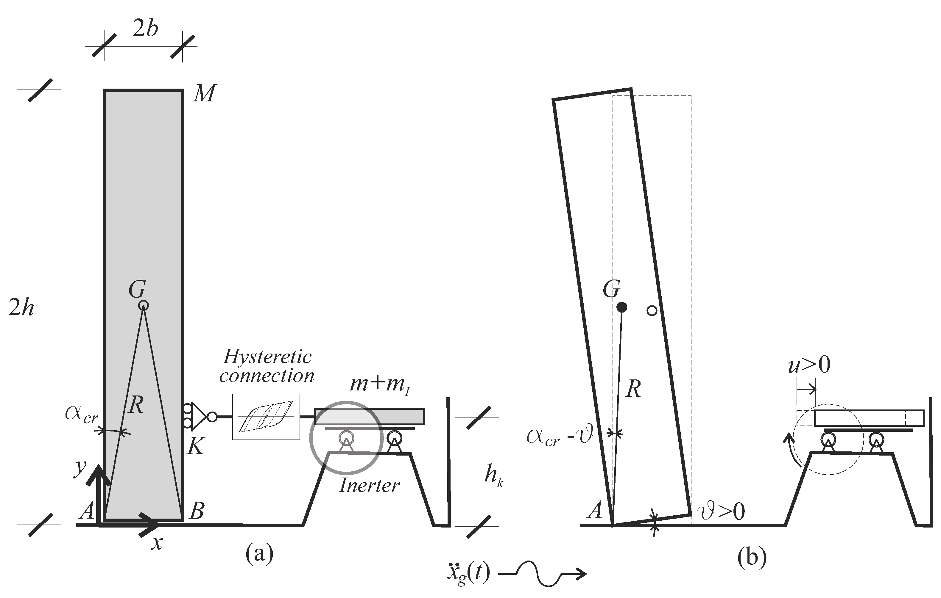
Figure 2.
Rack–pinion–flywheel supplemental rotational inertia system.

Figure 3.
Frequency–response curves of coupled systems (thick lines) and stand-alone rigid blocks (thin lines) for different values of the post- to pre-yielding stiffness ratios and different values of the apparent mass . Points A–D: points used in further analyses. Dimensions of the rigid block: and (, ).
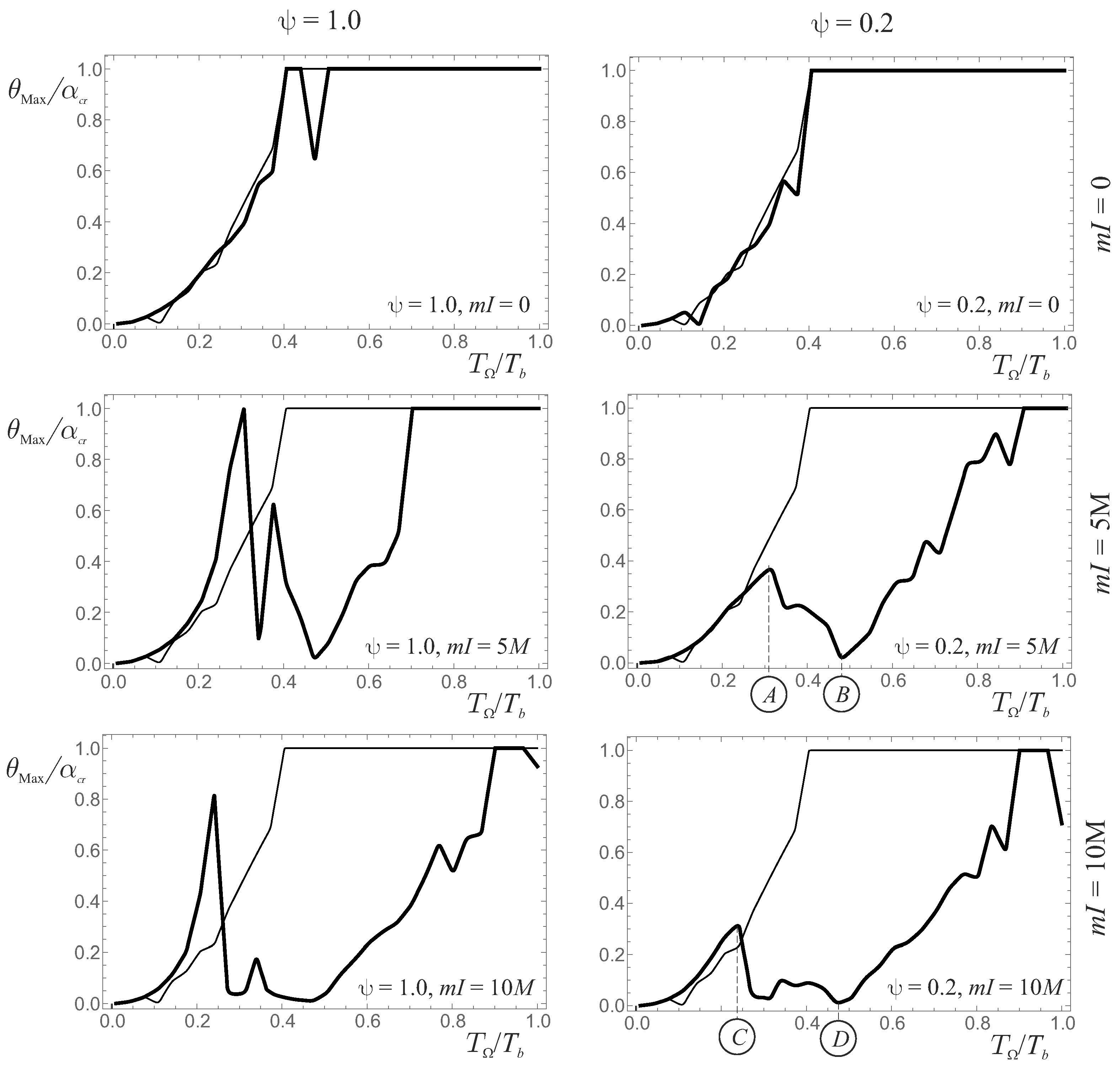
Figure 4.
Time histories of the displacements (thin lines) and (thick lines): (a) Time histories for coupled systems defined by points A and B of the frequency curve of Figure 3 (); (b) Time histories for coupled systems defined by points C and D of the frequency curve of Figure 3 (). Dimensions of the rigid block: and (, , ).
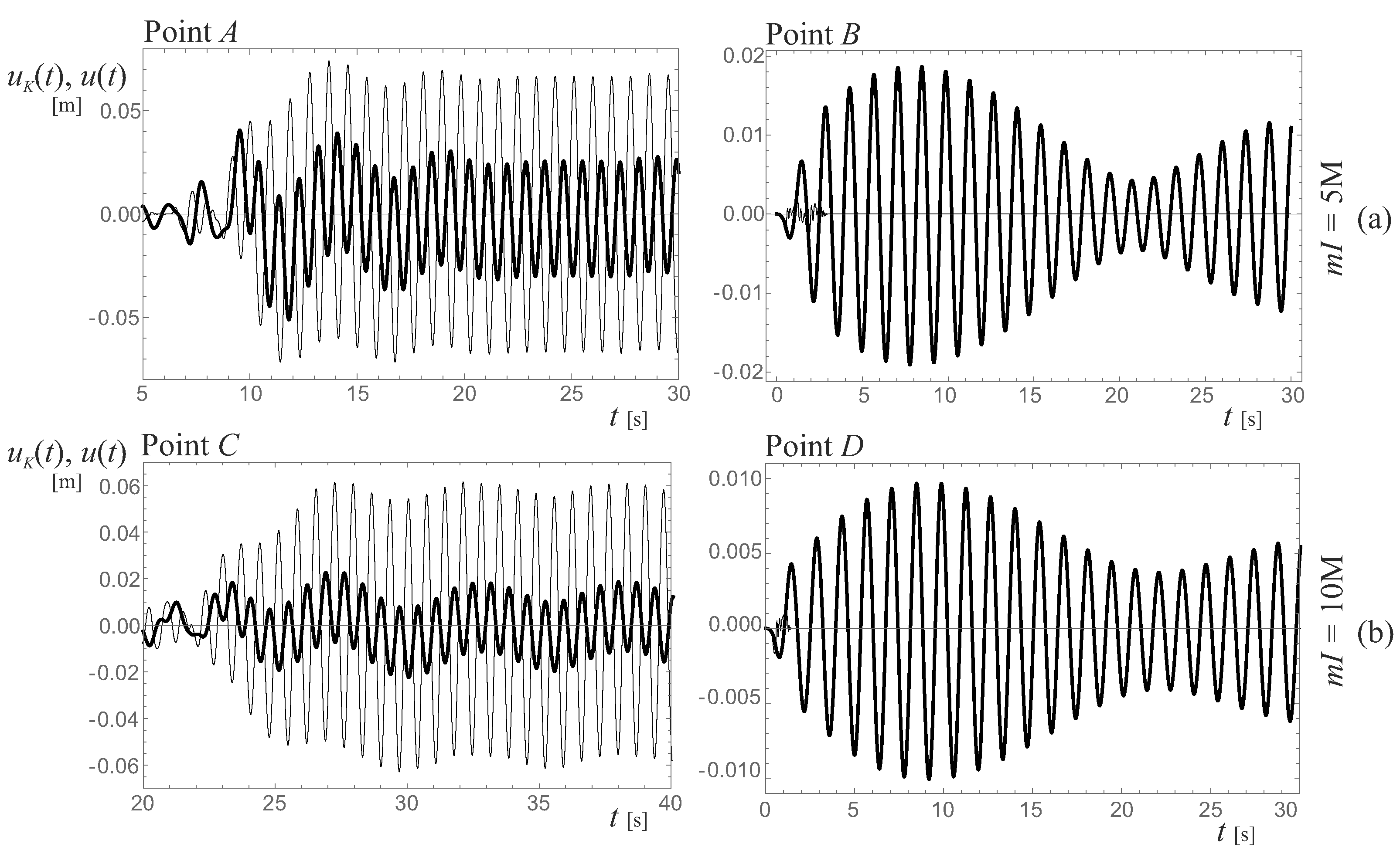
Figure 5.
Frequency–response curves of coupled systems (thick solid and dashed lines) and corresponding stand-alone rigid blocks (thin lines): (a) curves for different apparent masses (); (b) curves for different yielding displacements (); (c) curves for different physical masses m (). Dimensions of the rigid block: and ().
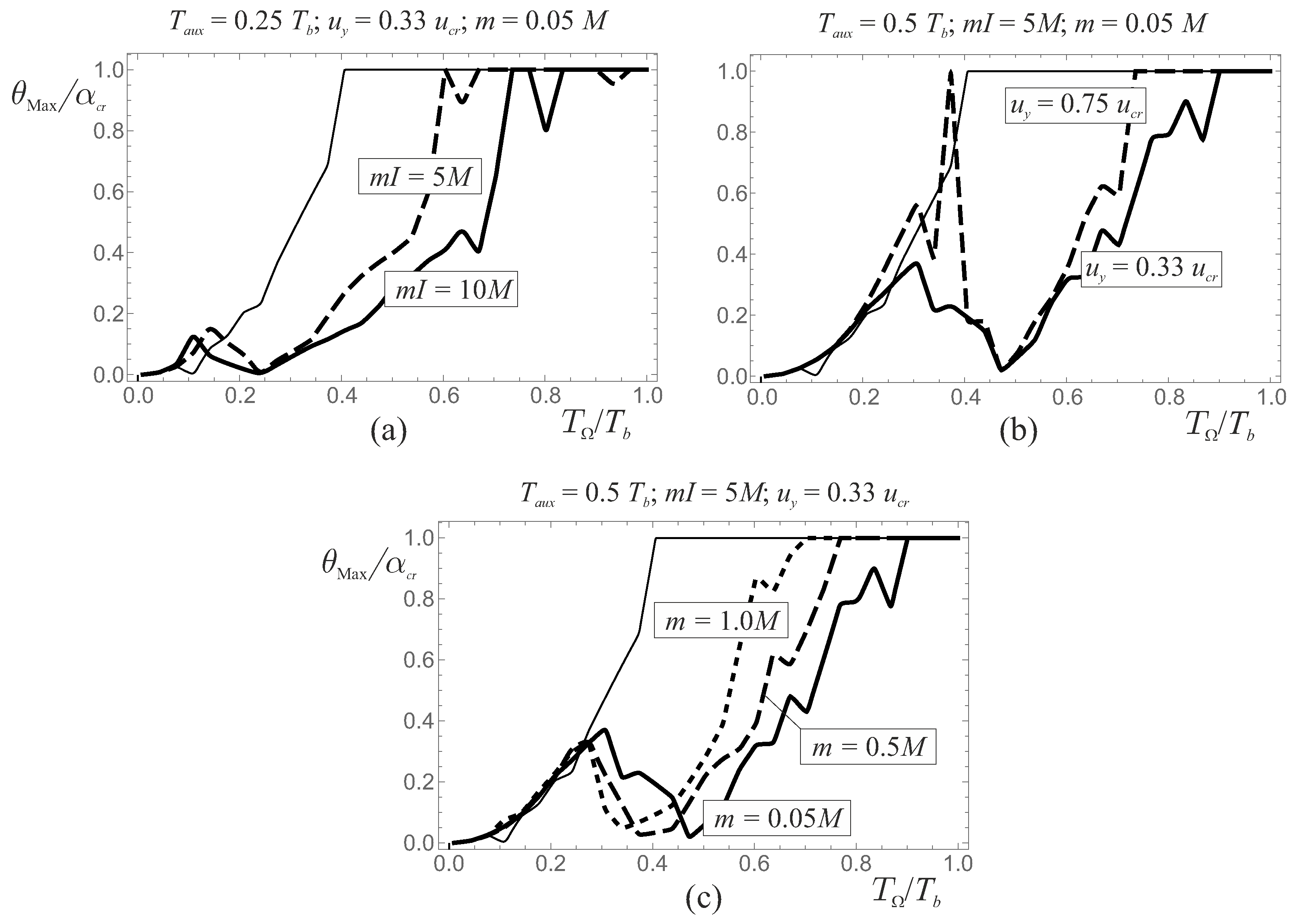
Figure 6.
Frequency–response curves of coupled systems (thick solid and dashed lines) and corresponding stand-alone rigid blocks (thin lines): (a) curves for different apparent masses and dimensions of the rigid block and (); (b) curves for different apparent masses and dimensions of the block: and (), ().

Figure 7.
Time histories and pseudo-acceleration spectra of the earthquakes analysed: (a) Kobe; (b) L’Aquila; (c) Newall; (d) Christchurch.
Figure 7.
Time histories and pseudo-acceleration spectra of the earthquakes analysed: (a) Kobe; (b) L’Aquila; (c) Newall; (d) Christchurch.
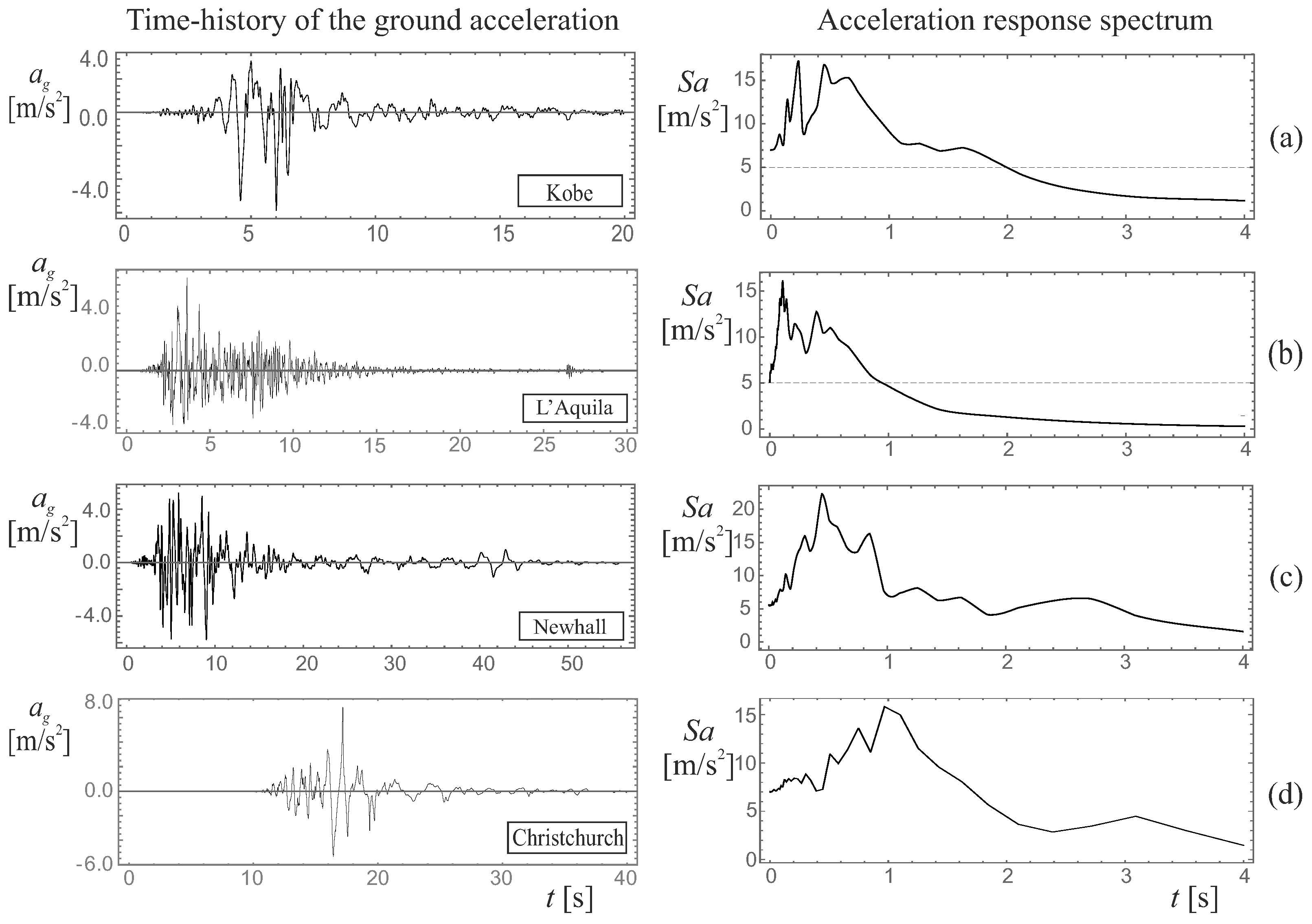
Figure 8.
Gain surfaces (top graphs) and maps (lower graphs) for the Kobe seismic record: (a) dimensions of the rigid block and (); (b) dimensions of the rigid block and (), ().
Figure 8.
Gain surfaces (top graphs) and maps (lower graphs) for the Kobe seismic record: (a) dimensions of the rigid block and (); (b) dimensions of the rigid block and (), ().

Figure 9.
Frequency–response curves of the coupled systems (thick lines) and stand-alone rigid blocks (thin lines): (a) curves evaluated for coupled systems defined by points , and C of Figure 8b; (b) curves evaluated for coupled systems defined by points A and D of Figure 8b. Dimensions of the rigid block: and (, ).
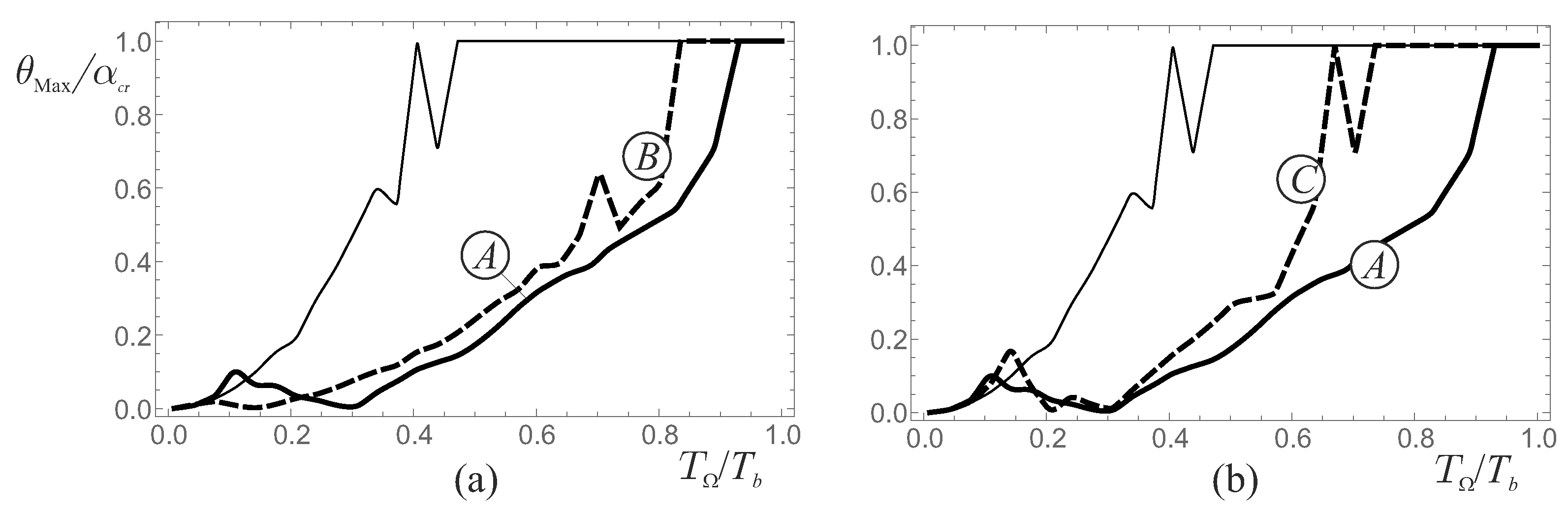
Figure 10.
Time histories of the displacements (thin lines) and (thick lines) for coupled systems defined by points E and F of Figure 8a. Dimensions of the block: and (, ).
Figure 10.
Time histories of the displacements (thin lines) and (thick lines) for coupled systems defined by points E and F of Figure 8a. Dimensions of the block: and (, ).
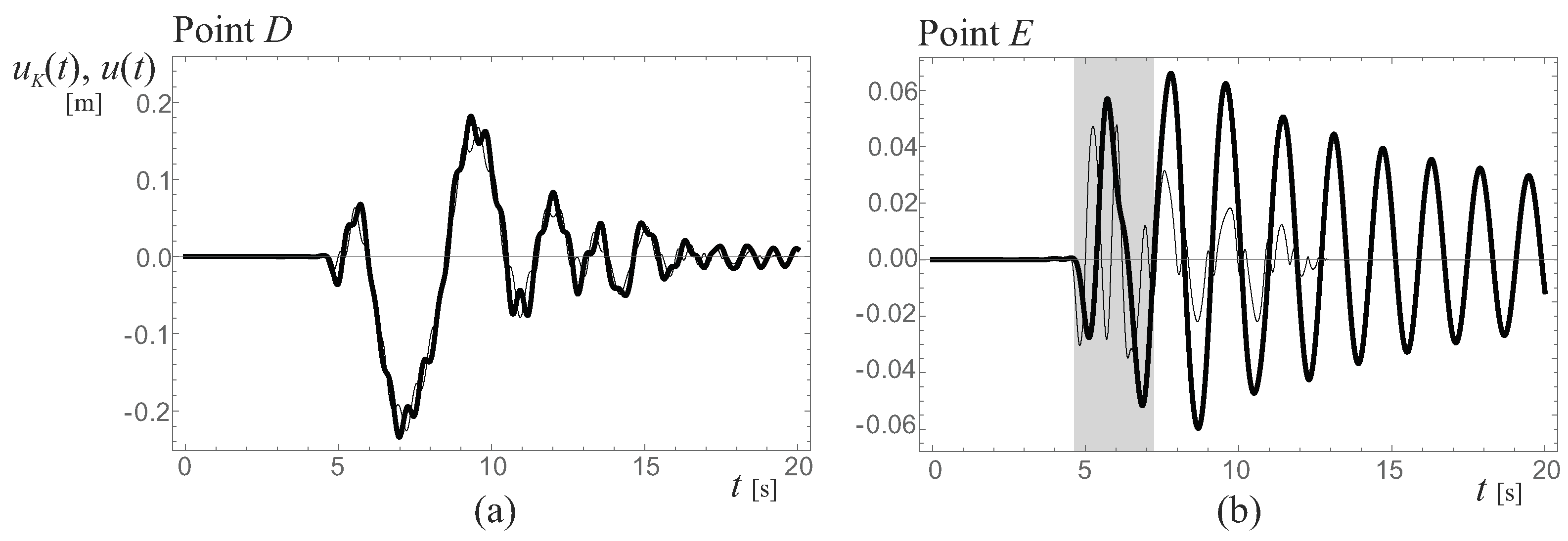
Figure 11.
Gain maps obtained for different dimensions of the rigid blocks and under the L’Aquila seismic record ().
Figure 11.
Gain maps obtained for different dimensions of the rigid blocks and under the L’Aquila seismic record ().

Figure 12.
Comparison between the response spectrum of the seismic records (upper graphs) and the frequency–response curves of coupled systems with rigid blocks of dimensions and (lower graph): (a) Kobe seismic record; (b) L’Aquila seismic record (, ).
Figure 12.
Comparison between the response spectrum of the seismic records (upper graphs) and the frequency–response curves of coupled systems with rigid blocks of dimensions and (lower graph): (a) Kobe seismic record; (b) L’Aquila seismic record (, ).
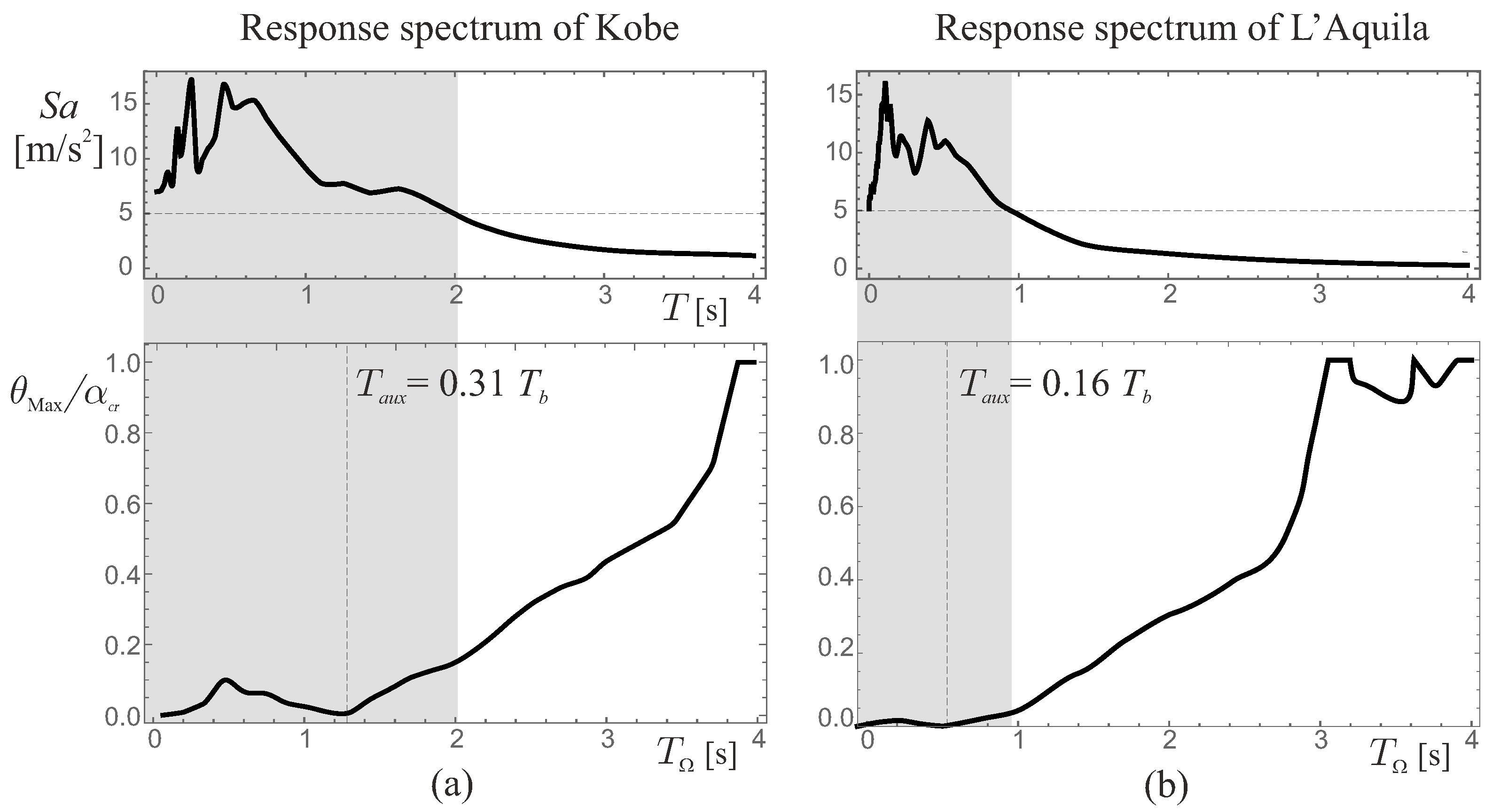
Figure 13.
Gain maps obtained for different dimensions of the rigid blocks and under the Newhall seismic record ().
Figure 13.
Gain maps obtained for different dimensions of the rigid blocks and under the Newhall seismic record ().
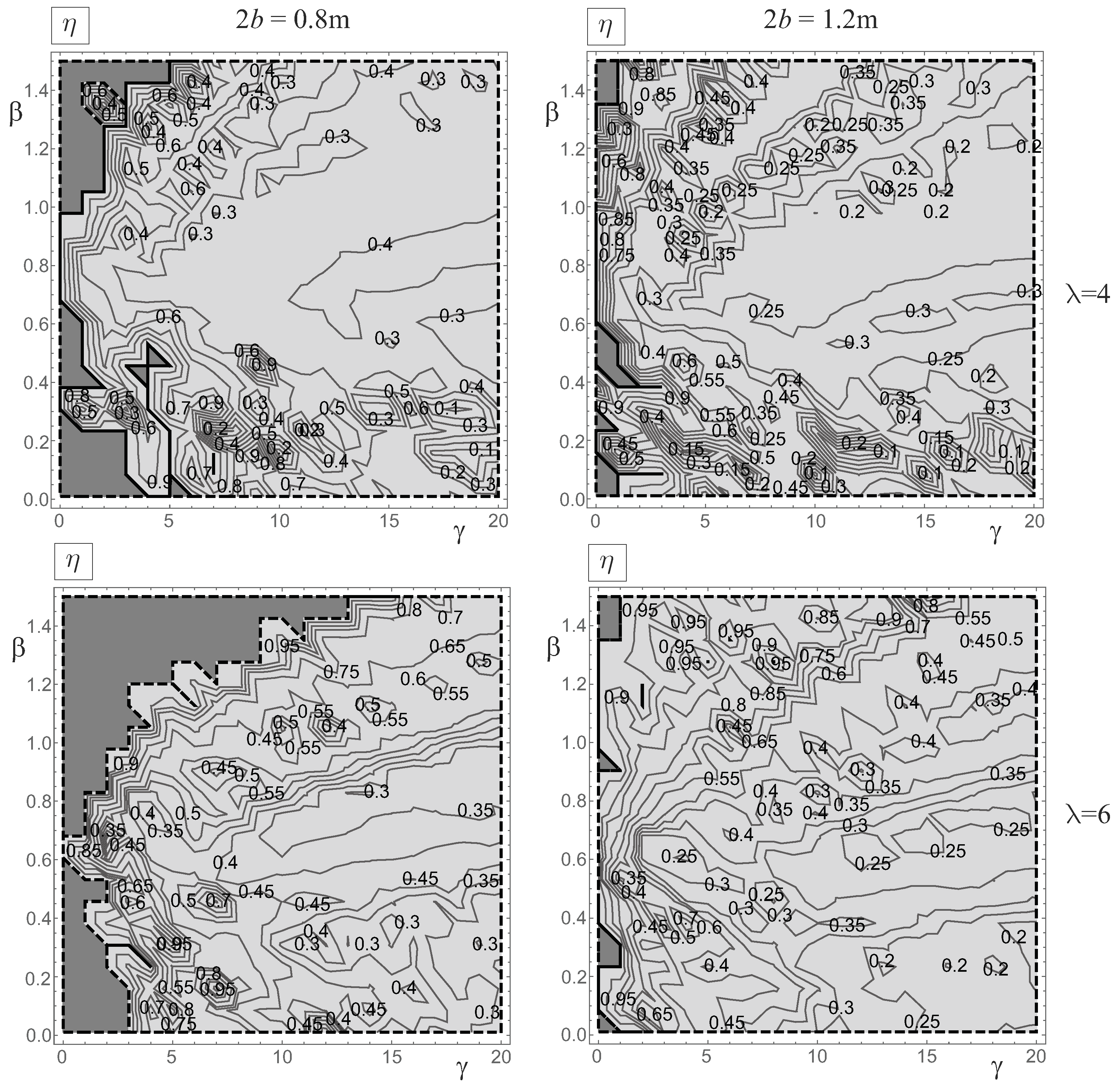
Figure 14.
Gain maps obtained for different dimensions of the rigid blocks and under the Christchurch seismic record ().
Figure 14.
Gain maps obtained for different dimensions of the rigid blocks and under the Christchurch seismic record ().

Publisher’s Note: MDPI stays neutral with regard to jurisdictional claims in published maps and institutional affiliations. |
© 2022 by the authors. Licensee MDPI, Basel, Switzerland. This article is an open access article distributed under the terms and conditions of the Creative Commons Attribution (CC BY) license (https://creativecommons.org/licenses/by/4.0/).
Share and Cite
MDPI and ACS Style
Di Egidio, A.; Contento, A. Improvement of the Dynamic and Seismic Behaviour of Rigid Block-like Structures by a Hysteretic Mass Damper Coupled with an Inerter. Appl. Sci. 2022, 12, 11527. https://doi.org/10.3390/app122211527
AMA Style
Di Egidio A, Contento A. Improvement of the Dynamic and Seismic Behaviour of Rigid Block-like Structures by a Hysteretic Mass Damper Coupled with an Inerter. Applied Sciences. 2022; 12(22):11527. https://doi.org/10.3390/app122211527
Chicago/Turabian StyleDi Egidio, Angelo, and Alessandro Contento. 2022. "Improvement of the Dynamic and Seismic Behaviour of Rigid Block-like Structures by a Hysteretic Mass Damper Coupled with an Inerter" Applied Sciences 12, no. 22: 11527. https://doi.org/10.3390/app122211527
Note that from the first issue of 2016, this journal uses article numbers instead of page numbers. See further details here.