Article

Competition in a New Industrial Economy: Toward an Agent-Based Economic Model of Modularity

1
Department of Industrial Economics, Tamkang University, Tamshui, New Taipei City 251, Taiwan
2
AI-Econ Research Center, Department of Economics, National Chengchi University,Taipei 116, Taiwan
*
Author to whom correspondence should be addressed.
Adm. Sci. 2014, 4(3), 192-218; https://doi.org/10.3390/admsci4030192
Submission received: 28 February 2014 / Revised: 4 June 2014 / Accepted: 18 June 2014 / Published: 4 July 2014
(This article belongs to the Special Issue Computational Organization Theory)

Abstract

:
When firms (conglomerates) are competing, not only for the present, with a given population of customers and a fixed set of commodities or service, but also for the future, in which products are constantly evolving, what will be their competitive strategies and what will be the emerging ecology of the market? In this paper, we use the agent-based modeling of a modular economy to study the markup rate dynamics in a duopolistic setting. We find that there are multiple equilibria in the market, characterized by either a fixed point or a limit cycle. In the former case, both firms compete with the same markup rate, which is a situation similar to the familiar classic Bertrand model, except that the rate is not necessarily zero. In the latter case, both firms survive by maintaining different markup rates and different market shares.

1. Introduction

1.1. Overview of the Research

In this paper, we investigate the evolution and heterogeneity of commodities from a quality perspective. Therefore, it is critical to have an abstract representation of this evolutionary process, i.e., a representation of commodities and their changes over time. Conventional economic theory, which is very much quantity-oriented, does not offer a quality-oriented representation of commodities and the changes therein, so we resolve this by using a modular representation. (Some earlier related works using a different representation, namely, Kauffman’s NK landscape model, will be briefly reviewed in Section 1.3.)
This modular representation was inspired by Herbert Simon’s work on near decomposability or modularity [1]. Modularity refers to a structural relationship between a system as a whole and the constituent components, which can function as independent entities. It is a key to harnessing a possibly unbounded complex system. Simon [1] was probably one of the most influential pioneers inspiring many follow-up works in various scientific disciplines [2]. (Simon may never have used the term modularity, while his notion of near decomposability was frequently renamed modularity in the literature [3], and Simon did not seem to object to this different name [2]. Of course, one has to pay particular attention to the fine difference between the two. In particular, modules, as manifested in many concrete applications, may be viewed as only parts of near-decomposable systems. They serve as the elementary units, which are fully decomposable and fully encapsulated and upon which near decomposable (weakly-interacting) systems can be built.) In addition to near decomposability, Simon viewed hierarchy as a general principle of complex structures. He advocated the use of a hierarchical measure—the number of successive levels of hierarchical structuring in a system—to define and measure complexity; furthermore, he argued that hierarchy emerges almost inevitably through a wide variety of evolutionary processes, for the simple reason that hierarchical structures are stable.
Our modular representation naturally allows for a hierarchical representation of a commodity, which can then explicitly manifest the quality of the commodity (see Section 1.2 for an illustration). The hierarchical modular representation of a commodity can be interpreted as an explicit layout of a production process, which combines various raw and intermediary materials using different processors at different stages and at different times.
In order to understand the changes in the hierarchical-modular commodities in a dynamic context, we will need the fundamental driving force from the demand side. This requires us to have a preference and utility theory that is compatible with the hierarchical representation of the commodity. Not surprisingly, the quantity-oriented microeconomic theory does not leave room for such a development. We need to search for a new foundation for the evolutionary process of the hierarchical products.
It turns out that, to have a compatible preference theory, we also need a modular representation of preferences. The assumption that preferences also have a hierarchical modular structure is less evident than that for a commodity. While modularity in the brain and mind has recently been extensively studied [4,5,6,7,8,9], whether the claim of a modular brain or mind implies the claim of a modular preference is still an issue to be addressed. Without empirical grounds, [10] proposed three conditions required for a well-behaved modular preference: monotonicity, synergy and consistency [10]. If the preference can be given a modular structure, then the utility of consuming a specific commodity can be calculated using the module matching algorithm, which we propose in this stage of the research. Furthermore, the aforementioned synergy condition can lead to a utility function, which has increasing marginal utility in quality. This last property seems to be the backbone of the value-added-oriented service economy.
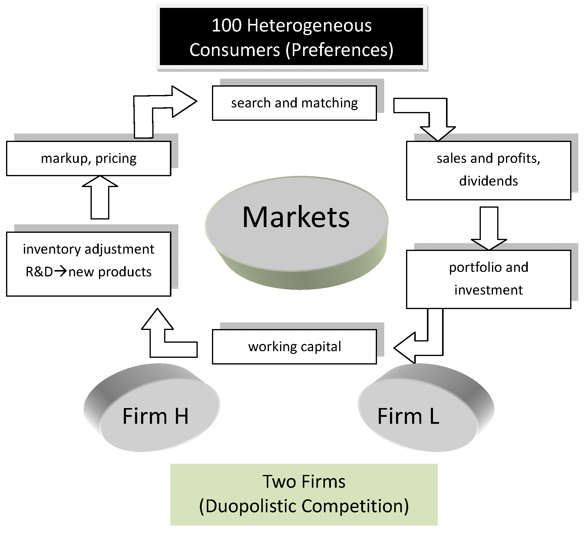
The next two elements are firms that produce these commodities and the markets where demand meets supply. In addition to product diversification, the firms in this modular production framework need to decide on product quality (the hierarchical content of the commodity) and the efforts devoted to the development of new products. Without R&D, the above choices become rather superficial; therefore, the searching behavior (R&D) for new and good products also becomes a transparent part of the model. In this stage, our demand-supply model (a market model) of a quality-oriented economy is ready, and we call it the modular economy.
Technically, the modular economy relies on a formalization quite different from the ones used in conventional mathematical economics. Rather than real analysis, this new formalization relies more on formal language theory, such as context-free grammar, and combinatorics. (The representation of the preference and the production (commodity) space can be constructed using the theory of formal languages, for example, the Backus–Nauer form (BNF) of grammars invented by John Backus (1924–2007). The class of languages described by the BNF, including recursively defined non-terminals, is equivalent to the context-free languages (Chomsky’s Type 2 languages). The well-known Chomsky hierarchy of languages, established by Noam Chomsky, has four types of languages. From the languages generated by the very restricted grammars to those generated by the unrestricted grammars, there are the regular languages (generated by the regular grammars), the context-free languages (by the context-free grammars), the context-sensitive languages (by the context-sensitive grammars) and the recursively enumerable languages (by the unrestricted grammars). The one generated by the more restricted grammars is a proper subset of the one generated by the less restricted grammars. In addition, based on the languages that can be accepted or recognized, there is a corresponding hierarchy of automata: the finite state automata (accepting the regular languages), the pushdown automata (the context-free languages), the linear bounded automata (the context-sensitive languages) and the Turing machines (the recursive enumerable languages). In other words, the commodities and the preferences operated in this paper are those that can be accepted by the pushdown automata. We can certainly consider the higher classes as a future direction for research. For the details of these technical backgrounds, the interested reader is referred to [11].) Specifically, the evolutionary process of the commodities in the modular economy (the searching process for new and good-quality products) is realized through genetic programming [12,13].
To see whether we can gain some insights from the operation of the modular economy, the aforementioned modular economy is applied to the study of price competition or non-price competition. We begin this study with a duopolistic competition market [14]. There are two firms; each one applies a uniform markup rate to set the prices of all of the products they supply. One firm adopts a high markup rate and the other adopts a low markup rate. The research aims to see whether price competition is critical for the firms’ survival in this duopolistic competition. Through multiple runs (100 runs) of the simulation, we find that the high markup firm has competitive superiority as compared to the low markup firms. Out of these 100 runs, the high markup firm actually drives out the low markup firm 50 times, while the process also takes place in the other direction 37 times. Despite the lack of the overwhelming dominance, the result is counterintuitive, because, in a weak sense, it has violated the law of one price, or at least people would expect the result to be expressed the other way round.
Based on their observation of the simulations, Chie and Chen [14] proposed one explanation for this puzzling result. Basically, in the modular economy, the competition among firms does not just proceed in a horizontal way, but more in a vertical way. The sophisticated products (the more hierarchical ones) may be the substitutes for the less sophisticated products (the less hierarchical ones) if the former can match the consumers’ modular preference at a higher level. In this case, the former can generate a larger synergy effect than the latter and, hence, can provide consumers with a higher utility. Nonetheless, to successfully develop this product, the firm needs a higher markup in order to generate enough revenue for R&D. Although this may not explain the whole story in the complex evolving economy, it provides the basic justification for the survival of the high markup firm with the presence of the low markup firm as its rival.
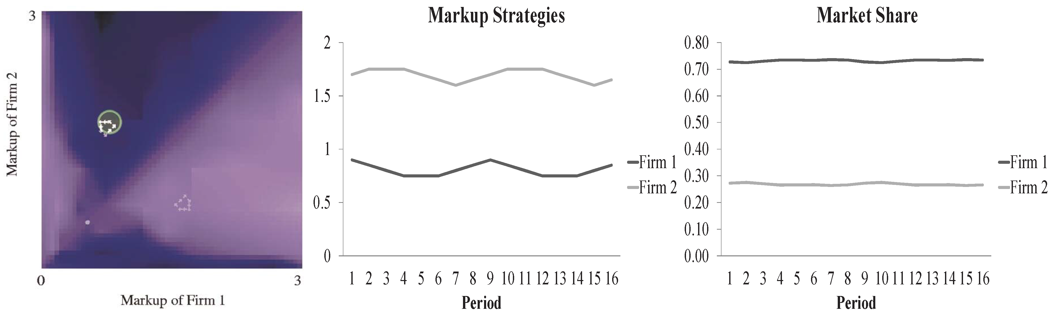
In this paper, we extend the simulation model in Chie and Chen [14]. While the previous study shows the superiority of a high markup strategy, the simulation was performed with a fixed pair of markups. In a more realistic setting, the firm may change its markup rate in response to its competitor’s strategy under the survival pressure. This may trigger further reactions of the rival firm. This chain of reactions can lead to different sorts of dynamics as the outcome, and it is not clear 
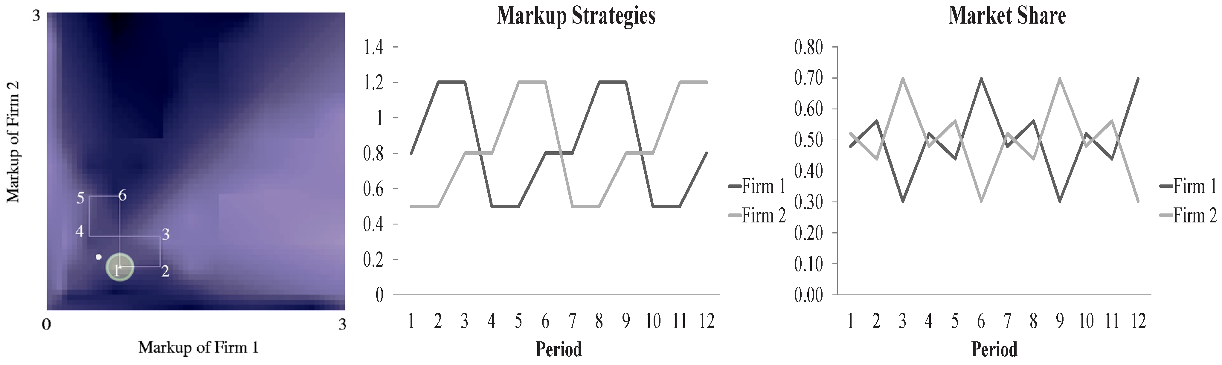
a priori which one will emerge. Would there be a fixed point in the end, so that only one markup can exist in the market and the law of one price is saved in this sense? Or, would there be limit cycles or strange attractors, so that the differences in markups can persistently exist? These are the issues that this paper shall address. Our contribution is to show the possible attractors of the co-evolving markup dynamics, which shed light on the interesting patterns observed in the empirical IO literature [15,16,17,18]. For that purpose, we also give some thought to the discovered attractors. In sum, this work extends Chie and Chen’s model [14] by allowing the dynamically evolving markups and then examines the role of price in duopolistic competition.
The rest of the paper is organized as follows. In Section 1.2, we use the evolution of the mobile phone to motivate the idea of the modular economy. We then present in Section 2 the agent-based modular economy of duopolistic competition. Simulation designs are presented in Section 3, followed by the simulation results and their analysis (Section 4). Finally, Section 5 provides the concluding remarks.

1.2. Hierarchical Representation of the Evolution of Mobile Phones

To motivate the idea of the modular economy, we use the well-known example of the mobile phone. 
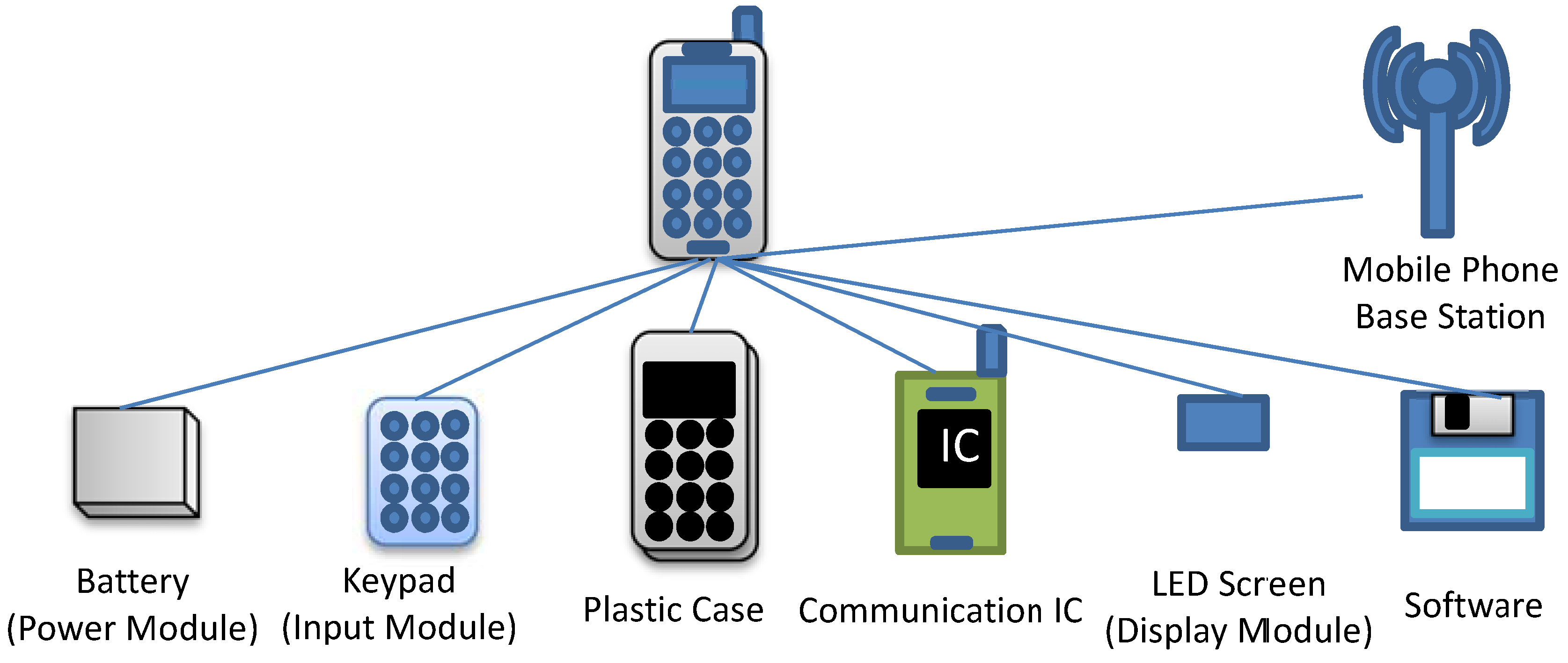
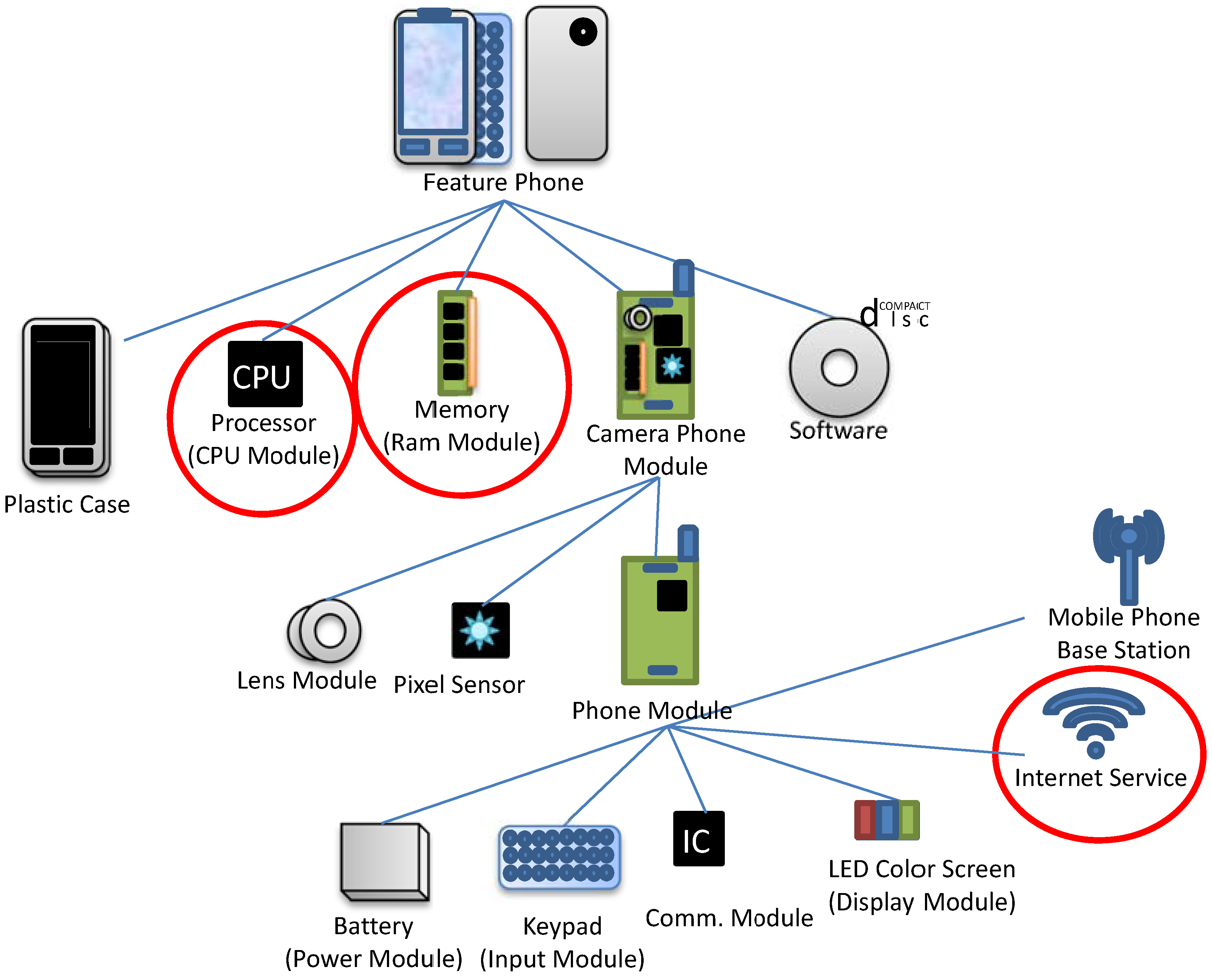
Figure 1 shows the constituent modules of a mobile phone. The battery (power model), keypad (input model), plastic case, communication IC and LED screen (the display module), shown at the bottom of Figure 1, are considered to be the encapsulated (internal) modules and the base station (connecting or networking module) to be an internal module. One form of the evolution of the mobile phone is that one or many of its modules undergo a “mutation”. For example, in 
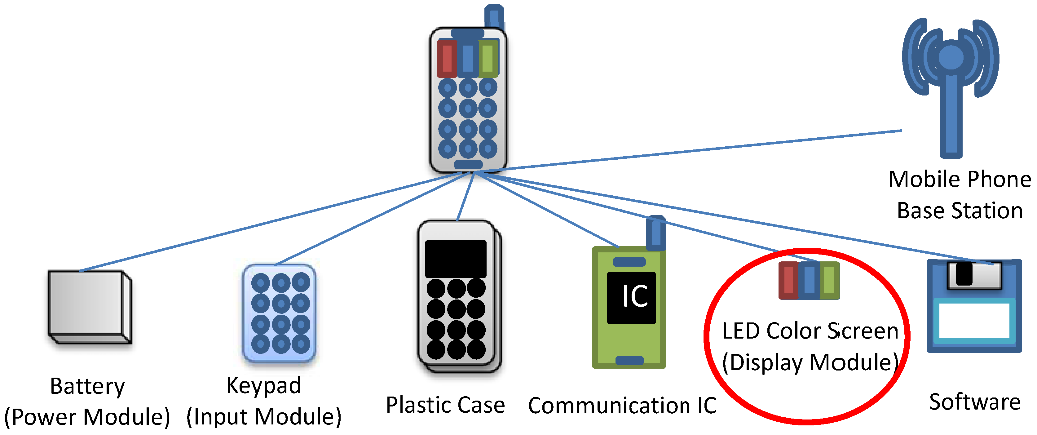
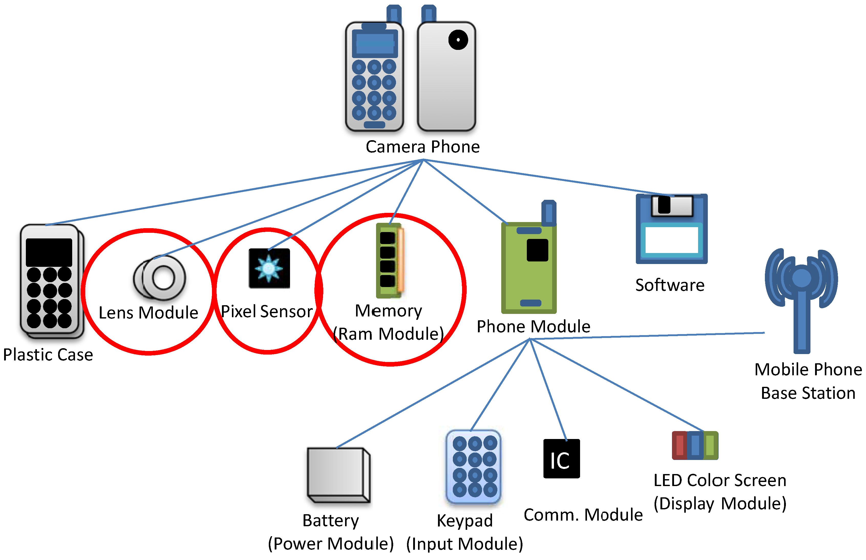
Figure 2, a “mutation” occurs in the display module; the original black-and-white display screen is replaced by a color screen. Then, a new product emerges. At this point, the mobile phone is still just a phone. As time goes by, some modules evolve into independent modules of a two-level hierarchy and work with another independent module (camera). This synergy takes place by incorporating into the mobile phone a number of the conventional camera modules, including a lens, pixel sensor, and memory, as shown in Figure 3. Now, we have a new product, the camera phone, a product with three levels of hierarchy, as shown in Figure 3. Next, this camera phone serves as another independent module and is integrated with a module known as the “assistant” or “secretary” module, which has the submodules of, for example, CPU and RAM (
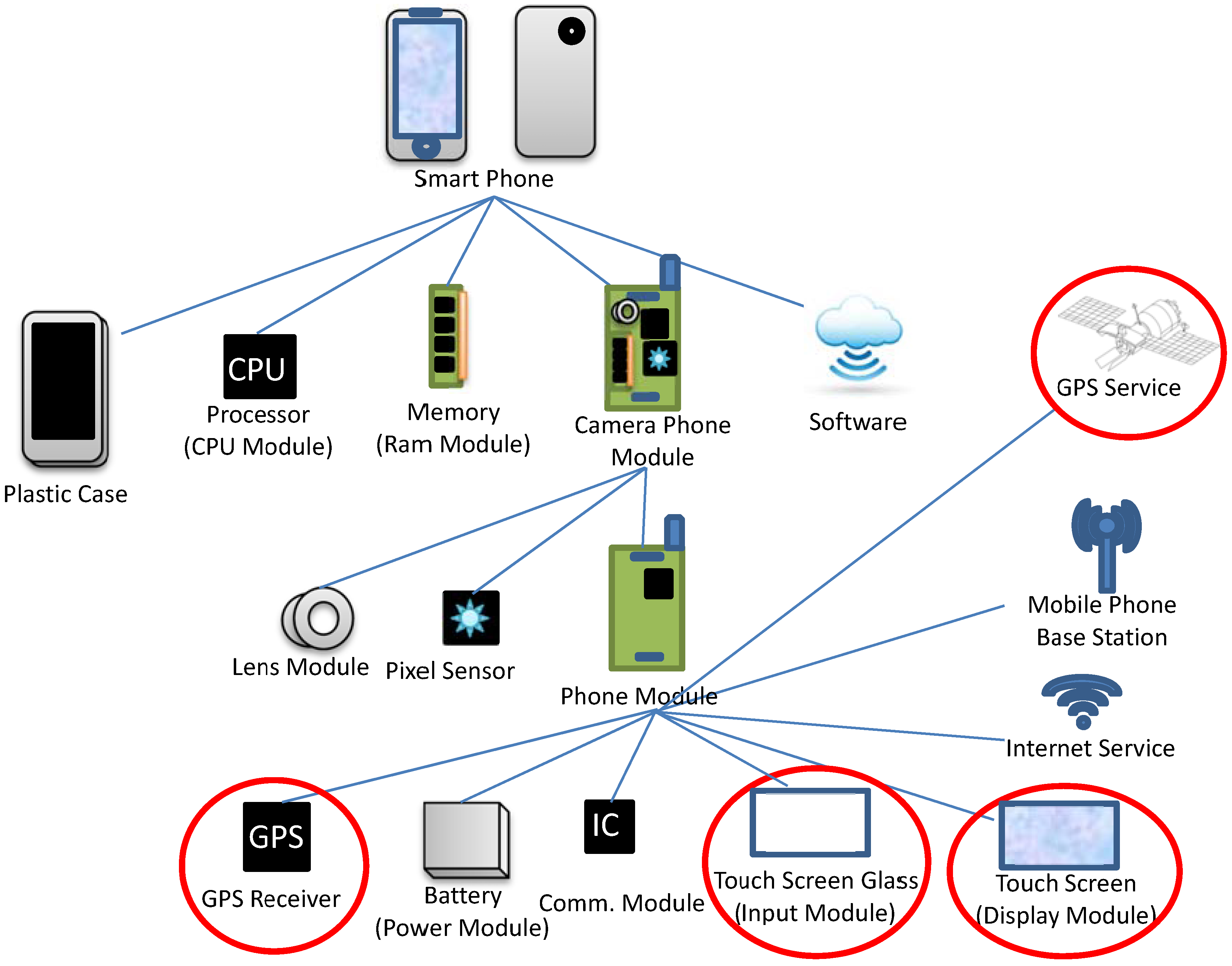
Figure 4). Then, this integration is accompanied by another indispensable independent module, namely, the Internet service. As a result, a new product with four levels of hierarchy, known as the PDA phone or the feature phone, emerges. In the final stage of this example, a number of the constituent modules of the feature phone are enhanced. The input module is upgraded to touch screen glass and the display module is upgraded to a touch screen. The further additions of a GPS receiver as an internal module and the GPS service as an external module make the feature phone become a smart phone (Figure 5).
Figure 1. Mobile phone: black and white.
Admsci 04 00192 g001
Figure 2. Mobile phone: color.
Admsci 04 00192 g002
Figure 3. Camera phone.
Admsci 04 00192 g003
Figure 4. Feature phone.
Admsci 04 00192 g004
Figure 5. Smart phone.
Admsci 04 00192 g005
Figure 1, Figure 2, Figure 3, Figure 4 and Figure 5 give an overview of the evolution of the mobile phone, specifically expressed in terms of hierarchical modularity. The description may be rather casual, but the message delivered is quite clear. Modularity becomes the essential element that one cannot afford afford to miss, if one wants to have a reasonable representation of the evolution of the economy in terms of what is produced. A more abstract or general presentation of the evolutionary process is drawn in Figure 6.
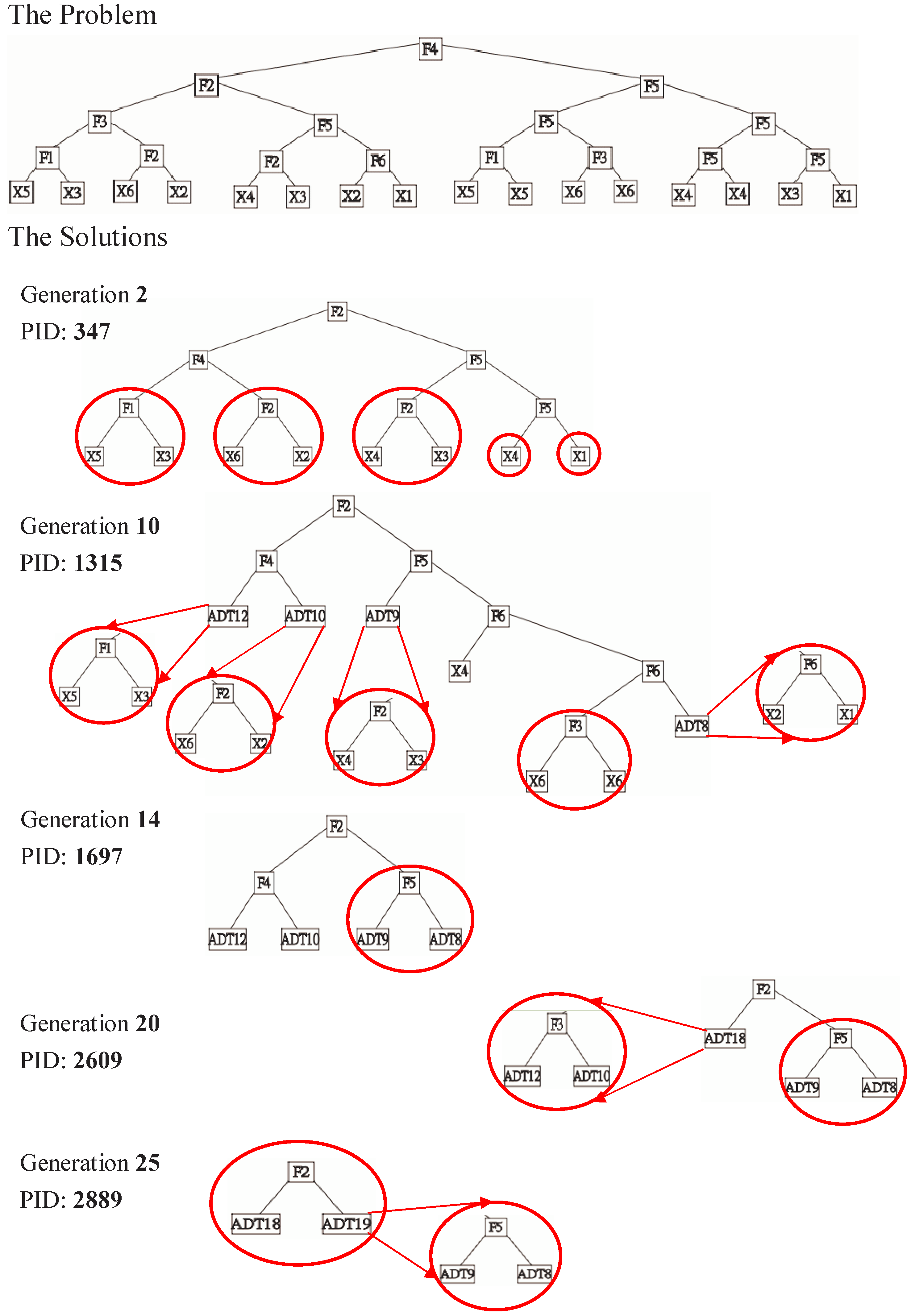
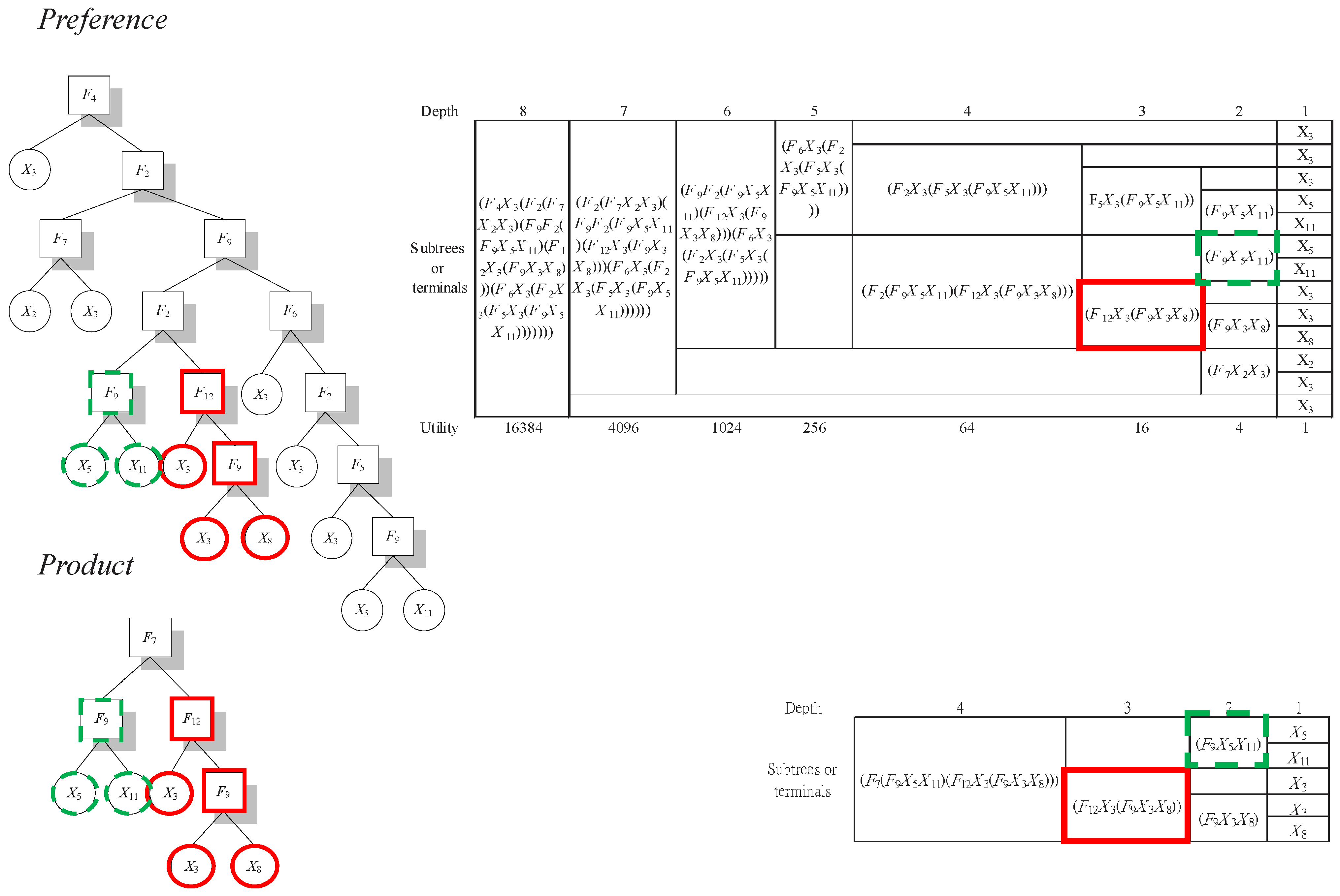
What appears at the top of Figure 6 is the parse-tree representation of a consumer’s preference, which introduces the “problem” for producers. The whole parse tree corresponds to a word generated by recursively applying a number of production rules from a context-free grammar. Each of its subtrees is also a word, but with less deep recursion. The shallowest recursion is just the application of a single production rule: null →x, where x∈Σ and Σ is the terminal set. All of the nodes at the bottom of the tree, also called leaves, are this kind of shallowest recursion. The deeper the recursion, the bigger the subtree, and the complete tree involves the largest number of recursions compared to all of its subtrees. This recursive structure denotes the modular structure of a preference, from a very primitive preference with shallow recursion to a complex preference with deep recursion. It also indicates the growing and evolving nature of a preference.
As seen in Section 2.3 and Table 1, a power utility function will be used to represent this modular preference. The power utility function is used mainly for the purpose of satisfying the synergy condition (other specifications that satisfy this condition can also be employed). Taking the mobile phone as an example, the synergy effect means that the utility of a camera phone is greater than the sum of the utility of a phone and the utility of a camera. Of course, in the real economy, we would not expect this assumption to hold true for all consumers over all commodities. In other words, consumers are heterogeneous in their modular preferences (the preferences of consumers are randomly generated, and the degree of the heterogeneity of their preferences is directly controlled by the number of distinctive elements in the function set and the terminal set (to be given in Table 1)). That is, the synergy effect applies to each consumer in different ways. Hence, camera phones may have the synergy effect for some consumers, but not for all; likewise, smart phones may have the synergy effect for some consumers, but not for all.
Figure 6. Hierarchical representation of the evolution of an artificial commodity.
Admsci 04 00192 g006
Table 1. The parameter settings.
ParameterType (Variable)RangeValue
Producer
Number of FirmsInteger ( N p )[1, ]2
Initial Working CapitalInteger ( K 0 )[0, ]100 × B( N i , 0.5)
Inventory Adjustment RateReal (λ)[0, 1]80%
Markup RateReal (η)[0, ]Figure 7
R&D RateReal ( γ R D )[0, 1]1%
Retained EarningsInteger ( R E m i n )[0, ]500
Consumer
Number of ConsumersInteger ( N c )[1, ]100
Base of the Power Utility FunctionReal[2, ]4
Consumer Income per PeriodInteger (I)[1, ]10,000
Search IntensityReal ( γ s )[0, 1]100%
Investor
Number of InvestorsInteger ( N i )[1, ]100
Initial BudgetInteger ( B 0 )[1, ]1,000
Probability of ZIStrategyReal ( p Z I )[0, 1]20%
Reinvestment RatioReal (α)[0, 1]80%
Investment CeilingInteger[0, ]2000
Time Schedule
Number of Rounds per Trading DayInteger (R)[1, ]5
Number of Trading DaysInteger (T)[1, ]5,000
Genetic Programming
Size of Terminal SetInteger[1, ]5
Size of Function SetInteger[1, ]5
Crossover RateReal ( p c )[0, 1]90%
Mutation RateReal ( P m )[0, 1]80%
Tree Mutation RateReal ( P t m )[0, 1]50%
B( n , p ) is the binomial distribution with n trials and success probability p.
Notice that the consumer himself may not know his own preference ex ante. In this case, the preference is revealed only up to the extent that there is a product that matches the preference. This has been shown in the sequence of diagrams below the consumer’s preference (tree). In each of these diagrams, one can see that a number of products, circled in red, have been successfully developed to match some subtrees of the whole preference. In this case, only these parts of the preference (the matched ones) are revealed.
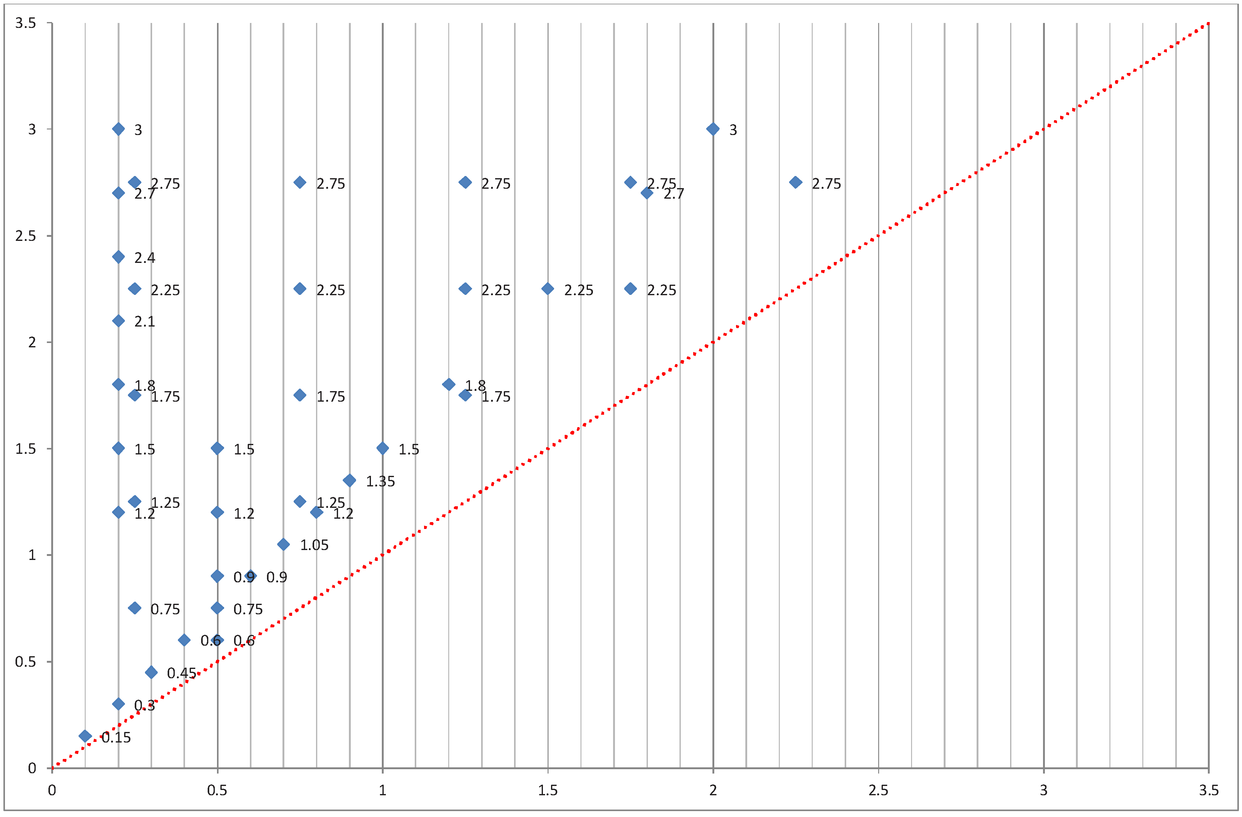
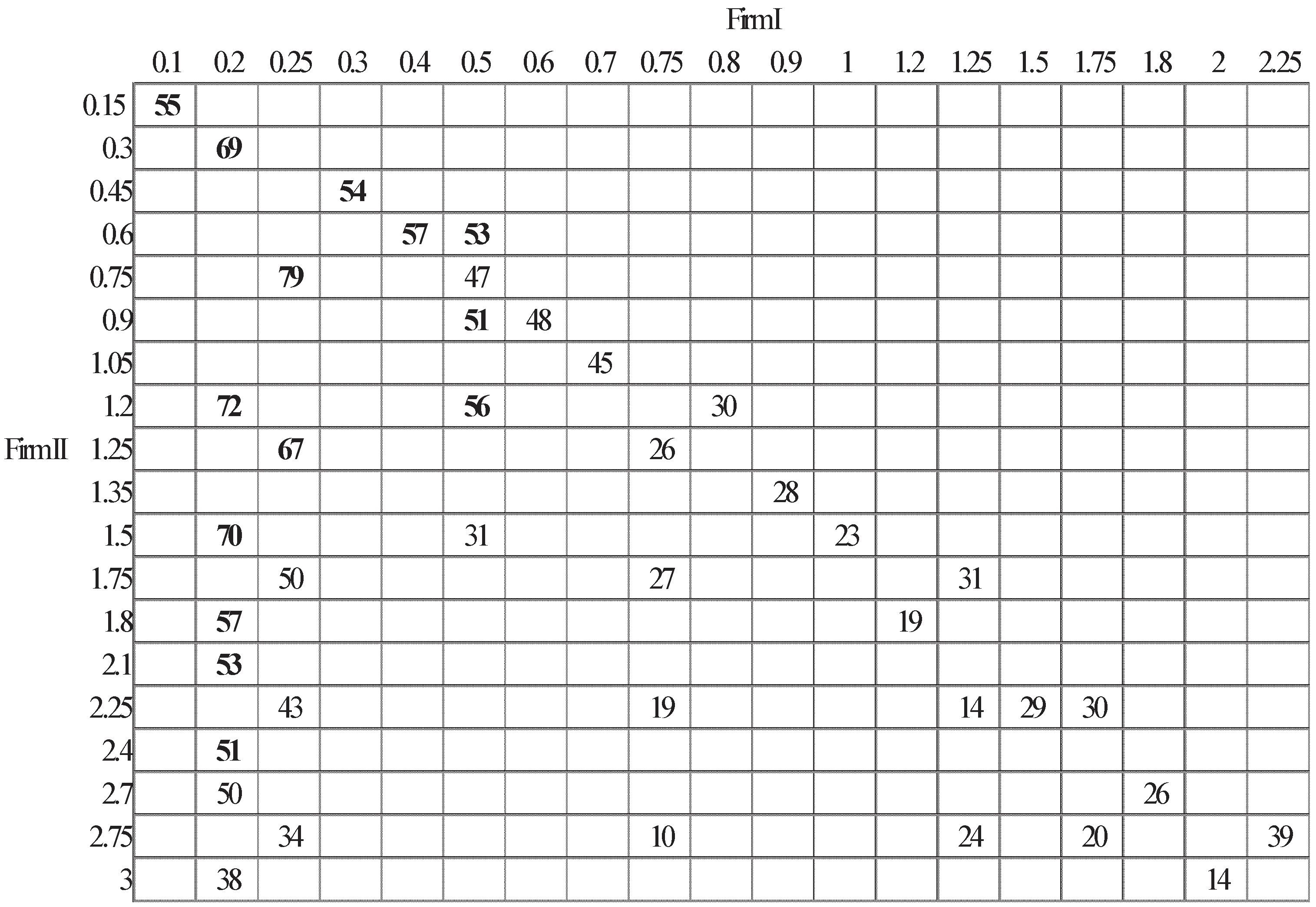
Figure 7. Simulation designs: 40 pairs of markup rates.
Admsci 04 00192 g007

1.3. A Brief Remark on the NK Model

The general analytical or computational model, which is able to demonstrate the evolutionary process, as demonstrated in Figure 6, is very limited in the literature. Based on Frenken [19], the only available alternative is Kauffman’s NK model [20,21]. (For a general review of the agent-based computational models of innovation, the interested reader is referred to Dawid [22]. However, Dawid [22] does not include the work on the NK model. In a separate article appearing in the same volume, Chang and Harrington [23] did give a review of the relevance of the NK models in the evolution of organizations.) In the NK model, the features or modules of a product, i.e., N, and the possibility of their interactions, i.e., K, are given exogenously. The evolution of the product can then be perceived as the optimal design to combine these features or modules. Various search algorithms have been proposed to find the optimal design over the landscape [20,21,24,25]. The search process itself can then be perceived as an evolutionary process.
We consider this class of models as a good starting point to approach Simon’s idea of the complex system, i.e., near-decomposable system. We, however, are not satisfied with the NK landscape model due to the following two conceptual limitations. First, the space to embed the evolutionary process as demonstrated in Figure 6 should, in principle, be infinite-dimensional rather than finite-dimensional. For example, it would be inconceivable to think of the evolution from the DOS system to the Windows system as just the fine-tuning of some parameters in a finite-dimensional space. Second, the features (modules) of a product in general should be part of the evolutionary process and emerge out of the process rather than being exogenously given. As in the mobile phone example, the number of features changes over time when the mobile phone evolves into the smart phone.
Technically speaking, the NK model normally represents a product with a fixed-length string with a fixed set of alphabets. This representation can capture the ideas of the modularity, but not the hierarchical ones. Our proposed tree representation is equivalent to the string representation, but with variable lengths [26]. Therefore, the tree model is more general than the string model and can work well with the idea of the hierarchical modularity. Less formally, the evolutionary search and discovery process should include both what we know we do not know (known unknowns) and what we do not know we do not know (unknown unknowns). The NK model is more suitable for the former, but not the latter. However, for those who are familiar with Hugo in Simon’s famous story of Apple [27], the real-life scenarios are filled with a series of unknown unknowns. Apple, as Simon described, is a non-technical version of [27].

2. An Agent-Based Modular Model of Duopolistic Competition

2.1. An Overview

Before discussing the operational details of each agent (firm, consumer and investor), we first give an overview of the flow of the model. The dynamics of the model can be regarded as a cycle, as shown clockwisely in Figure 8. Each trading day, date t, starts with consumers entering the market (Section 2.3). Each trading day is composed of a number of trading rounds. In each trading round, the consumers enter the market by following a randomly determined sequence. In each round, the consumers shop around the market to obtain the commodity that can satisfy them most in terms of the consumer’s surplus given their budget constraints. After all of the rounds in a market day, the consumers leave with a basket of commodities, which, conditional on their budget constraints, is in a sense satisficing. The sales and profits of each product are then determined by the consumer’s choices (Section 2.2). Based on the profits gained and the firm’s dividend policy, each firm pays dividends to its investors (Section 2.2 and Section 2.4). After receiving the profit statistics and the dividends, the investors invest in each firm according to their portfolio decisions (Section 2.4). The investment and the retained earnings become the firms’ working capital on which all operating budgets are based. The firms will then make their resource-allocation decisions and distribute the working capital, minus the desired retained earnings, between inventory replenishment and R&D. The R&D will lead to some novel designs of products, which, with the inventory, will result in a new set of products. Based on the firm’s marketing strategy, this new set of products will be post-priced to be sold to the market on the next trading day. Then, the clock ticks, and trading day t + 1 starts.

2.1.1. Trading Institution

The trading institution is a posted-price menu system. No bargaining or auction is considered as a possible trading protocol in this paper. All commodities produced at the end of the last market day will be listed in the menu at the beginning of this market day. Consumers shop around and decide their priorities according to the menu (see also Section 2.3.1). If the commodity in which a consumer is interested is sold out, the consumer will move to the next affordable commodity on his priority list. He will constantly shop, until his list is exhausted or the market is closed. The aggregate demand of each commodity is the sum of all of the orders for that commodity, denoted by d i , t . Of course, only when the demand is less than the supply x i , t 1 can all consumers be satisfied. Nonetheless, based on d i , t , the firm can re-adjust its production plan at the end of the market day (see more in Section 2.2.1).
Figure 8. An overview of the market cycle.
Admsci 04 00192 g008
In this specific demonstration, the market scale is characterized by 100 consumers (households) and two firms.

2.2. Firms

In the typical setting of a perfectly competitive economy, where products sold in the market are homogeneous, price is the only key factor to distinguish between winners and losers. The firms with cost advantages survive. This is the typical lesson taught in rather static economic theory. In a more practical and dynamic business world, firms can compete for consumers’ interests via various strategies. In addition to pricing, they can resort to product differentiation, branding, customer relationship management, cost control and innovation. These strategies, in a simpler version, can be roughly categorized into production (including R&D), marketing and finance. Section 2.2.1 and Section 2.2.3 will detail the first two dimensions, and Section 2.2.2 will provide the details of the last.
It is worth mentioning that firms have to compete not only in the product market, but also in the capital market. Firms seek to have good market performance by introducing favorable products into the market, so that they can attract more capital injections from investors. Given that consumer preferences are difficult to delineate, high market performance would not be possible without the continuous involvement of R&D, which, in turn, requires funding resources. Hence, Section 2.2.1, Section 2.2.3 and Section 2.2.2 are closely tied together.

2.2.1. Production and Sales

Commodity Initialization When a commodity is randomly generated (discovered) by R&D, only one unit is produced initially. Since the development of a new product is a trial-and-error process, this setting allows the firms to use their limited working capital to have a larger exploration of the diversity of the commodities.
Production In each period t, a firm’s production is constrained by its total working capital at that time ( K t ). Working capital is first used to replenish the inventory of the existing products according to the re-adjusted production plan made at the end of the previous market day. This process is known as inventory adjustment. The speed of inventory adjustment is based on the given inventory adjustment rate (λ). After making such an inventory adjustment, a firm will use the residual working capital to develop new products through R&D to explore consumer preferences at a higher level. The extent of the residual capital devoted to R&D, γ R D , will determine the scale of the exploration. Although R&D can lead to a greater variety of firms’ products, it can be risky, since new products can fail badly. Putting these items together, the production activities of a firm can be represented by the correspondence (1):
F : ( K t , λ , γ R D ) { x i , t } , i = 1 , . . . , N t ; t = 0 , 1 , . . . , T 1
Here, N t is the number of different products supplied by the firm at time t, and x i , t is the quantity of the i-th product.
Marketing and Sales Pricing or the markup rate is part of a firm’s marketing strategy. This markup rate coupled with the production at the end of the current trading day will partially determine the sales in the next period, which is represented by Expression (2).
M : ( η , x i , t ) { s i , t + 1 } , i = 1 , . . . , N t ; t = 1 , . . . , T 1 ; s i , t + 1 x i , t
In this paper, the markup rate (η) is considered to be a constant applied over the entire set of products and throughout the whole simulation horizon; hence, we do not use the more specific notation, η i , t . The quantity of product i sold at time t is denoted by s i , t , which is to distinguish it from the monetary sales, denoted by S i , t .
Given the triplet ( λ , γ R D , η), the production, marketing and resource allocation of a firm can be described as follows. For each market day t, the firm will begin with the replenishment of the goods sold on the last market day, t 1 . The reproduction of each existing commodity will be based on the inventory policy (λ) and its demand. More specifically,
x ^ i , t = x i , t 1 + λ ( d i , t x i , t 1 ) , i = 1 , 2 , . . . , N t 1
where d i , t is the quantity of commodity i demanded on market day t. (In this model, the unit of commodity can only be an integer; therefore, what Equation (3) actually does is to round off x i , t if it is fractional. Once this fine adjustment becomes clear, we shall not further complicate the notation and shall use x i , t throughout the paper.) We assume that all commodities are perishable, so Equation (3) is not just about the desirable inventory level, but also the desirable production level. Of course, whether the firm is actually able to have enough capacity to fulfill all of its planned production depends on its working capital K t . The firm is, therefore, assumed to fulfill its planned production up to its capacity limit, and it will produce x i , t sequentially, from one, two, ..., up to the largest i * ( 1 i * N t 1 ), such that:
K t i i * C i ( x ^ i , t ) 0
where C i refers to the total cost of producing x i , t ; C i ( 0 ) = 0 for all i. By the constraint (4),
x i , t = x ^ i , t , if   i i * 0 , if   i > i *
If i * = N t 1 , then all planned production will be realized.
In addition to the existing commodities i = 1 , . . . , N t 1 , in each period of time, the firm will also allocate a portion of its working capital to R&D in order to develop new products. By the R&D policy ( γ R D ), let:
K t R & D = ( K t i = 1 N t 1 C i ( x i , t ) ) × γ R D
The firm will then use K t R & D to produce a series of new products, each initially with one unit, also sequentially up to a maximum number Δ N t 1 , such that:
K t R & D i Δ N t 1 C i ( x i , t ) 0
The number of commodities produced by the firm is now updated to N t , where N t = N t 1 + Δ N t 1 . The firm then sells { x i , t } ( i = 1 , 2 , . . . , N t ) in the market on the next market day t + 1 and, by the marketing policy (η), acquires the monetary sales S i , t + 1 on the next market day for each commodity i ( i = 1 to N t ),
S i , t + 1 = s i , t + 1 × [ ( 1 + η ) × c i ( x i , t ) ] , s i , t + 1 = min { x i , t , d i , t + 1 }
where s i , t + 1 is the quantity of the product i sold on market day t + 1 and c i ( x i , t ) is the average cost of producing x i , t .

2.2.2. Working Capital

The difference between total sales and total costs is the profits earned by the firm in period t. Alternatively,
π t + 1 = i = 1 N t S i , t + 1 i = 1 N t C i ( x i , t )
The profit will then be distributed to the firm’s investors as dividends ( D t ), based on their investment share and based on the firm’s dividend (or retained earnings) policy, i.e.,
D t + 1 = max { 0 , R E t + π t + 1 R E m i n }
where R E m i n is the minimum retained earnings that the firm would like to keep for the purpose of cushioning, and R E t is the retained earnings carried over from the last period (period t), which is the undistributed earnings after taking into account production, R&D and dividends. After receiving the dividends, the investors can decide their re-investment in the firm, based on its performance (see Section 2.4). Denote the total investment that the firm receives from the investors at time t + 1 by I t + 1 . The dynamics of the working capital is given in Equation (11).
K t + 1 = ( K t i = 1 N t C i ( x i , t ) ) + i = 1 N t S i , t + 1 D t + 1 + I t + 1 = ( K t i = 1 N t 1 C i ( x i , t ) p r o d u c t i o n i = N t 1 + 1 N t C i ( x i , t ) R & D ) + i = 1 N t S i , t + 1 D t + 1 + I t + 1 = R E t + i = 1 N t S i , t + 1 D t + 1 + I t + 1
By Equation (10), if D t + 1 is positive, we then have for K t + 1 at least a minimum of R E m i n . A pseudo code for the full cycle of a market day is given as follows:
Admsci 04 00192 i001

2.2.3. R&D

R&D is the sole source of new products and is implemented by genetic programming [12,13]. Since all products are represented by parse trees, their generations and alterations can be operated through genetic programming using the standard operators, including random initialization, crossover and mutation, as shown in Figure 9. Genetic programming starts with some primitives, divided into the terminal set and the function set, which, in our application, corresponds to the set of raw materials and the set of processors. The function set is fixed, but the terminal set adapts to the market dynamics. New terminals (new modules) are found through pattern searching, which is to identify the common part (the common subtree) of the successful products. These terminals, also called the automated defined terminals (ADTs), will then be used in the genetic alteration (mutation) of the existing products.
Figure 9. Genetic programming as an engine for R&D.
Admsci 04 00192 g009

2.3. The Consumers

2.3.1. Search

On each trading day, each consumer will enter the market in an order randomly determined. Each consumer will then decide what to place in his basket through searching (shopping). How extensively he will search depends on a parameter’s search intensity ( γ s ), which is exogenously assigned to each consumer. The search intensity then determines the fraction of sellers the consumer can reach. For example, if the search intensity is 50%, then the consumer will reach half of the sellers in the market. If there are two sellers, then the consumer will visit one of the two.
Without losing generality, consider now that the j-th consumer enters the market. He visits a number of firms determined by his search intensity. For all firms that he visits, he examines all commodities in the menu (Section 2.1.1) and calculates the consumer’s surplus for each commodity, i.e., the difference between the highest willingness to pay and the actual price paid. The highest willingness to pay is measured by the utility that the consumer will have by consuming the product (the algorithm is to be detailed in Section 2.3.2). Then, he ranks the commodities from the one with the highest consumer’s surplus to that with the lowest and picks those with the highest surplus subject to his budget affordability. He then leaves the market, and the j+1th consumer enters the market, repeating the same procedure. After all consumers finish their shopping, this shopping round ends, and the next shopping round begins. After a number of consecutive shopping rounds, a market day is over, and the calendar moves to the next market day.

2.3.2. Preference Matching

To calculate a consumer’s surplus and to form his preference list require a matching between the modules of the consumer’s preferences and the modules of the commodities. A module matching algorithm is proposed to tackle this issue. The module algorithm applied in our modular economy is satisfied by the following two principles: maximum matching and double-counting avoidance. The former indicates that we start the match with the largest module (the deepest hierarchical tree), then the second, then the third, and so on, until there is no more match. The latter means that any part of the module that has already been matched should not be included in the subsequent matches. In this way, the module algorithm is compatible with the quality-based economy, which reflects the increasing marginal utility in quality. An illustration of this match algorithm is shown in Figure 10. In this example, the exemplar consumer has two matched models, which leads to a total utility of 20. (Here, a power function with a base of four is applied. The choice of this parameter is, however, rather flexible, as long as the synergy condition can be satisfied [10].) By equating the cost of the product to its product complexity or the number of nodes, we calculate the cost of the product to be nine. Let us say that if the posted price is 10, by considering a 11% markup, then the consumer’s surplus for this production is then 10 (=20 − 10).

2.4. The Investors

In each period of time (on each trading day), each investor will decide in which firm to invest and will invest in one and only one firm. This discrete decision is made under two types of investment behavior. The first kind involves the zero-intelligence investor, who basically throws a fair coin to decide in which firm to invest. The second kind is the myopic best-response investor, who decides in which firm to invest in a stochastic manner. The probability of choosing a firm is proportional to the rate of return of each firm in the previous period. (This linear probability rule can be applied to the cases where both firms have either positive or negative rates of return. However, when one firm has a positive return and one firm has a negative return, we assume that the myopic best-response investor will only be interested in the firm with positive returns.) Each investor will behave by following these two modes of behavior stochastically. The chance to behave randomly is parameterized by p Z I , and the chance to behave more rationally, therefore, is 1 p Z I . This simple design is mainly to relate investment motives to profits and treat the mixture of all other motives as noisy behavior. There are, of course, many variations in this design, and we will not fully exploit other possibilities in this paper, but will leave them to subsequent studies. (For example, we are thinking of how this model can be applied to the study of the behavior of the venture capital industry in light of empirical data.)
Figure 10. Preference matching.
Admsci 04 00192 g010
The tree in the upper left panel refers to the modular structure of a consumer’s preference, and the tree in the lower left panel refers to the modular structure of the product to be evaluated by the respective consumer. By following the module matching algorithm, the first largest module matched is marked in red and the second largest one is marked in green. Other than these two, there is no further match. Hence, the utility that the consumer can gain from this product is the sum of these two modules, i.e., 20 (=42 + 41). The right part of the figure provides a list of all modules used to constitute the preference (upper right) and the product (lower right). Various possible modules are arranged by the depth (level), from the highest (the most sophisticated) to the lowest (the most primitive).
The size of the investment depends on the investors’ total available endowment accumulated up to the last period, B t 1 , starting from an initial endowment B 0 . This endowment will be divided into two parts, one for investment and one simply for hoarding or for future investment. In this article, we consider a fixed proportion between the two, and let the parameter α be the proportion for investment; hence 1 α is the proportion for hoarding.
We also calibrate an investment upper ceiling for each investor. This ceiling is set to avoid the overproduction of the current economy. The overproduction can occur, because the number of consumers is exogenously fixed in this economy, which inevitably leads to an upper bound for the total feasible expenditures. Of course, this artificial constraint can be removed in a general equilibrium model, where investors and consumers are given a one-to-one correspondence, and a higher accumulated endowment naturally leads to higher purchasing power. Nevertheless, a general equilibrium approach to the modular economy is more demanding, and hence, only a partial-equilibrium approximation is made in this paper.

3. Simulation Design

The main focus of this paper is on the co-evolutionary competitive dynamics when both firms are assumed to be myopic best-response to their market shares and both employ the markup rate as the only control variable. Since the two firms differ in terms of their products supplied, a comprehensive market share covering all products sold will be used. Let S t j be the total sales of firm j in period t ( j = 1 , 2 ).
S t j = i = 1 N t 1 j S i , t j
The market share of firm j in time period t, m k t t j , is:
m k t t j = S t j S t , j = 1 , 2
where:
S t = j = 1 2 S t j
To carry out the analysis, we shall use the model proposed in Section 2 to generate a lookup table. (The assumption of the availability of the lookup table is equivalent to assuming that both firms can actually use the agent-based duopolistic model established in Section 2 to generate the required statistics for decision support. In a real situation, they may not be able to obtain access to this “perfect” model. In that case, we need to model their adaptive dynamics in the setting of markup rates. Hence, the simplification via using a lookup table is mainly for the purpose of having a theoretical underpinning before we move into the possible learning dynamics. Having said that, we shall leave the learning dynamics to a further study.) The lookup table, T , basically informs the firm of its long-term average market share if its own markup rate is η i and the rival firm has a markup rate η i , i.e.,
T ( η i , η i ) ( m k t i , m k t i ) , η i , η i Λ
where Λ is the strategy space.
We start with a two-dimensional strategy space bounded below by zero and above by three; hence Λ × Λ = ( 0 , 3 ) × ( 0 , 3 ) , as shown in Figure 7. The choice of this range is based on a large body of empirical studies on markups, from sectors to individual firms [28,29,30,31]. Based on these empirical studies, a range from zero to two should be sufficient. Nevertheless, given that the firms studied in this paper are conglomerates with both innovation and multi-products, the conventional estimation based on single-product firms at a high level of aggregation may not entirely represent the tail behavior of the markup distribution. Hence, we enlarge the upper limit of the range from two to three.
From this strategy space, we then take a finite sample of the pair of strategies (markup rates) adopted by the two firms. Since the payoff matrix should be symmetric, we only need to sample the pairs exclusively, either above the 45-degree line or below the 45-degree line. We specifically sample the pairs above the 45-degree line, so that the y-axis represents the rate of the high markup firm and the x-axis represents the rate of the low markup firm. As shown in Figure 7, we have a total of 40 samples on this half space. The 40 samples also cover the one specifically used in [14, i.e., the pair (0.10, 0.15), as indicated at the southwestern corner of the space. In this specific case, Chie and Chen [14] showed the superiority of the high markup firm over the low markup firm in terms of both market share and profit.
In this study, we have extended the original study to include another 39 pairs of marketing strategies (markup rates) and examine how far the superiority of the high-markup firm (the H firm for short) can go. As an extended study, the rest of the parameters are set to be the same values as those in [14], and they are summarized in Table 1. Simulations are run using the software, ModularEcon, which is available on the website of the open source codes for agent-based modeling [32].
The software is written using Java and is compiled by Borland J Builder 6. It is implementable under the DOS environment. Parameters are specified in the file innvo.ini, whereas innvo.jar is the execution file. Various outputs regarding households and firms are written in the Excel files. As a simulation of the evolution of the economy, the modular economy is very computationally demanding. Depending on the given complexity of consumer preferences and the endowment, it may take an Intel Core i5 4-core processor 10 h for a run with 5,000 market days.

4. Results and Discussions

In Figure 11, we present the market share of the H firm. The number shown in each cell is the average market share, averaged over a number of 50 runs of the same scenario, each run lasting for 5,000 periods. From the figure, we can see that the high markup rate as a competitive strategy has its limit. However, the pattern revealed in Figure 11 is not monotone. Specifically, when the markup rate of the rival firm is fixed at a low level, i.e., below 50%, the competitive advantage of the H firm features a hump shape, in the sense that the market share of the H firm will increase first with its markup rate, up to a point, and then decrease when the markup rate is further increased. This hump shape then seems to be replaced with a monotone decreasing curve when the markup rate of the low firm is fixed at a higher level.
Figure 11. Market share of the high markup firm under different pairs of strategies.
Admsci 04 00192 g011
To study the possible long-term competitive dynamics, we first use both interpolation and extrapolation to gauge the possible market share of each firm under a total of 3,600 ( 60 × 60 ) markup rates. We then take this complete table as a payoff matrix (the lookup table) for both firms and assume that each firm reacts to the other firm’s strategy in the best response manner by following the lookup table. There are two possible schedules for this interaction. One is under the assumption that the firms react in a sequential way, so that the two firms move in turn, and at each point of time only one firm moves. The other one is based on the assumption that they both move simultaneously. Not too surprisingly, these two schedules may lead to different limit points, as shown in Figure 12.
Figure 12. Domain of attraction: sequential move (left) and simultaneous move (right).
Admsci 04 00192 g012
The myopic sequential dynamics shows the convergence to one fixed point and one limit cycle. Hence, there are multiple equilibria characterized by a steady-state markup rate, which is 60% in this case, and a cycling fluctuation of markup rates, as also shown in Figure 13. To show which is more likely, we also color each attractor’s domain of attraction; the one attracted to the fixed point is green-colored, and the one attracted to the limit cycle is red-colored (Figure 12, left panel). Obviously, the latter has a larger domain of attraction as opposed to the former (93.3% vs. 6.7%). Accordingly, without any prior restriction on the initial markup strategies, it is more likely that we will experience a fluctuating markup rate and price in the duopolistic competition, rather than a tacit collusion to a homogeneous markup rate.
Figure 13. Long-run dynamics of markup rates: sequential move.
Admsci 04 00192 g013
In the case of the simultaneous move, we also see the emergence of multiple equilibria, characterized by the same fixed point (60% markup rate), but two limit cycles, one above the 45-degree line and one below it (Figure 12, right panel). In terms of the size of the domain of attraction, the one attracted to the fixed point (green-colored) is much larger than that in the case of the sequential move, but is still relatively smaller than the two attracted to the limit cycles (yellow- and red-colored) (40.48% vs. 59.52%). Hence, regardless of the moving schedules, fluctuations in pricing are more likely to occur than steady pricing; alternatively put, the price in the duopolistic competition is unlikely to be stable, and it is even less likely to be so when two firms take sequential moves.
Under the sequential move, the markup rates of the two firms travel though the same route, i.e., 50%, 80% and 120% (Figure 13, the middle panel); therefore, their long-run (average) markup rate is homogeneous, 83.3% on average. In other words, under the sequential move, in the long run, both firms basically adopt the same markup strategy. (The pattern of the cyclical change in markup rates as a competitive behavior among oligopoly firms, sometimes known as intertemporal pricing, has been well observed by economists [18,33,34,35].) The distinction between the high markup firm and the low markup firm only exists in the temporal equilibrium, not in the long-run equilibrium. Therefore, in this case, the law of one price, in a broader sense, is not sustained.
However, the law of one price does not apply to the case of simultaneous moves. In this case, there is one limit cycle above the 45-degree line and one below it (Figure 12, lower panel). In either limit cycle, one firm always adopts a set of high markup rates, 160%, 165%, 170% and 175%, and the other always adopts a set of much lower markup rates, 75%, 80%, 85% and 90% (Figure 14, middle panel). Hence, under the simultaneous-move scenario, the co-existence of a high markup firm and a low markup firm reappears, and they both survive in the long-run equilibrium, even though the former has a much higher market share (Figure 14, lower panel). Therefore, in this case, law of one price, in a broader sense, does not sustain.
Figure 14. Long-run dynamics of markup rates: simultaneous move.
Admsci 04 00192 g014
It is also worth noticing that the steady-state markup rate (60%) is lower than the fluctuating markup rates, not necessarily lower than the minimum, but definitely lower than the average. In sum, in this duopolistic competition, it is less likely that the steady-state homogeneous markup rate will be observed; hence, the high-price equilibrium is more likely to occur than the low-price equilibrium.
The reaction to the rival firm’s strategy is also non-linear. It is not always the case that the firm will follow the rival firms’ strategy of price cutting. On the limit-cycle path, in Figure 13, we can see that Firm II can actually respond in the reverse manner by increasing the markup rate in Period 5, when seeing Firm I cut the markup rate in the previous period (Period 4). The implication of this counterintuitive reversal may be interpreted as the effort to avoid a price war. Remember that in this modular economy, there are always two ways to compete: a horizontal way and a vertical way. When Firm I reduces its markup rate, if Firm II follows, then it is quite likely that the two will both get into a horizontal competition, for example, a mobile phone vs. another mobile phone. This may make it hard for the firm to win compared to the alternative that it moves in the reverse direction and uses a high markup rate to develop a new product, a smart phone, which can almost completely annihilate the vanilla mobile phone if it has enough profits to support the advent of the new product in time.

5. Conclusions

We attempt to initiate a new class of models in industrial economics, which focuses not on a single industry as a whole, but on single firms as conglomerates, producing multiple mutually supporting commodities. Generally speaking, all enterprises whose services or commodities provided to customers can be best understood as a system, a package or a life style rather than individual products fit the property of the modular economy. This proposed model may enhance our conversation with the data generated, not from a quantity-based economy, but from a quality-based economy. What the power of evolution means here is that it can constantly challenge the conventional definition of any product and incessantly remind us that what a consumer is pursuing is not many single products piece-by-piece with different quantities, but “a way of life” in which all products (modules) are a productive part of it. (Hence, in addition to the communication business, which we mentioned in the paper, Google serves as another good example. Its browsing service contains sub-modules, such as an email module, a marketing/shopping module, a photo module and other app modules. Therefore, this service cannot be treated as one commodity, but as an entire sphere of life. 7-11 in Taiwan is another example. What 7-11 now provides to consumers is no longer just retail products, but an entire life-management system that helps the consumers pay bills, buy transportation tickets, receive merchandise, meet friends and even prepare banquets. The modular economy is evolving and emerging; it is more about the future than the past. We shall anticipate more and more such enterprises evolving to fit this key characteristic.) This is probably the essence of a service economy. (See also Beinhocker [36] for many commonalities. We appreciate the referee’s mentioning of the connection between our work and Eric Beinhocker’s.)
Within this context, the conventional perspective of price competition or the markup strategy may change accordingly. As demonstrated in this paper, the nature of the economy makes the stable markup rates less likely; instead, the markup rates may be less steady than the conventional economy (the Bertrand model), and the dynamics may be more intriguing than either collusion or cut-throat competition. All in all, a fundamental pursuit for profits is important, because, without it, there will be no R&D or no new designs; and the firm may then lose its future battles to its rivals in both the vertical and horizontal competition. Hence, the markup strategy becomes a more sensitive and intriguing issue than what we may learn from the conventional quantity-based economy.
The duopolistic competition in the conventional economic analysis is about the competitive dynamics of two single firms, selling a single homogeneous product. This paper extends the conventional analysis by examining the competitive dynamics of two conglomerates, each selling a large variety of evolving products. We find that the law of one price in a broader sense generally does not prevail. When the two firms take simultaneous moves, the high markup firm can co-exist with the low markup firm, each with different market shares. Hence, the result obtained in [14] remains valid in this more dynamic setting.

5.1. Further Studies

The model that we present here is richer than the usual models of industrial organization. This is because we intend to make this model a “general equilibrium” model in the sense that the stock-flow consistency can be checked. In this way, the degree of arbitrariness can be minimal. For example, firms cannot operate further if working capital is insufficient, and demand is not exogenously given. This inevitably prompts us to include many standard elements in the agent-based general equilibrium models [37], whose possible roles in the model we have not extensively examined. These include the operating characteristics of firms, as well as the behavioral assumptions of consumers and investors. Further studies along these lines are described in the following paragraph.
First, about the markup strategy, the analysis throughout the paper is built upon the assumption of the myopic best response behavior of firms; in the future, we would like to see whether the results obtained here are sensitive to different behavioral assumptions. Second, the R&D rate is set exogenously in the model; hence, in the future, it should be set endogenously to study its strategic significance. In fact, this kind of analysis has been conducted in the conventional industrial organization literature [38], and our model can extend this analysis into the domain of the modular economy. Third, the primitive set on which firms are based is also fixed, which may determine the observed varieties and complexities of the products. A thorough study of the empirical literature on marketing and strategic management [39] may be beneficial in determining the portfolio of the products, which is a part of a firms’ competitive strategy. In other words, the portfolio of the products, as a part of the competitive strategy, should also be addressed empirically. Finally, we can examine the assumption of the synergy effect on the economy, not in terms of its absence or existence, but in terms of its degree and heterogeneity. In this paper, the synergy effect is homogeneously carried out by a power function with a given base. In the future, we may consider more reasonable setups in light of the empirical studies on consumer behavior.

Acknowledgments

The earlier version of the paper was originally written for an invited talk given at the 11th International Conference of Socionetwork Strategies: Understanding Complex Society from Agent-Based Simulation, organized by the Research Institute for Socionetwork Strategies, Kansai University, Osaka, Japan, on February 27, 2014. We are grateful to Yasuharu Ukai and Kazuhito Ogawa for their generous invitation and kind arrangements. The paper was also presented at the 25th Annual European Association of Evolutionary Political Economy held in Paris, November 7–9, 2013. Comments from participants, particularly Kurt Dopfer and Ben Vermeulen, are gratefully acknowledged. The paper has been substantially revised in light of the two anonymous referee reports. The authors are grateful for their painstaking review of the paper. The National Science Council grant NSC 101-2410-H-004-010-MY2 is also gratefully acknowledged. The remaining errors are solely the responsibility of the authors.

Author Contributions

Bin-Tzong Chie contributes to this paper by constructing the proposed agent-based model algorithmically and performing all simulations as well as the analysis of the generated data. Shu-Heng Chen contributes to this paper by giving its skeleton and by writing this paper. They each contribute to part of literature review and survey covered in this paper.

Conflicts of Interest

The authors declare no conflicts of interest.

References

  1. Simon, H.A. The architecture of complexity. Proc. Am. Philos. Soc. 1962, 106, 467–482. [Google Scholar]
  2. Callebaut, W.; Rasskin-Gutman, D. Modularity: Understanding the Development and Evolution of Natural Complex Systems; MIT Press: Cambridge, MA, USA, 2005. [Google Scholar]
  3. Egidi, M.; Marengo, L. Near-decomposability, organization, and evolution: Some notes on Herbert Simon’s contribution. In Models of a Man: Essays in Memory of Herbert A. Simon; Augier, M., March, J., Eds.; MIT Press: Cambridge, MA, USA, 2004; pp. 335–350. [Google Scholar]
  4. Brocas, I.; Carrillo, J. The brain as a hierarchical organization. Am. Econ. Rev. 2008, 98, 1312–1346. [Google Scholar] [CrossRef]
  5. Carruthers, P. The Architecture of Mind; Oxford University Press: Oxford, UK, 2006. [Google Scholar]
  6. Churchland, P.; Sejnowski, T. The Computational Brain; MIT Press: Cambridge, MA, USA, 1992. [Google Scholar]
  7. Fodor, J. The Modularity of Mind: An Essay on Faculty Psychology; MIT Press: Cambridge, MA, USA, 1983. [Google Scholar]
  8. Fodor, J. The Mind Doesn’t Work That Way: The Scope and Limits of Computational Psychology; MIT Press: Cambridge, MA, USA, 2000. [Google Scholar]
  9. Sporns, O. Making sense of brain network data. Nat. Methods 2013, 10, 491–493. [Google Scholar] [CrossRef] [PubMed]
  10. Chen, S.-H.; Chie, B.-T. A functional modularity approach to agent-based modeling of the evolution of technology. In The Complex Networks of Economic Interactions: Essays in Agent-Based Economics and Econophysics, Lecture Notes in Economics and Mathematical Systems; Namatame, A., Kaizouji, T., Aruka, Y., Eds.; Springer-Verlag: Berlin/Heidelberg, Germany, 2006; Volume 567, pp. 165–178. [Google Scholar]
  11. Linz, P. An Introduction to Formal Languages and Automata, 4th ed.; Jones & Bartlett Publisher: Boston, MA, USA, 2006. [Google Scholar]
  12. Koza, J.R. Genetic Programming: On the Programming of Computers by Means of Natural Selection; MIT Press: Cambridge, MA, USA, 1992; Volume 1. [Google Scholar]
  13. Koza, J.R. Genetic Programming II: Automatic Discovery of Reusable Programs; MIT Press: Cambridge, MA, USA, 1994. [Google Scholar]
  14. Chie, B.-T.; Chen, S.-H. Non-price competition in a modular economy: An agent-based computational model. Econ. Polit.: J. Anal. Inst. Econ. 2013, 30, 273–300. [Google Scholar]
  15. Aguirregabiria, V. The dynamics of markups and inventories in retailing firms. Rev. Econ. Stud. 1999, 66, 275–308. [Google Scholar] [CrossRef]
  16. Atkinson, B. Retail gasoline price cycles: Evidence from Guelph, Ontario using bi-hourly, station-specific retail price data. Energy J. 2009, 30, 85–109. [Google Scholar] [CrossRef]
  17. Nakamura, E.; Steinsson, J. Price setting in forward-looking customer markets. J. Monet. Econ. 2011, 58, 220–233. [Google Scholar] [CrossRef]
  18. Pesendorfer, M. Retail sales: A study of pricing behavior in supermarkets. J. Bus. 2002, 75, 33–66. [Google Scholar] [CrossRef]
  19. Frenken, K. Technological innovation and complexity theory. Econ. Innov. New Technol. 2006, 15, 137–155. [Google Scholar] [CrossRef]
  20. Kauffman, S. The Origins of Order: Self-Organization and Selection in Evolution; Oxford University Press: Oxford, UK, 1993. [Google Scholar]
  21. Kauffman, S.; Macready, W. Technological evolution and adaptive organizations. Complexity 1995, 1, 26–43. [Google Scholar] [CrossRef]
  22. Dawid, H. Agent-based models of innovation and technological change. In Handbook of Computational Economics; Tesfatsion, L., Judd, K., Eds.; Elsevier: Amsterdam, The Netherlands, 2006; pp. 1235–1272. [Google Scholar]
  23. Chang, M.-H.; Harrington, J., Jr. Agent-based models of organizations. In Handbook of Computational Economics; Tesfatsion, L., Judd, K., Eds.; Elsevier: Amsterdam, The Netherlands, 2006; pp. 1273–1337. [Google Scholar]
  24. Ma, T.; Nakamori, Y. Agent-based modeling on technological innovation as an evolutionary process. Eur. J. Oper. Res. 2002, 166, 741–755. [Google Scholar] [CrossRef]
  25. Marengo, L.; Pasquali, C.; Valente, M. Decomposability and modularity of economic interactions. In Modularity: Understanding the Development and Evolution of Complex Natural Systems; Callebaut, W., Rasskin-Gutman, D., Eds.; MIT Press: Cambridge, MA, USA, 2002; pp. 383–408. [Google Scholar]
  26. Ferreira, C. Gene expression programming: A new adaptive algorithm for solving problems. Complex Syst. 2001, 13, 87–129. [Google Scholar]
  27. Simon, H.A. Models of My Life; BasicBooks: New York, NY, USA, 1991. [Google Scholar]
  28. Morrison, C. The cyclical nature of markups in Canadian manufacturing: A production theory approach. J. Appl. Econom. 1994, 9, 269–282. [Google Scholar] [CrossRef]
  29. Cassiman, B.; Vanormelingen, S. Profiting from Innovation: Firm Level Evidence on Markups; FEB Research Report MSI_1311; Faculty of Economics and Business: Zagreb, Croatia, 2013; Volume MSI_1311. [Google Scholar]
  30. De Loecker, J.; Warzynski, F. Markups and firm-level export status. Am. Econ. Rev. 2012, 102, 2437–2471. [Google Scholar] [CrossRef]
  31. Jaimovich, N. Firm dynamics and markup variations: Implications for sunspot equilibria and endogenous economic fluctuations. J. Econ. Theory 2007, 137, 300–325. [Google Scholar] [CrossRef]
  32. Chie, B.-T. ModularEcon 1.1 / Open Agent Based Modeling Consortium. Available online: http://www.openabm.org/model/3863/ (accessed on 18 June 2014).
  33. Chevalier, J.; Kashyap, A. Best Prices; NBER Working Paper No. 16680; National Bureau of Economic Research: Cambridge, MA, USA, 2011. [Google Scholar]
  34. Hosken, D.; Reiffen, D. Patterns of retail price variation. RAND J. Econ. 2004, 35, 128–146. [Google Scholar] [CrossRef]
  35. Su, X. Intertemporal pricing and consumer stockpiling. Oper. Res. 2010, 58, 1133–1147. [Google Scholar] [CrossRef]
  36. Beinhocker, E.D. The Origin of Wealth: Evolution, Complexity, and the Radical Remaking of Economics; Harvard Business School Press: Boston, MA, USA, 2006. [Google Scholar]
  37. Gintis, H. The dynamics of general equilibrium. Econ. J. 2007, 117, 1280–1309. [Google Scholar] [CrossRef]
  38. Symeonidis, G. Comparing Cournot and Bertrand equilibria in a differentiated duopoly with product R&D. Int. J. Ind. Organ. 2003, 21, 39–55. [Google Scholar]
  39. Morgan, N.; Rego, L. Brand portfolio strategy and firm performance. J. Market. 2009, 73, 59–74. [Google Scholar] [CrossRef]

