A Review of Brittleness Index Correlations for Unconventional Tight and Ultra-Tight Reservoirs

1
Department of Geology, University of Kansas, Lawrence, KS 66046, USA
2
Department of Chemical and Petroleum Engineering, University of Kansas, Lawrence, KS 66046, USA
*
Author to whom correspondence should be addressed.
Geosciences 2019, 9(7), 319; https://doi.org/10.3390/geosciences9070319
Submission received: 21 May 2019
/
Revised: 8 July 2019
/
Accepted: 17 July 2019
/
Published: 19 July 2019
(This article belongs to the Special Issue Digital Petroleum Geomechanics)
Abstract
:Rock brittleness is pivotal in the development of the unconventional reservoirs. However, the existence of various methods of calculating the brittleness index (BI) such as the mineral-based brittleness index (MBI), the log-based brittleness index (LBI), and the elastic-based brittleness index (EBI) lead to inconclusive estimations of the brittleness index. Hence, in this work, the existing correlations are applied on prolific unconventional plays in the U.S. such as the Marcellus, Bakken, Niobrara, and Chattanooga Formation to examine the various BI methods. A detailed comparison between the MBI, LBI, and EBI has also been conducted. The results show that a universal correlation cannot be derived in order to define brittleness since it is a function of lithology. Correlation parameters vary significantly from one shale play to another. Nevertheless, an overall trend shows that abundant quartz and carbonates content yield high brittleness values, while the high clay content and porosity lower the rock brittleness.
1. Introduction
Brittleness is a key parameter in the development of unconventional shale reservoirs and tight carbonate reservoirs since it plays a role in the design of hydraulic fractures as well as the selection of sweet-spot locations for perforation and fracture initiation. These reservoirs are defined by heterogeneities within a complex geological setting [1]. These reservoirs are characterized by low matrix permeability. Hence, hydraulic fracturing should be used to achieve commercial production rates [2]. More surface area becomes available by propagating a wide fracture network [3]. According to the U.S. Energy Information Administration (EIA), 69% of wells drilled within the US in 2016 were hydraulically fractured [4]. Furthermore, EIA lists a 17% increase of crude oil production in 2018, which is attributable to the production from tight rock formations, where both horizontal drilling and hydraulic fracturing were applied [5]. Since this appears to be the future, a qualitative analysis of the lithology, especially brittleness, is crucial for effective fracturing, as highly brittle formations are more prone to hydraulic stimulation [6].
The brittleness index (BI) is utilized to indicate if the formation rocks are brittle, which are preferable to form a complex network of fractures, [3] or ductile, which would be more resistant to fracture growth and failure. It describes the rock failure [7], which can be interpreted as a complex function of lithology, mineral composition, total organic carbon (TOC), effective stress, reservoir temperature, diagenesis, thermal maturity, porosity, and type of fluid [8]. Many correlations have been developed for different purposes, which can be investigated by geo-mechanical and mineralogical properties analysis [9]. However, there is a wide variety of BI methods in the literature that lead to inconclusive BI values. The sweet spots for hydraulic fracturing cannot be located and identified by a single BI since the rock brittleness is controlled by a combination of factors including in situ stress, mineralogical composition (especially clay content), elastic moduli, the presence of pre-existing fractures, and the well completion methods [10].
2. Review of Brittleness Index Correlations
Various concepts of brittleness are suggested in the literature. The BI can be derived based on the stress-strain ratio, Young’s Modulus and Poisson’s ratio, energy balance analysis, unconfined compressive strength, Brazilian tensile strength, penetration, impact and hardness test, the mineral composition, porosity analysis, grain size, internal friction angle, the over-consolidation ratio, and geophysical analysis on Lame’s parameter and the density [11]. This review focusses on four parameters: Stress-strain ratio, Young’s Modulus and Poisson’s ratio, mineral composition, and porosity analysis.
The BI can be derived in various ways. Differentiation can be obtained between the Mineral-based Brittleness Index (MBI) and the Fracability Index (FI). Furthermore, FI is divided into the Log-based Brittleness Index (LBI) and the Elastic-based Brittleness Index (EBI), which is further divided into static and dynamic FI (Figure 1).
The mineral-based brittleness index (MBI), which is a method based on the mineral composition of the formation [12], can be derived from laboratory core testing or well logging data using mineral logging or calculated using a matrix inversion. The output of this derivation is the mineral fraction, which is leading to the BI using different MBI correlations. The LBI on the other hand can be directly derived from wireline logging using the Neutron Porosity (NPHI) or the compressional slowness. Empirical equations yield to the BI [13]. The EBI can be subdivided into static and dynamic properties. Static properties are usually derived from laboratory testing, such as triaxial testing, to essentially obtain the static Young’s modulus and Poisson’s ratio. Dynamic properties are derived from bulk compressional slowness, shear slowness, and bulk density, to ultimately obtain the dynamic Young’s modulus and Poisson’s ratio.
2.1. Mineral-Based Brittleness Index Correlations
The lithology has a significant impact on the brittleness. Some minerals increase the brittleness, while others decrease it. Numerous correlations were derived to estimate the brittleness based on the mineral weight fraction. The correlations were derived from testing on different formations, and those formations vary in mineral content, TOC, burial depth, porosity, permeability, and geologic age, respectively. However, most of the correlations exist for the Barnett Shale.
Jarvie et al. [12] performed tests on the Mississippian Barnett Shale in north-central Texas. The Barnett Shale is considered a low-porosity (6%) and low-permeability shale play [12]. The formation is dominated by fine-grained particles, whereas the system can be divided into three lithofacies, laminated siliceous mudstone, laminated argillaceous marl and skeletal, and argillaceous lime packstone, containing abundant pyrite and phosphate, respectively [14]. Therefore, the formation can be described as shale bounded by limestone. The mineral fraction is showing a high abundance of quartz (~50%), slightly lower values of clay (~45%), and low values for calcite (~5%) on average [12]. The tested wells have a thermal maturity of 0.80–0.90% Ro with an average TOC content of 6.41% [12]. Based on the testing results Jarvie et al. [12] suggested, the following equation to derive the brittleness is shown below.
where Q = quartz, Carb = carbonate, and Cly = clay in weight fraction, respectively.
Quartz is considered to be a brittle mineral, while carbonate and clay are considered to be less brittle and non-brittle, respectively. This equation would lead to accurate results for formations that contain high amounts of quartz and clay and low carbonate content. However, for formations with a significant amount of carbonate, this equation would underestimate the brittleness.
Wang and Gale [8] modified the correlation. Dolomite could be, apart from quartz, considered as a brittle mineral while increasing the brittleness. Since TOC is anticipated to decrease the brittleness [15], it is added in the denominator of the equation as follows.
where D = dolomite, Cal = calcite, and TOC = total organic carbon in weight fraction, respectively.
The petrophysical properties demonstrate that dolomite should be considered a brittle mineral. This equation would yield to more accurate results of brittleness for formations where dolomite is abundant. However, for formations containing both calcite and dolomite, this equation would underestimate the brittleness.
Therefore, Glorioso and Rattia [16] modified the previous equation based on studies on the Late Jurassic Neuquén Basin in Argentina. The basin is associated with low porosity (8%) and low permeability argillaceous siliceous and calcareous mudstone with an average TOC content of 2.5–3.5% [16]. The dominant carbonate minerals within the calcareous mudstones are calcite and dolomite. Since calcite tends to increase the brittleness as well, the Glorioso and Rattia [16] suggest considering not only dolomite but the entire carbonate weight fraction as brittle minerals. Hence, the equation was modified for the MBI [16].
Buller et al. [17] used the same approach, stating the brittle minerals in the nominator and the brittle and ductile minerals in the denominator. Studies were performed on the Jurassic Haynesville Shale in the Texas part of the play. The lithology varies between calcite-rich shale with little clay to silica-rich shale with large amounts of bedded clay and less calcite [17]. The effective porosity was determined to be 8% and a TOC content ranging between 3% and 6% [18]. The following equation was found [17].
where M = mineral, a = mineral-specific brittleness factor, and b = mineral distribution factor.
Each mineral is multiplied by a brittleness coefficient considering the mechanical properties, the texture, and the overall mineral distribution in the rock [17]. The relative abundance of quartz and carbonate as brittle minerals is compared to the clay content. This equation leaves room to take other formation factors in consideration. Known information about the formation can be assigned to the equation. This equation is accessible if numerous information is provided, and if the mineral distribution is the main factor to derive the brittleness, while taking other properties in consideration as well.
However, Jin et al. [19] reported, based on studies on the Barnett Shale, that other minerals contribute to the brittleness as well. Beside carbonate and quartz, the weight fraction of feldspar and mica are considered brittle minerals as well. All minerals including both brittle and non-brittle minerals should be considered in the denominator.
where F is the feldspar and M is the mica in weight fraction, respectively, and tot is the total weight fraction.
To prove the validity of this equation, Jin et al. [19] applied the result on the Woodford Shale, Barnett Formation, and Eagle Ford Shale. Considering overall carbonate and silica as brittle minerals and clay as a non-brittle mineral, this shows that the equation is applicable on individual formations. The Eagle Ford Shale contains most carbonate, while the Barnett Formation is dominated by silica and the Woodford Shale is rich in clay minerals. It shows that this equation is applicable for a wide range of lithologies with varying predominant minerals.
Alzahabi et al. [20] found a new MBI for the Wolfcamp Formation, with Late Pennsylvanian to Permian age. The porosity of this formation is relatively high (~10%) and the TOC ranges at about 2.3% [20]. This formation is highly heterogeneous in its mineralogy, TOC, and other reservoir properties. The weight fractions reported from XRD measurements indicate average values of 60% silicates, 20% carbonates, and 20% clay [21]. This formation varies strongly in its calcite content, which ranges from 0% to 84% [20]. It is, overall, mostly shale-rich, except the upper part, which is rich in carbonate [20]. Studies led to the following equation [20].
where P is indicating the pyrite weight fraction.
This equation considers quartz, feldspar, and pyrite as brittle minerals. Calcite and dolomite are taken in account as non-brittle minerals. However, previous equations [16,19] have shown that the weight fraction of carbonates as brittle minerals lead to more accurate results in order to determine the MBI. Pyrite has a high bulk density as well as a very low compressional slowness, which indicate brittle properties. However, pyrite is not highly abundant in formations, which makes a correlation between MBI and pyrite hard to derive.
Rybacki et al. [22] developed a new correlation based on shales in Europe (Posidonia Shale, Lower Jurassic age, Germany, Alum Shale, Lower Cambrian age, Denmark) and the Barnett Shale. The composition of the Alum shale is variable, containing 17–62 vol% clay (illite, illite-smectite, kaolinite), 0–50 vol% carbonates, 7–46 vol% quartz, 0–10 vol% feldspar, and 0–7 vol% pyrite [22]. Overall, most samples are poor in carbonates and rich in clay with a porosity of 1–4.1% and a TOC content of 2–20.7% [22]. The Posidonia Shale contains 40–60 vol% clay, 25–45 vol% carbonates, and 10–25 vol% quartz, feldspar, and pyrite. The porosity ranges from 6.5% to 8% and the TOC ranges from 17% to 22.4%. The Barnett Shale samples in this study contain clay and TOC contents ranging from 40% to 65 vol%, carbonates ranging from 5% to 20 vol% and quartz, feldspar, and pyrite ranging from 30% to 50 vol% [22]. The porosity ranges from 0.5–1.2% and the TOC from 5.1–13.9%. Applications lead to the following equation.
where PHIT is the total porosity.
Each mineral should be taken into account as a volume percentage. Quartz, feldspar, and pyrite are considered as mechanically strong minerals, whereas carbonate is mechanically intermediate. Clay and TOC components are mechanically weak [22]. As the porosity affects the strength, it is considered in the denominator of the equation as well.
Various equations to derive the MBI exist. These correlations take different minerals as brittle or non-brittle in account. As a brittle mineral, quartz [12], dolomite [8], calcite [6], feldspar, mica [19], and pyrite [20,22] were identified. However, brittle minerals have a different contribution in the prediction of BI, whereas quartz is more brittle, which is followed by dolomite and calcite [23]. Overall, different concepts of MBI lead to different results based on the consideration of the minerals as brittle or non-brittle. These equations have been summarized in Table 1. However, the mineral weight fraction is only an approximation in determining the BI. Two rocks with the same mineralogy can have different values of brittleness, as the mineralogy is not the only parameter that has an impact. Therefore, further parameters, such as Young’s modulus and Poisson’s ratio, should be taken in consideration as well.
2.2. Fracability Index Correlations
The fracability index (FI) is a parameter that can be used to quantify the BI in terms of elastic properties. Differentiation was made between Log-based Brittleness Index (LBI) correlations and Elastic-based Brittleness Index (EBI) correlations.
2.2.1. Log-Based Brittleness Index Correlations
The LBI describes a method, which is empirically derived and only depends on the well log response such as total porosity and sonic logs. Porosity has a significant influence on flow ability through a rock mass and its strength and deformation behaviors [11]. Confining pressure and diagenetic processes yield to a lower porosity. However, the mineralogical brittleness is not correlated well with the density porosity (DPHI), while it is correlated well with the neutron porosity (NPHI) [13]. Jin et al. [13] reported empirical correlations for Woodford Shale, Barnett Shale, and Eagle Ford Shale as well as a global correlation.
The Devonian-age Woodford Shale is an organic-rich, siliceous shale with 38% to 56% quartz and feldspar, 3% to 38% carbonate, 2% to 31% clay, and 2% to 3% pyrite [24,25]. It is considered a low porosity (0.5% to 3%), low permeability formation [13] with a TOC content of 5.01% to 14.81% [26]. The following correlations were reported for this formation.
where NPHI is neutron porosity and DTC is a compressional slowness log response.
As previously mentioned, the Barnett Shale has a high abundance of silicates and clay and contains only small amounts of carbonates. The following equation was derived for this formation.
The Eagle Ford Shale contains the most carbonates in comparison to the Woodford Shale and the Barnett Shale. It can be described as a carbonate mudstone with stringers of dense calcite [27]. The porosity ranges from 2% to 9% and the TOC content from 2.1% to 6.86% [27]. The LBI can be empirically derived using the following equations.
Jin et al. [13] found a global correlation for shale reservoirs using well logs from Woodford Shale, Barnett Shale, and the Eagle Ford Shale.
The results were compared and verified with the MBI. The correlations, using the neutron porosity to predict the brittleness, can assist in developing the unconventional shale and tight carbonate plays, when neither mineral logging nor dipole sonic logging is available.
The LBI presents an estimate of brittleness especially when only limited data are available. However, careful handling with these empirical equations is important for application on other formations. Jin et al. [13] suggested correlations for Woodford, Eagle Ford, and Barnett Shale [13]. The global correlation is derived from the combination of these formations. As unconventional reservoirs are strongly heterogeneous [2], it is key to evaluate every formation and its geo-mechanical and mineralogical properties. If the properties match the existing equations, they can be applied. Otherwise, new correlations should be developed for the formation of LBI use. A summary of the LBI correlations is shown in Table 2.
2.2.2. Elastic-Based Brittleness Index Correlations
The EBI depends on the Young’s modulus and Poisson’s ratio. The Young’s modulus measures the ratio of tensile or compressive stress to the corresponding strain. It essentially indicates the stiffness of a material. On the other hand, the Poisson’s ratio is the measure of the geometric change of shape under stress. In other words, it is the ratio of transverse to longitudinal strains. In general, the rock brittleness becomes higher with lower values of Poisson’s ratio, and higher values of Young’s modulus [28]. Furthermore, it was reported that the Young’s modulus has a greater impact on the BI prediction than Poisson’s ratio [23].
The compressional and shear wave velocities can be determined from sonic logging and the bulk density. The dynamic Young’s modulus and the dynamic Poisson’s are a function of dynamic shear and bulk modulus. The shear modulus G can be derived using the following relationship [29].
where ρb is bulk density in g/cm3 and vs is shear wave velocity in m/s.
The bulk modulus can be derived using the following expression [29].
where vp is the compressional wave velocity in m/s.
Moving forward after the determination of the shear modulus (G) and the bulk modulus (K), it is possible to derive the dynamic Young’s modulus and Poisson’s ratio using the following equations, respectively [30].
where the dynamic Young’s modulus is in MPa.
Using the previously listed equations to derive Young’s modulus and Poisson’s ratio, Rickman et al. [28] derived a correlation between the elastic-based brittleness index (EBI) and the elastic properties. Studies on the Barnett Shale lead to the following assumption.
where Estat,norm and νstat,norm are the normalized static Young’s modulus and the normalized Poisson’s ratio, respectively. The values were normalized using the following relationship.
where Emin is the minimum Young’s modulus within the formation of interest and Emax is the maximum Young’s modulus [28].
The obtained normalized numbers have a value between 0 and 1. The values for the static normalized Poisson’s ratio were determined using the same procedure. However, these values do only represent the static properties. Static properties are, as previously mentioned, obtained from laboratory testing such as triaxial testing. To convert the dynamic properties into static properties, empirical correlations were derived. Rickman et al. [28] used a correlation from Mullen et al. [31] as represented in the following equation.
where Edyn is the dynamic Young’s modulus.
To derive this equation, Rickman et al. [28] performed testing on the Pinedale anticline area in Southwestern Wyoming. It is a tight gas, Late Cretaceous interbedded sand and shale deposited by a fluvial/alluvial system [32]. The validation of this equation was confirmed by comparison between the lab testing of core samples, dipole sonic logging, and the pressure history from the stimulation treatment.
Sharma and Chopra [33] used an approach combining the bulk density, which is directly derived from the logs, and the Young’s modulus. They considered Jurassic strata within the Western Canadian Sedimentary basin. The strata consist predominantly of siliceous-rich cherts and dolomites to carbonate-rich shale in the one formation [33]. The other formation encompasses fine grained siltstone grading to fine grained sandstone with limited shale content [33]. The following correlation was developed for the EBI.
The correlation has proven that brittleness can be defined as the product of Young’s modulus and bulk density. For a brittle formation, both Young’s modulus and density are expected to be high, so the product serves as an indicator of high brittleness [33]. This equation is applicable for formations, where clay is not the dominant mineral fraction. The density of clay varies strongly depending on the clay minerals. Illite has a high bulk density, but acts ductile. The product would overestimate the BI, which leads to imprecise assumptions. However, in formations where silicates and carbonates are the dominant fraction, this equation leads to reasonable estimates for BI.
Sun et al. [34] found a correlation for EBI based on studies in the Western Depression of the Liahoe Oilfield in China, which was formed during the Paleogene era. Due to its geologically young age, the burial depth is much shallower than other tested formations. The lithology can be described as shale containing 38.4–41.9% clay, 40.6–43.5% quartz, and 8.1–11.4% carbonate [34]. It is comparable with the Woodford Shale lithology. The TOC was found to be up to 2.39% [34].
For the tested formation, the equation shows feasible results [34]. However, further testing should be conducted to verify the applicability of this equation by applying it on other formations.
Chen et al. [35] derived an equation for EBI based on studies in tight sandstones and shales with porosity of less than 10% [35]. The following correlation for the EBI was found [35].
where is Lame’s first parameter, which is an elastic modulus, and can be derived using the following expression.
It has been shown, that the EBI increases with an increasing quartz content and decreasing porosity [35]. This approach is more applicable for shale. The Young’s modulus is, according to Chen et al. [35], more sensitive to a high quartz content and low TOC, porosity, and fluid content. The properties match the criteria for unconventional reservoirs.
Jin et al. [19] found various approaches in the prediction of BI. The models were applied on the Mississippian Barnett Shale. MBI and FI correlations were applied from well logging data. The fracture toughness (KIC), the strain energy release rate (GC), and three different EBI correlations were found and compared. Among those, the Barnett Formation, the Marble Falls, Upper Barnett, Forestburg Limestone, Lower Barnett, and Viola Limestone were distinguished in terms of pay zones and rock type [19].
The KIC represents the resistance of rock to fracture propagation from pre-existing cracks [19]. It can either be derived from the tensile strength, uniaxial compressive strength, p-wave velocity, or Young’s modulus. The following equation shows the correlation between fracture toughness and Young’s modulus.
where Estat is the static Young’s modulus in GPa.
Data from the Woodford Shale were accounted by Jin et al. [19] to verify the existing correlations. As a linear correlation between the static and the dynamic Young’s modulus is assumed, the dynamic Young’s modulus was used [19]. The fracture toughness can be correlated to existing BI correlations. With increasing fracture toughness, the brittleness increases as well. Limitations of this equation are indicated by an error of 23.82% between the predicted and the measured KIC and a coefficient of determination of R² = 0.62 [19].
GC is the energy dissipation per unit area during the process of new fracture creation [19]. It combines the KIC with the dynamic Young’s modulus and the dynamic Poisson’s ratio, as indicated by the following equation.
However, it was found that GC does not always increase as the Young’s modulus increases [19]. This leads to difficulties in comparing the strain energy release rate to different FI correlations since it is assumed that the FI grows with an increasing Young’s modulus.
where EBI (Equation (20)) is the normalized brittleness correlation from Rickman et al. [28] and GCnorm is the normalized strain energy release rate. Values were normalized, according to the following equations.
where GCmax and GCmin represent the maximum and minimum critical strain energy release rate for the investigated formation, respectively.
Another approach from Jin et al. [19] is to combine the EBI from Rickman et al. [28] with the fracture toughness.
where KICnorm is the normalized fracture toughness, according to Equation (27).
Overall, the different correlations do not show a uniform trend. Jin et al. [19] stated that these variations are due to differences in the fracture toughness. Therefore, a comparison between the different applications is essential in the prediction of effective fractured formations.
The review has shown that several BI correlations do exist. However, it leaves one question open. Which correlation results in the most accurate prediction for different formations in the sense of unconventional reservoirs? Furthermore, which correlation results in accurate predictions for different rock types within the same formation? Most correlations were applied on the Barnett Shale, but not every formation has similar lithological attributes as the Barnett. In addition, not every well has all the required data provided. For instance, if sonic log is not available, then the approach using the MBI should be taken. Essentially, the more information is available, the more accurate is the prediction for BI. An overview about the existing correlations can be found in Table 3.
3. Methodology
The review of the correlations has shown that the brittleness can be determined in different ways using the MBI, the LBI, or the EBI. To further understand the applicability of these correlations, the equations from the literature review were applied on four formations: the Marcellus, Chattanooga, Bakken, and Niobrara formations. Those formations are important unconventional plays in the United States. However, there are no specific correlations existing for those formations. The formations vary in their mineralogical components, so that a broad applicability of the correlations from the literature can be verified. The Marcellus Formation encompasses higher clay mineral content, while the Bakken Formation and Chattanooga Shale are dominated by silicates and the Niobrara Formation by carbonates.
The Marcellus Formation was formed during the Early and Middle Devonian geological age. By analyzing well data from the Appalachian Basin in northern West Virginia, it is found that the Marcellus Formation consists primarily of black shale, which is brittle, soft, and carbonaceous with beds and a high Pyrite content with a TOC content ranging from 2 to 20 wt. % [36]. It is considered a low porosity, ultra-low permeability shale-gas reservoir [36]. The Bakken Formation is also from the Devonian-Mississippian geological age and consists of three members, which includes the lower, middle, and upper Bakken. However, focus of this study is the middle Bakken Formation, which consists of calcareous sandstone and siltstone [37]. It is characterized as a low porosity and permeability formation (<0.1 mD) [12]. The Niobrara Formation, on the other hand, is mainly composed of a combination of chalk and marl layers with a TOC content in the marls ranging from 2 to 8 wt.%, a low porosity (<10%), and low permeability (<0.001 mD) [38]. The Chattanooga Shale is the correlative Kansas equivalent to the Woodford Shale, which is mostly present in Oklahoma [39]. It was formed during the Late Devonian to Mississippian and is primarily a black to gray shale, which includes some dolomitic and calcareous shale [39].
As various minerals contribute in a different way to the MBI, it is important to divide the MBI and FI applications into three major categories, which are: clay dominated, silicate dominated, and carbonate dominated (Figure 2).
The MBI can be derived either from wireline logging using tools such as the LithoscannerTM or it can be calculated from well logs using matrix inversion techniques. Therefore, gamma ray, bulk density, neutron density, formation resistivity, and compressional slowness were applied to derive the weight fraction for both methods using inversion techniques. The minerals expected in the formation need to be determined in advance. This information can be obtained from X-ray diffraction (XRD) measurements or from the literature. Given the properties for the minerals from the literature and the log responses, the authors used matrix inversion to calculate the weight fraction for each mineral, respectively, over depth. As the mineralogy changes over depth, lithofacies were assigned and matrix inversion was conducted for each facies, respectively. The mineral weight fraction of each formation was applied to derive the MBI.
For the FI correlations, two approaches were used. The first one is the LBI, which can be derived from wireline logging using compressional slowness, shear slowness, and bulk density. The EBI, on the other hand, can be divided into two subcategories, which are the static FI and the dynamic FI. The static FI is determined from laboratory testing such as triaxial testing. However, the Young’s modulus that is obtained by the dynamic methods is greater in value than the static ones, due to a decreasing porosity during the static testing [43]. Since the lithology is mostly strongly heterogeneous, several tests should be performed to get a reasonable estimation for the brittleness, which are costly and time-consuming. Therefore, the EBI uses the dynamic elastic properties such as Young’s modulus and Poisson’s ratio to derive the brittleness of the entire formation when well logs exist.
Brittleness is also influenced by the porosity [8]. With increasing porosity, the BI tends to decrease [9]. Therefore, the MBI correlations from Glorioso and Rattia [16] as well as Jin et al. [19] were modified. Two modifications were made: first, instead of the mineral weight fraction, these correlations use the volume fraction of each mineral, respectively. Second, the total porosity is added in the denominator, as can be seen in Table 4.
4. Results and Discussion
It has been shown that different concepts of brittleness follow different trends. High quartz and carbonate content results in a high brittleness [17]. The correlation from Glorioso and Rattia [16] was applied on the Marcellus Formation (Figure 3). Quartz is showing higher values of MBI for a higher mineral weight fraction. Carbonate indicates the same trend with a higher MBI for higher mineral content. Therefore, applications on the Marcellus Formation has proven that quartz and carbonate play the most important role in shaping the trend for MBI. However, the results indicate that a correlation between mineral content and MBI is only applicable for weight fractions higher than 0.1.
Application on the Marcellus Formation has shown that the clay content has a strong impact on the brittleness (Figure 4). The higher the clay content, the lower the values of the MBI using the correlations from Glorioso and Rattia [16]. Small amounts of clay influence the MBI significantly and lead to smaller values of MBI.
Overall, the MBI, LBI, and EBI correlations were applied on the Marcellus, Bakken, Niobrara, and Chattanooga formations. It was found that the MBI correlations from Glorioso and Rattia [16] and Jin et al. [19] lead to the most accurate results for all four formations when compared to the LBI and EBI results.
The Marcellus Formation shows varying BI correlations (Figure 5). It was found that, at depths with high MBI values, the quartz content is very high, too. EBI correlations show no clear trend for formations, which are strongly heterogeneous.
The applied BI correlations on the Bakken Formation show a clear separation between the upper, middle, and lower Bakken (Figure 6). LBI correlations show the lowest values for BI for the middle Bakken. It has been shown that the LBI correlations that were proposed for the Woodford Formation lead to the most accurate results. Both formations have a high content in silicates. Higher values were found using the modified MBI correlations (Table 4) from Glorioso and Rattia [16] and Jin et al. [19]. The highest values were found for the EBI correlations using the correlation from Sharma and Chopra [19,39]. The EBI correlations show great sensitivity, which indicates the highest values of BI for the middle Bakken and the lowest values for the upper and lower Bakken.
The results of the BI correlations for the Niobrara Formation indicate overall high values of brittleness. This formation is dominated by brittle carbonates (Figure 7). The LBI correlations are used from the Eagle Ford Shale correlation from Jin et al. [13]. LBI and MBI show agreement in BI over depth. However, the MBI and EBI correlations show more lateral fluctuations. The Niobrara Formation encompassed alternating chalk and marls [38], which would lead to different values of BI.
The Chattanooga Shale is separated into two parts, which are separated through an increase in brittleness. The upper part is dominated by siltstones, and the lower part is dominated by dolomite, which increase the values of BI significantly. The values for MBI show the highest values of BI (Figure 8). It has been shown that the global correlation from Jin et al. [13] leads to higher conformity in the results compared to EBI and MBI, for formations with high clay content like the Chattanooga Shale, and for strongly heterogeneous formations like the Marcellus Formation.
The proposed brittleness evaluation in this study is based on the idea that brittleness is strongly dependent on the lithology. Different indexes of brittleness lead to different results when it comes to selecting frackable zones. The mineralogy and the identification of brittle minerals have a significant impact on the brittleness. Quartz and carbonate were identified as brittle minerals. The overall mineral distribution of brittle minerals is pivotal. On the other hand, the clay content has a great influence on the brittleness, even in small weight fractions. Therefore, non-brittle minerals are more sensitive and have a greater impact in deriving the brittleness. Apart from clay, the TOC is anticipated to decrease the brittleness as well [15]. It was found that the porosity influences the brittleness negatively. Hence, the porosity lowers the brittleness.
This review paper demonstrated that using a universal index to represent LBI, MBI, or EBI results in misleading results related to selecting zones for perforation. Therefore, it is recommended for each rock type to be assigned an index based on its lithology and mineralogy.
5. Summary
It has been shown that the rock brittleness is a complex function of lithology. Several correlations to derive the brittleness exist in the literature (Table A1). However, these correlations were derived for different formations with varying mineral content and varying elastic properties. There is no universal correlation to derive the brittleness since it is a function of lithology. Therefore, it is important to understand the lithology, before applying a BI correlation. Formations can be divided into four classes: silicate dominated formations, carbonate dominated formations, clay dominated formations, and strongly heterogeneous formations, which are not primarily dominant in either silicates, nor carbonates or clay.
An effective hydraulic fracturing candidate consists overall of high amounts of silicates and carbonates. TOC is anticipated to lower the brittleness while a mature source rock is also important for a proper oil and gas production. Depending on the available data, the MBI, LBI, and EBI can be used to estimate the brittleness. If elastic properties are unknown, it is recommended to use the MBI correlations. Two correlations lead to reasonable results. Glorioso and Rattia’s [16] equation is applicable, when the TOC content is known. If the TOC is unknown, it is recommended to use the correlation proposed from Jin et al. [19]. If only NPHI or DTC are known, it is recommended to apply the empirical correlations from Jin et al. [13]. Depending on the predominant minerals in the targeted formation, the Woodford, Eagle Ford, or the Global correlations should be applied.
Author Contributions
K.S.M. analyzed the data and wrote the first draft of the manuscript with support from M.M.A. and R.G.B. R.G.B. conceived the original idea, the main conceptual ideas, and supervised the project. M.M.A. revised the second draft and contributed to the interpretation of the results.
Funding
This research received no external funding.
Acknowledgments
The authors would like to thank the Marcellus Shale Energy and Environment Laboratory (MSEEL), the Wyoming Oil and Gas Conservation Commission, Slawson Exploration Company Inc., and the Kansas Geological Survey for the provided data.
Conflicts of Interest
The authors declare no conflict of interest.
Appendix A

Table A1.
Overall summary of existing correlations for the brittleness index.
| Correlations for BI | Formation | Geologic Age | Lithology | Φ (%) | TOC (%) | Reference |
|---|---|---|---|---|---|---|
| Barnett | Carboniferous | Shale bounded by LS | 6 | 1–3 | Jarvie et al. [12] | |
| Barnett | Carboniferous | Shale bounded by LS | 6 | 1–3 | Wang and Gale [8] | |
| Neuquén Basin, Argentina | Jurassic | Mud-stones | 8 | 2.5–3.5 | Glorioso and Rattia [16] | |
| Haynes-ville | Jurassic | Calcite to silica-rich shale | 8 | 3–6 | Buller et al. [17] | |
| Barnett | Carboniferous | Shale bounded by LS | 6 | 1–3 | Jin et al. [19] | |
| Wolf-camp | Carboniferous - Permian. | Shale, minor LS | 10 | 2.3 | Alzahabi et al. [20] | |
| Shales in Europe and Barnett | Cambrian – Jurassic | Shale bounded by LS | 0.6–11 | 15 | Rybacki et al. [22] | |
| Woodford | Devonian | Shale bounded by LS | 0.5–3 | 5.01–14.81 | Jin et al. [13] | |
| Barnett | Carboniferous | Shale bounded by LS | 6 | 1–3 | Jin et al. [13] | |
| Eagle Ford | Cretaceous | Mudstones | 2–9 | 2.1–6.86 | Jin et al. [13] | |
| Global Correlation | - | - | - | - | Jin et al. [13] | |
| Barnett | Carboniferous | Shale bounded by LS | 6 | 1–3 | Rickman et al. [28] | |
| Western Canadian Basin | Jurassic | Shale and Sandstone | 5–10 | - | Sharma and Chopra [33] | |
| Liahoe, China | Paleogene | Shale | 2.39 | Sun et al. [35] | ||
| - | - | Shale and Sandstone | <10 | - | Chen et al. [36] | |
| Woodford | Devonian | Shale bounded by LS | 0.5–3 | 5.01–14.81 | Jin et al. [19] | |
| Barnett | Carboniferous | Shale bounded by LS | 6 | 1–3 | Jin et al. [19] | |
| Barnett | Carboniferous | Shale, bounded by LS | 6 | 1–3 | Jin et al. [19] | |
| Barnett | Carboniferous | Shale bounded by LS | 6 | 1–3 | Jin et al. [19] | |
| Barnett | Carboniferous | Shale bounded by LS | 6 | 1–3 | Jin et al. [19] |
References
- Sondergeld, C.H.; Newsham, K.E.; Comisky, J.T.; Rice, M.C. Petrophysical Considerations in Evaluating and Producing Shale Gas Resources. Soc. Pet. Eng. 2010. [Google Scholar] [CrossRef]
- Wang, H.; Ge, X.; Wang, X.; Wang, J.; Meng, F.; Suo, Y.; Han, P. A novel experimental approach for fracability evaluation in tight-gas reservoirs. J. Nat. Gas Sci. Eng. 2015, 23, 239–249. [Google Scholar] [CrossRef]
- Grieser, B.; Bray, J.M. Identification of Production Potential in Unconventional Reservoirs. Soc. Pet. Eng. 2007. [Google Scholar] [CrossRef]
- Cook, T.; Perrin, J.; Van Wagener, D.U.S. Energy Information Administration. Available online: https://www.eia.gov/todayinenergy/detail.php?id=34732 (accessed on 7 May 2019).
- Geary, E.U.S.; Energy Information Administration, U.S. Energy Information Administration, 9 April 2019. Available online: https://www.eia.gov/todayinenergy/detail.php?id=38992 (accessed on 7 May 2019).
- Mulinska, M.; Malinowski, M.; Cyz, M. Can we reliably estimate brittleness for Thin Shale Reservoirs? A Case Study from the Lower Paleozoic Shales in Northern Poland. In SEG Technical Program Expanded Abstracts 2017; Society of Exploration Geophysicists: Tulsa, OK, USA, 2017; pp. 758–762. [Google Scholar]
- Kiwi, I.R.; Ameri, M.; Molladavoodi, H. Shale brittleness evaluation based on energy balance analysis of stress-strain curves. J. Pet. Sci. Eng. 2018, 167, 1–19. [Google Scholar]
- Wang, F.P.; Gale, J.F.W. Screening Criteria for Shale-Gas Systems; Gulf Goast Assoc. Geol. Soc. Trans. 2009, 59, 779–793. [Google Scholar]
- Yu, J.H.; Hong, S.K.; Lee, J.Y.; Lee, D.S. Brittleness analysis study of shale by analyzing rock properties. In Proceedings of the Advances in Civil, Environmental, and Materials Research (ACEM16), Daejeon, Korea, 28 August–1 September 2016. [Google Scholar]
- Yang, Y.; Sone, H.; Hows, A.; Zoback, M.D. Comparison of Brittleness Indices in Organic-rich Shale Formations; American Rock Mechanics Association: Alexandria, VA, USA, 2013. [Google Scholar]
- Zhang, D.; Ranjith, P.G.; Perera, M.S. The brittleness indicies used in rock mechanics and their application in shale hydraulic fracturing: A review. J. Pet. Sci. Eng. 2016, 143, 158–170. [Google Scholar] [CrossRef]
- Jarvie, D.M.; Hill, R.J.; Ruble, T.E.; Pollastro, R.M. Unconventional Shale-Gas Systems: The Mississippian Barnett Shale of North-Central Texas As One Model for Thermogenic Shale-Gas Assessment; American Association of Petroleum Geologists: Tulsa, OK, USA, 2007; Volume 91, pp. 475–499. [Google Scholar]
- Jin, X.; Shah, S.; Truax, J.; Roegiers, J.C. A practical petrophysical approach for brittleness prediction from porosity and sonic logging in shale reservoirs. In Proceedings of the SPE Annual Technical Conference and Exhibition, Amsterdam, The Netherlands, 27–29 October 2014. [Google Scholar]
- Loucks, R.G.; Ruppel, S.C. Mississippian Barnett Shale: Lithofacies of A Deep-Water Shale-Gas Succession in the Forth Worth Basin, Texas; American Association of Petroleum Geologists: Tulsa, OK, USA, 2007; Volume 91, pp. 579–601. [Google Scholar]
- Walles, F. A New Method to Help Identify Unconventional Targets for Exploration and Development through Integrative Analysis of Clastic Rock Property Fields; Houston Geological Society Bulletin: Houston, TX, USA, 2004. [Google Scholar]
- Glorioso, J.C.; Rattia, A. Unconventional Reservoirs: Basic Petrophysical Concepts for Shale Gas. In Proceedings of the SPE/EAGE European Unconventional Resources Conference and Exhibition from Potential to Production, Vienna, Austria, 20–22 March 2012. [Google Scholar]
- Buller, D.; Hughes, S.; Market, J.; Petre, E.; Spain, D.; Odumosu, T. Petrophysical Evaluation for Enhancing Hydraulic Stimulation in Horizontal Shale Gas Wells. In Proceedings of the SPE Annual Technical Conference and Exhibition, Florence, Italy, 20– 22 September 2010. [Google Scholar]
- Hammes, U.; Hamlin, H.S.; Ewing, T.E. Geologic Analysis of the Upper Jurassic Haynesville Shale in East Texas and West Louisiana; American Association of Petroleum Geologists: Tulsa, OK, USA, 2011; Volume 95, pp. 1643–1666. [Google Scholar]
- Jin, X.; Shah, S.N.; Roegiers, J.C.; Zhang, B. Fracability Evaluation in Shale Reservoirs—An Integrated Petrophysics and Geomechanics Approach. In Proceeding of the SPE Hydraulic Fracturing Technology Conference, The Woodlands, TX, USA, 4–6 February 2014. [Google Scholar]
- Alzahabi, A.; AlQahtani, G.; Soliman, M.Y.; Bateman, R.M.; Asquith, G.; Vadapalli, R. Fracturability Index Is a Mineralogical Index: A New Approach for Fracturing Decision. In Proceedings of the SPE Saudi Arabia Section Annual Technical Symposium and Exhibition, Al-Khobar, Saudi Arabia, 21–23 April 2015. [Google Scholar]
- Walls, J.; Morcote, A.; Hintzman, T.; Everts, M. Comparative core analysis from a Wolfcamp formation well; a case study. In Proceedings of the International Symposium of the Society of Core Analysts, Snow Mass, CO, USA, 21–26 August 2016. [Google Scholar]
- Rybacki, E.; Meier, T.; Dresen, G. What controls the mechanical properties of shale rocks?—Part II: Brittleness. J. Pet. Sci. Eng. 2016, 144, 39–58. [Google Scholar] [CrossRef]
- Hu, Y.; Gonzalez Perdomo, M.E.; Wu, K.; Chen, Z.; Zhang, K.; Ji, D.; Zhong, H. A Novel Model of Brittleness Index for Shale Gas Reservoirs: Confining Pressure Effect. In Proceedings of the SPE Asia Pacific Unconventional Resources Conference and Exhibition, Brisbane, Australia, 9–11 November 2015. [Google Scholar]
- Herwanger, J.V.; Bottrill, A.D.; Mildren, S.D. Uses and Abuses of Brittleness Index With Applications to Hydraulic Stimulation. In Proceedings of the Unconventional Resources Technology Conference, San Antonio, TX, USA, 20–22 July 2015. [Google Scholar]
- Sierra, R.; Tran, M.H.; Abousleiman, Y.N.; Slatt, R.M. Woodford Shale Mechanical Properties and the Impacts of Lithofacies; American Rock Mechanics Association: Alexandria, VA, USA, 2010. [Google Scholar]
- Romero, A.M.; Philp, R.P. Organic Geochemistry of the Woodford Shale, Southeastern Oklahoma: How Variable Can Shales be? American Association of Petroleum Geologists: Tulsa, OK, USA, 2012; Volume 96, pp. 493–517. [Google Scholar]
- Li, H. Effects of Water Content, Mineralogy, and Anisotropy in the Mechanical Properties of Shale Gas Rocks; University of Lousiana at Lafayette: Lafayette, LA, USA, 2017. [Google Scholar]
- Rickman, R.; Mullen, M.; Petre, E.; Grieser, B.; Kundert, D. A Practical Use of Shale Petrophysics for Stimulation Design Optimization: All Shale Plays Are Not Clones of the Barnett Shale; Society of Petroleum Engineers: Richardson, TX, USA, 2008. [Google Scholar]
- Shitrit, O.; Hatzor, Y.H.; Feinstein, S.; Palchik, V.; Vinegar, H.J. Effect of kerogen on rock physics of immature organic-rich chalks. Mar. Pet. Geol. 2016, 73, 392–404. [Google Scholar] [CrossRef]
- Mavko, G.; Mukerji, T.; Dvorkin, J. The Rock Physics Handbook; Cambridge University Press: Cambridge, UK, 2009. [Google Scholar]
- Mullen, M.; Roundtree, R.; Barree, B. A composite Determination of Mechanical Rock Properties for Stimulation Design (What To Do When You Don’t Have a Sonic Log). In Proceedings of the Rocky Mountain Oil & Gas Technology Symposium, Denver, Colorado, USA, 16–18 April 2007. [Google Scholar]
- Wong, P.M. A Novel Technique for Modeling Fracture Intensity: A Case Study from the Pinedale Anticline in Wyoming; American Association of Petroleum Geologists: Tulsa, OK, USA, 2003; Volume 87, pp. 1717–1727. [Google Scholar]
- Sharma, R.K.; Chopra, S. New Attribute for Determination of Lithology and Brittleness; Society of Exploration Geophysicists: Tulsa, OK, USA, 2012; pp. 1–7. [Google Scholar]
- Sun, S.Z.; Wang, K.N.; Yang, P.; Li, X.G.; Sun, J.X.; Liu, B.H.; Jin, K. Integrated Pediction of Shale Oil Reservoir Using Pre-Stack Algorithms for Brittleness and Fracture Detection, In Proceedings of the International Petroleum Technology Conference, Beijing, China, 26–28 March 2013.
- Chen, J.; Zhang, G.; Chen, H.; Yin, X. The construction of Shale Rock Physics Effective Model and Prediction of Rock Brittleness; Society of Exploration Geophysicists: Tulsa, OK, USA, 2014. [Google Scholar]
- El Sgher, M.; Aminian, K.; Ameri, S. The Impact of Stress on Propped Fracture Conductivity and Gas Recovery in Marcellus Shale. In Proceedings of the SPE Hydraulic Fracturing Technology Conference and Exhibition, The Woodlands, TX, USA, 23–25 January 2018. [Google Scholar]
- LeFever, J.A.; Martiniuk, C.D.; Dancsok, E.F.R.; Mahnic, P.A. Petroleum Potential of the Middle Member, Bakken Formation, Williston Basin. Proceedings of the 6th International Williston Basin Sympsoium. Sask. Geol. Soc. Spec. Publ. 1991, 11, 76–94. [Google Scholar]
- Iriarte, J.; Katsuki, D.; Tutuncu, A.N. Fracture Conductivity, Geochemical, and Geomechanical Monitoring of the Niobrara Formation under Triaxial Stress State. In Proceedings of the SPE Hydraulic Fracturing Technology Conference and Exhibition, The Woodlands, Texas, USA, 23–25 January 2018. [Google Scholar]
- Lambert, M.W. Internal Stratigraphy and Organic Facies of the Devonian-Mississippian Chattanooga (Woodford) Shale in Oklahoma and Kansas. In Source Rocks in A Sequence Stratigraphic Framework; American Association of Petroleum Geologists: Tulsa, OK, USA, 1993; pp. 163–176. [Google Scholar]
- ElGhonimy, R.S. Petrophysics, Geochemistry, Mineralogy, and Storage Capacity of the Niobrara Formation in the Aristocrat PC H11-07 Core, Wattenberg Field, Denver Basin, Colorado; Colorado School of Mines: Golden, CO, USA, 2015. [Google Scholar]
- Hupp, B.N.; Donovan, J.J. Quantitative mineralogy for facies definition in the Marcellus Shale (Appalachian Basin, USA) using XRD-XRF integration. Sediment. Geol. 2018, 371, 16–31. [Google Scholar] [CrossRef]
- Sonnenberg, S.A.; Vickery, J.; Theloy, C.; Sarg, J.F. Middle Bakken Facies, Williston Basin, USA: A Key to Prolific Production; American Association of Petroleum Geologists: Tulsa, OK, USA, 2011. [Google Scholar]
- Morales, R.H.; Marcinew, R.P. Fracturing of Migh-Permeability Formations: Mechanical Properties Correlations. In Proceedings of the SPE Annual Technical Conference and Exhibition, Houston, TX, USA, 3–6 October 1993. [Google Scholar]
Figure 1.
Workflow to derive the Brittleness Index.
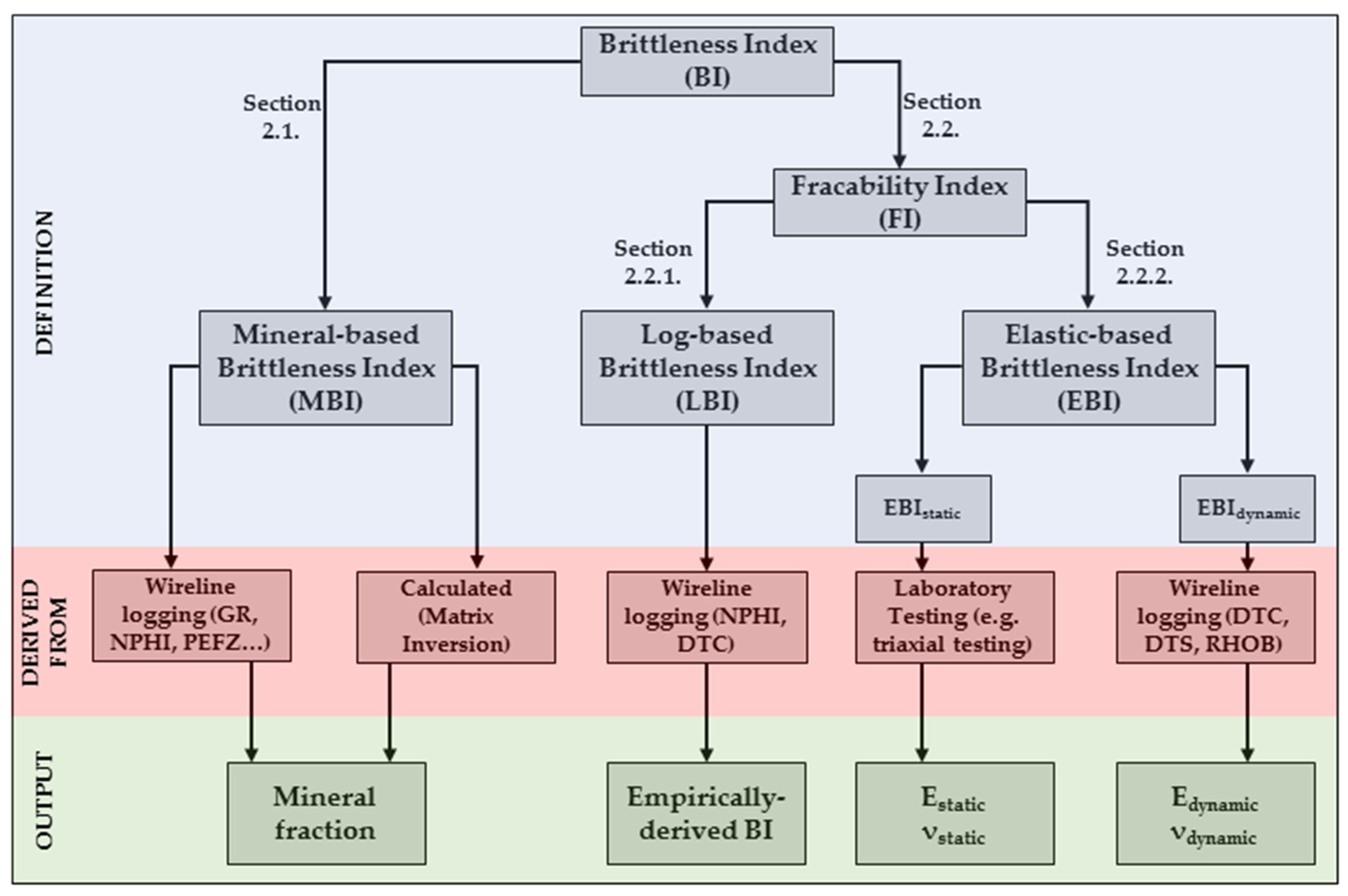
Figure 2.
Ternary diagram showing the average mineral content for the following formations: Niobrara Formation [40], Eagle Ford Shale [27], Marcellus Formation [41], middle Bakken Formation [42], Woodford/ Chattanooga Shale [25], Wolfcamp Formation [20,21], and Barnett Formation [12].
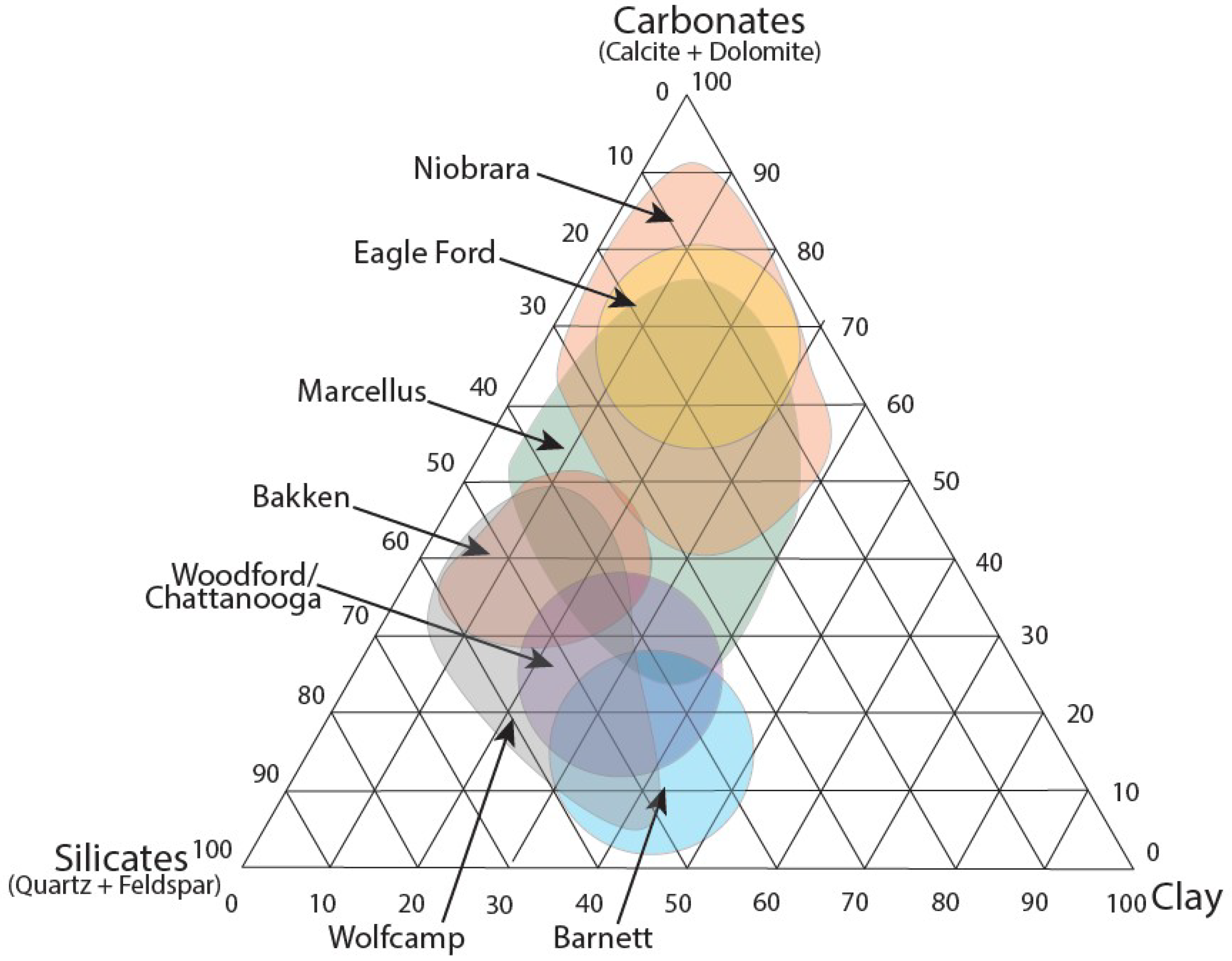
Figure 3.
Comparison between the MBI derived using the Glorioso and Rattia [16] correlation and the mineral weight fraction applied on the Marcellus Formation. (a) Comparison with a quartz weight fraction. (b) Comparison with a carbonate (calcite and dolomite) weight fraction.
Figure 3.
Comparison between the MBI derived using the Glorioso and Rattia [16] correlation and the mineral weight fraction applied on the Marcellus Formation. (a) Comparison with a quartz weight fraction. (b) Comparison with a carbonate (calcite and dolomite) weight fraction.

Figure 4.
Correlation between the clay (illite) content and the MBI based on the correlation from Glorioso and Rattia [16] applied on the Marcellus Formation. The data are derived from the Marcellus Formation in West Virginia.
Figure 4.
Correlation between the clay (illite) content and the MBI based on the correlation from Glorioso and Rattia [16] applied on the Marcellus Formation. The data are derived from the Marcellus Formation in West Virginia.

Figure 5.
BI correlations from the Marcellus Formation applied over depth. Black colors show LBI correlations and red colors show MBI correlations.
Figure 5.
BI correlations from the Marcellus Formation applied over depth. Black colors show LBI correlations and red colors show MBI correlations.
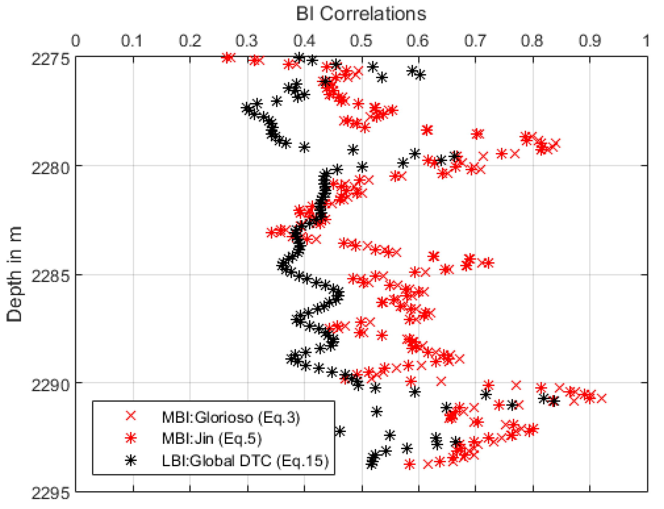
Figure 6.
BI correlations from the middle Bakken formation applied over depth. Black colors show LBI correlations, green colors modified MBI correlations (Table 4), and blue colors indicate EBI correlations. The interval from 3087.5 to 3102 m depth shows the middle Bakken formation. It shows a clear trend to the upper and lower Bakken since the clay content in these formations is significantly higher [42].
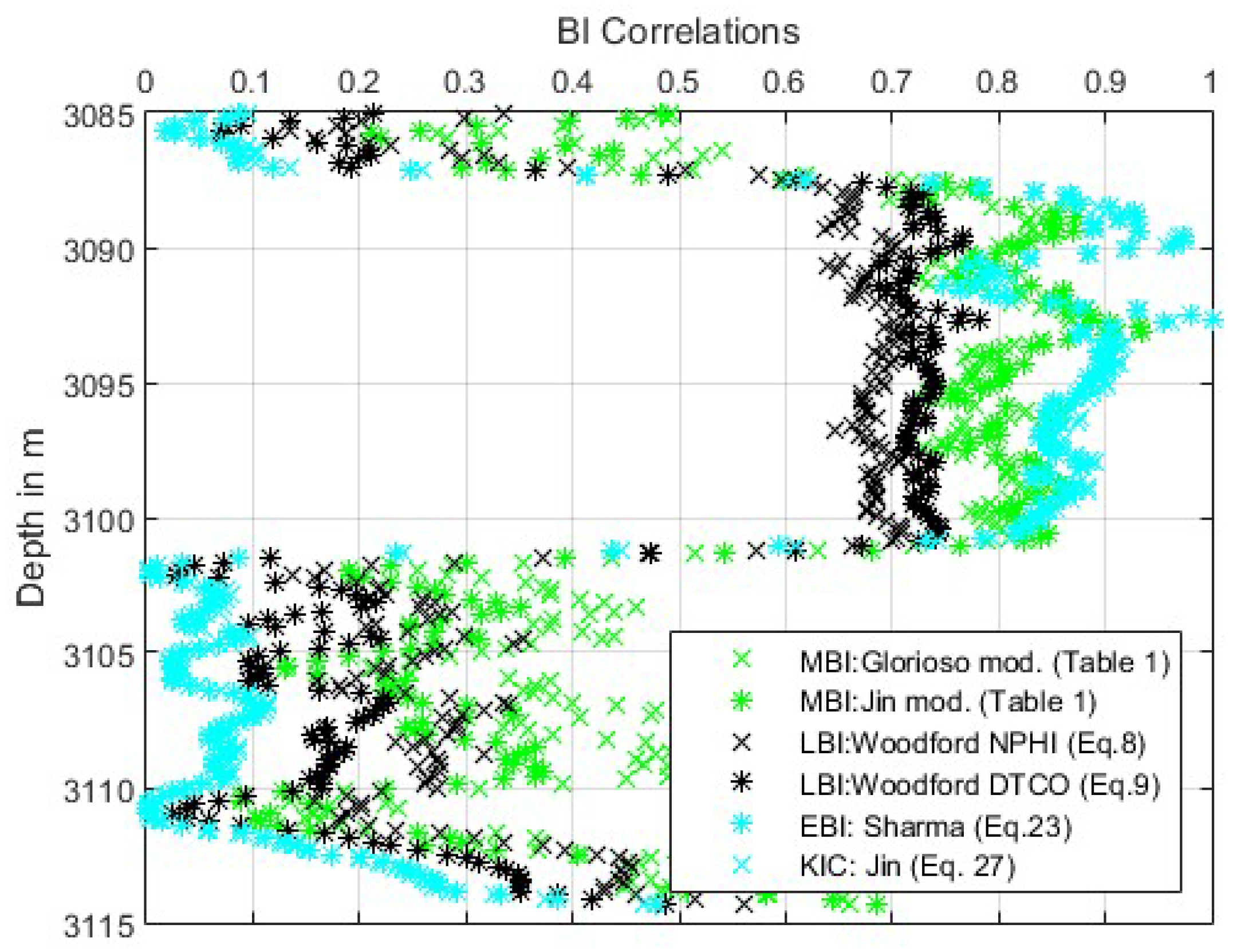
Figure 7.
BI correlations from the Niobrara Formation applied over depth. Black colors show LBI correlations, red colors show MBI correlations, and blue colors indicate EBI correlations. The EBI is overall significantly lower than LBI and MBI correlations.
Figure 7.
BI correlations from the Niobrara Formation applied over depth. Black colors show LBI correlations, red colors show MBI correlations, and blue colors indicate EBI correlations. The EBI is overall significantly lower than LBI and MBI correlations.
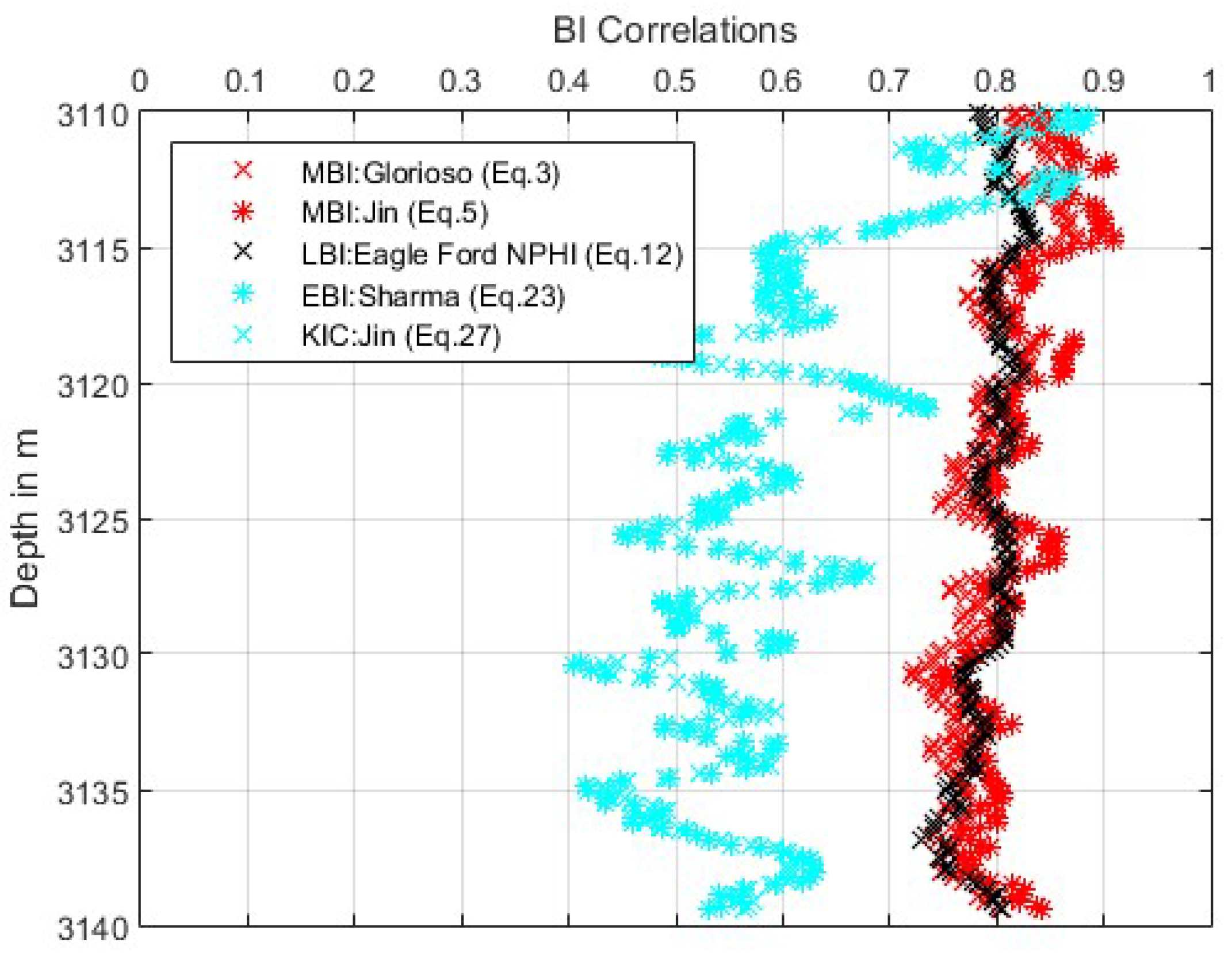
Figure 8.
BI correlations from the Chattanooga Shale applied over depth. Black colors show LBI correlations, red colors show MBI correlations, and blue colors indicate EBI correlations. The sharp change at 1506 m depth is due to a change in lithology from a silt dominated lithology with lower BI values to a dolomite dominated lithology with significantly higher values for BI.

Table 1.
Summary of MBI correlations based on the mineral composition.
| Correlation for MBI | Formation | Age | Lithology | Φ (%) | TOC (%) | Reference |
|---|---|---|---|---|---|---|
| Barnett | Carb. | Shale bounded by limestone | 6 | 1–3 | Jarvie et al. [12] | |
| Barnett | Carb. | Shale bounded by limestone | 6 | 1–3 | Wang and Gale [8] | |
| Neuquén Basin, Argentina | Jur. | Mudstones | 8 | 2.5–3.5 | Glorioso and Rattia [16] | |
| Haynes-ville | Jur. | Calcite to silica-rich shale | 8 | 3–6 | Buller et al. [17] | |
| Barnett | Carb. | Shale bounded by limestone | 6 | 1–3 | Jin et al. [19] | |
| Wolf-camp | Carb. - Perm. | Shale, minor limestone | 10 | 2.3 | Alzahabi et al. [20] | |
| Shales in Europe and Barnett | Camb. – Jur. | Shale bounded by limestone | 0.6–11 | 15 | Rybacki et al. [22] |
Table 2.
Summary LBI correlations based on compressional wave travel time (DTC) and neutron porosity (NPHI).
Table 2.
Summary LBI correlations based on compressional wave travel time (DTC) and neutron porosity (NPHI).
| Correlation for LBI | Formation | Age | Lithology | Φ (%) | TOC (%) | Reference |
|---|---|---|---|---|---|---|
| Woodford | Dev. | Shale bounded by limestone | 0.5–3 | 5.01–14.81 | Jin et al. [13] | |
| Barnett | Carb. | Shale bounded by limestone | 6 | 1–3 | Jin et al. [13] | |
| Eagle Ford | Creta. | Mudstones | 2–9 | 2.1–6.86 | Jin et al. [13] | |
| Global Correlation | - | - | - | - | Jin et al. [13] |
Table 3.
Summary of EBI correlations based on elastic properties.
| Correlation | Formation | Age | Lithology | Φ (%) | TOC (%) | Reference |
|---|---|---|---|---|---|---|
| Barnett | Carb. | Shale bounded by limestone | 6 | 1–3 | Rickmann et al. [28] | |
| Western Canadian Basin | Jur. | Shale and Sandstone | 5–10 | - | Sharma and Chopra [33] | |
| Liahoe, China | Paleogene | Shale | 2.39 | Sun et al. [35] | ||
| - | - | Shale and Sandstone | <10 | - | Chen et al. [36] | |
| Woodford | Dev. | Shale bounded by limestone | 0.5–3 | 5.01–14.81 | Jin et al. [19] | |
| Barnett | Carb. | Shale bounded by limestone | 6 | 1–3 | Jin et al. [19] | |
| Barnett | Carb. | Shale, bounded by limestone | 6 | 1–3 | Jin et al. [19] | |
| Barnett | Carb. | Shale bounded by limestone | 6 | 1–3 | Jin et al. [19] | |
| Barnett | Carb. | Shale bounded by limestone | 6 | 1–3 | Jin et al. [19] |
Table 4.
Modified MBI correlations showing the total porosity (PHIT) as an additional parameter in the denominator, which decreases the brittleness.
© 2019 by the authors. Licensee MDPI, Basel, Switzerland. This article is an open access article distributed under the terms and conditions of the Creative Commons Attribution (CC BY) license (http://creativecommons.org/licenses/by/4.0/).
Share and Cite
MDPI and ACS Style
Mews, K.S.; Alhubail, M.M.; Barati, R.G. A Review of Brittleness Index Correlations for Unconventional Tight and Ultra-Tight Reservoirs. Geosciences 2019, 9, 319. https://doi.org/10.3390/geosciences9070319
AMA Style
Mews KS, Alhubail MM, Barati RG. A Review of Brittleness Index Correlations for Unconventional Tight and Ultra-Tight Reservoirs. Geosciences. 2019; 9(7):319. https://doi.org/10.3390/geosciences9070319
Chicago/Turabian StyleMews, Kim S., Mustafa M. Alhubail, and Reza Gh. Barati. 2019. "A Review of Brittleness Index Correlations for Unconventional Tight and Ultra-Tight Reservoirs" Geosciences 9, no. 7: 319. https://doi.org/10.3390/geosciences9070319
Note that from the first issue of 2016, this journal uses article numbers instead of page numbers. See further details here.