An Evaluation of Catchment Transit Time Model Parameters: A Comparative Study between Two Stable Isotopes of Water

Abstract

Using δ¹⁸O and δ²H in mean transit time (MTT) modeling can ensure the verifiability of results across catchments. The main objectives of this study were to (i) evaluate the δ¹⁸O- and δ²H-based behavioral transit time distributions and (ii) assess if δ¹⁸O and δ²H-based MTTs can lead to similar conclusions about catchment hydrologic functioning. A volume weighted δ¹⁸O (or δ²H) time series of sampled precipitation was used as an input variable in a 50,000 Monte Carlo (MC) time-based convolution modeling process. An observed streamflow δ¹⁸O (or δ²H) time series was used to calibrate the model to obtain the simulated time series of δ¹⁸O (or δ²H) of the streamflow within a nested system of eight Prairie catchments in Canada. The model efficiency was assessed via a generalized likelihood uncertainty estimation by setting a minimum Nash–Sutcliffe Efficiency threshold of 0.3 for behavioral parameter sets. Results show that the percentage of behavioral parameter sets across both tracers were lower than 50 at the majority of the studied outlets; a phenomenon hypothesized to have resulted from the number of MC runs. Tracer-based verifiability of results could be achieved within five of the eight studied outlets during the model process. The flow process in those five outlets were mainly of a shallow subsurface flow as opposed to the other three outlets, which experienced other additional flow dynamics. The potential impacts of this study on the integrated use of δ¹⁸O and δ²H in catchment water storage and release dynamics must be further investigated in multiple catchments within various hydro-physiographic settings across the world.

1. Introduction

Mean transit time (MTT) has been globally used as an effective metric for describing the water storage and release mechanisms of catchments. The MTT is defined as the average time water spends travelling from an input point (such as the catchment surface) to an output point (which could be a stream outlet or a well) [1]. MTT has important applicability in evaluating the streamflow generation processes [2,3,4] and the characterization of controls on weathering rates [5,6] and identifying the catchment response to climate change [7,8,9].

There are various approaches to evaluating catchment MTT. Popular methods include: Convolution integral modeling, either in the time domain [4] or in the frequency domain (also called the spectral method) [10]; sine-wave modeling, which relies on the annual sinusoidal cycle of precipitation and streamflow isotopic composition (e.g., [11]); and the most recent methods that rely on StorAge Selection (SAS) functions (e.g., [12,13]). Even though SAS functions are emerging, they are not mainstream yet, mainly due to difficulties in estimating total catchment storage as part of the model input requirements [13]. Thus, the traditional convolution integral modeling in the time domain, also called the time-base convolution (TBC), still serves as a popular and effective MTT modeling approach, especially with the recent introduction of stable water isotopes as tracers in catchment MTT studies.

Both chemical and isotopic tracers have, over the years, been applied in studies involving catchment water storage and release dynamics. Examples of applicable studies include stream water partitioning into pre-event (water that existed in streams before the onset of current precipitation events) and event (water brought about by the current precipitation event) fractions. Other examples involve catchment MTT studies, ecohydrological functioning, and many more [1,14,15]. Earlier studies relied heavily on the use of chemical tracers, such as chloride, silica, and calcium [10,16,17], with the assumption that those tracers behaved in a conservative manner. The chemical characteristics of conservative tracers, as they move through watersheds, are supposed to remain unaffected by water transport processes, but that is rarely the case with ions. Indeed, most chemicals either undergo reactions with other salts, change state by precipitation, and thus do not leave the watershed at all, or are taken up by biota [18,19]. Notably, chloride is known to be chemically inert, but it is still used up by biota to some degree. In contrast, the use of stable water isotopes (δ¹⁸O and δ²H) as conservative tracers has proven to be an effective tool in catchment storage and release dynamics studies [20,21,22]. Catchment MTTs have been evaluated with chloride (e.g., [10]), but the use of stable isotopes of water (e.g., δ¹⁸O and δ²H) is dominant in many recent models. Majority of MTT studies relying on the TBC method—still the most traditionally used method—have applied only a δ¹⁸O tracer, but some have also used δ²H data (e.g., [23]). A few others have used both δ¹⁸O and δ²H data in their studies (e.g., [24,25]). While collinearity between δ¹⁸O and δ²H behavior may be assumed to exist, some studies have argued that modeling performed using both tracers can help in inferring the acceptability of results in light of fractionation processes (e.g., [4]). With fractionation affecting δ²H more than it does affect δ¹⁸O, the question then arises as to whether the use of both tracers—even if they provide different absolute values of MTTs—can help scientist draw similar conclusions about a catchment. Despite the time spent in repeating yet another lengthy model run for δ²H data, after the completion of the δ¹⁸O run, results from each data can reveal interesting catchment characteristics. It can be potentially rewarding to use both δ¹⁸O and δ²H in the hydrological modeling process to evaluate MTT.

The performance of every hydrological model is reported via comparisons between simulated and observed variables. In most cases, this comparison is made between the simulated and observed streamflow at the catchment outlet. How close simulated variables are to the observed is measured by a chosen model efficiency criterion. In catchment MTT studies, the two most popular criteria are the Nash–Sutcliffe efficiency (NSE) and the coefficient of determination (R²). We undertook a review and deduced that these two model efficiency criteria have been adopted in 92% of 68 published MTT papers within the past 10 years. The papers that employed the NSE criterion mostly set NSE = 0.2 as a threshold for extracting behavioral parameters. Behavioral parameters are the optimal model parameters (assumed to have efficient goodness of fits of observed and simulated variables) that are isolated and evaluated for the actual MTT determination. Studies that have relied on δ²H data in MTT hydrological models are few and far between. The question then remains unanswered as to whether δ²H data can give similar information about a system as δ¹⁸O data does. In this current study, we used multiple seasons of precipitation and streamflow δ¹⁸O and δ²H time series data to determine the catchment MTT. This was undertaken within a system of eight nested catchments in Manitoba, Canada. The TBC modeling process was employed and model performance efficiency was evaluated via the NSE [26]. The objectives of this study were three-fold:

• To evaluate the distribution of δ¹⁸O- and δ²H-based behavioral parameters from which the MTT was extracted.
• To determine how early in the model time-step δ¹⁸O- and δ²H-based behavioral solutions are achieved.
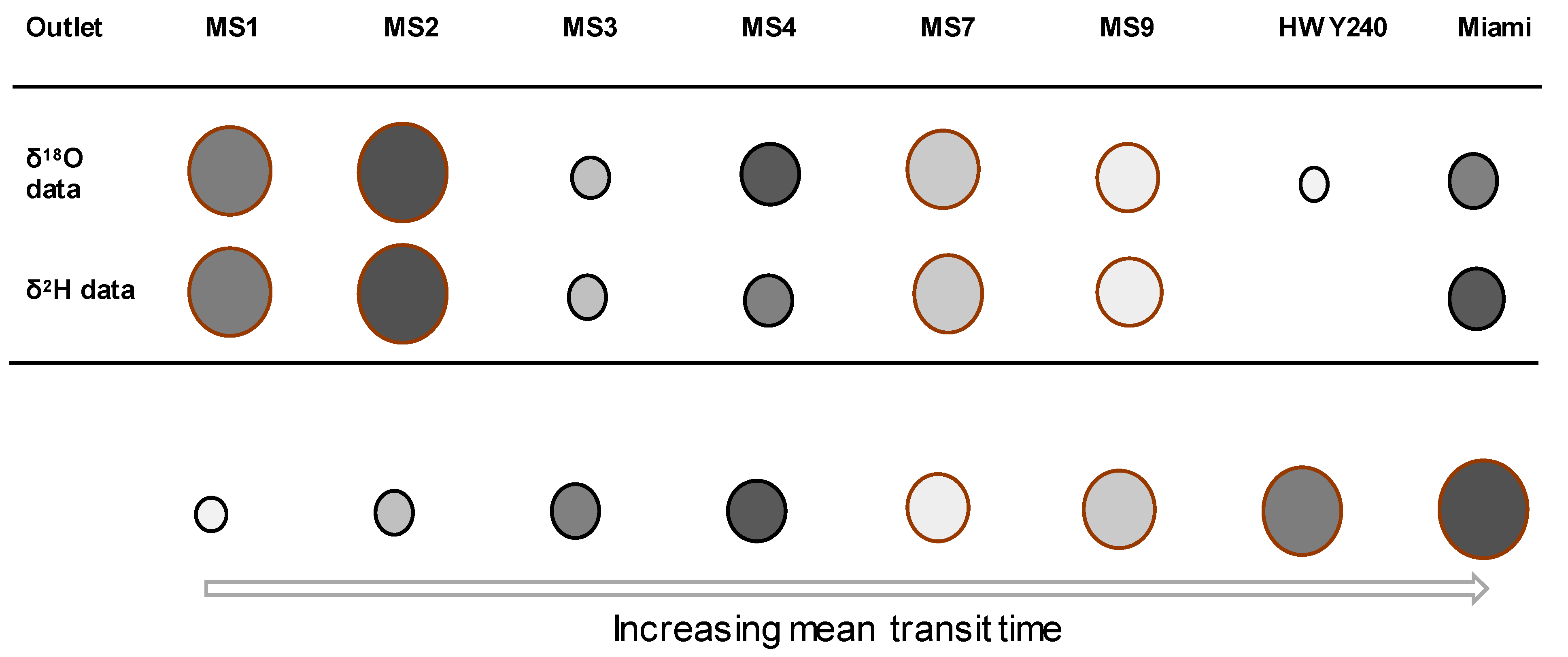
• To assess the agreement (or lack thereof) of the absolute MTT values as retrieved from the δ¹⁸O and δ²H model kernels and to infer if they lead to similar conclusions about the nested catchment system.

Achieving the objectives will potentially help inform watershed scientists on the implications of applying the dual water isotopes (δ¹⁸O and δ²H) in catchment water storage and release dynamics studies in light of the influence of evaporative processes on the study results. This will help in advancing studies on ways to improve result acceptability in TBC MTT modeling.

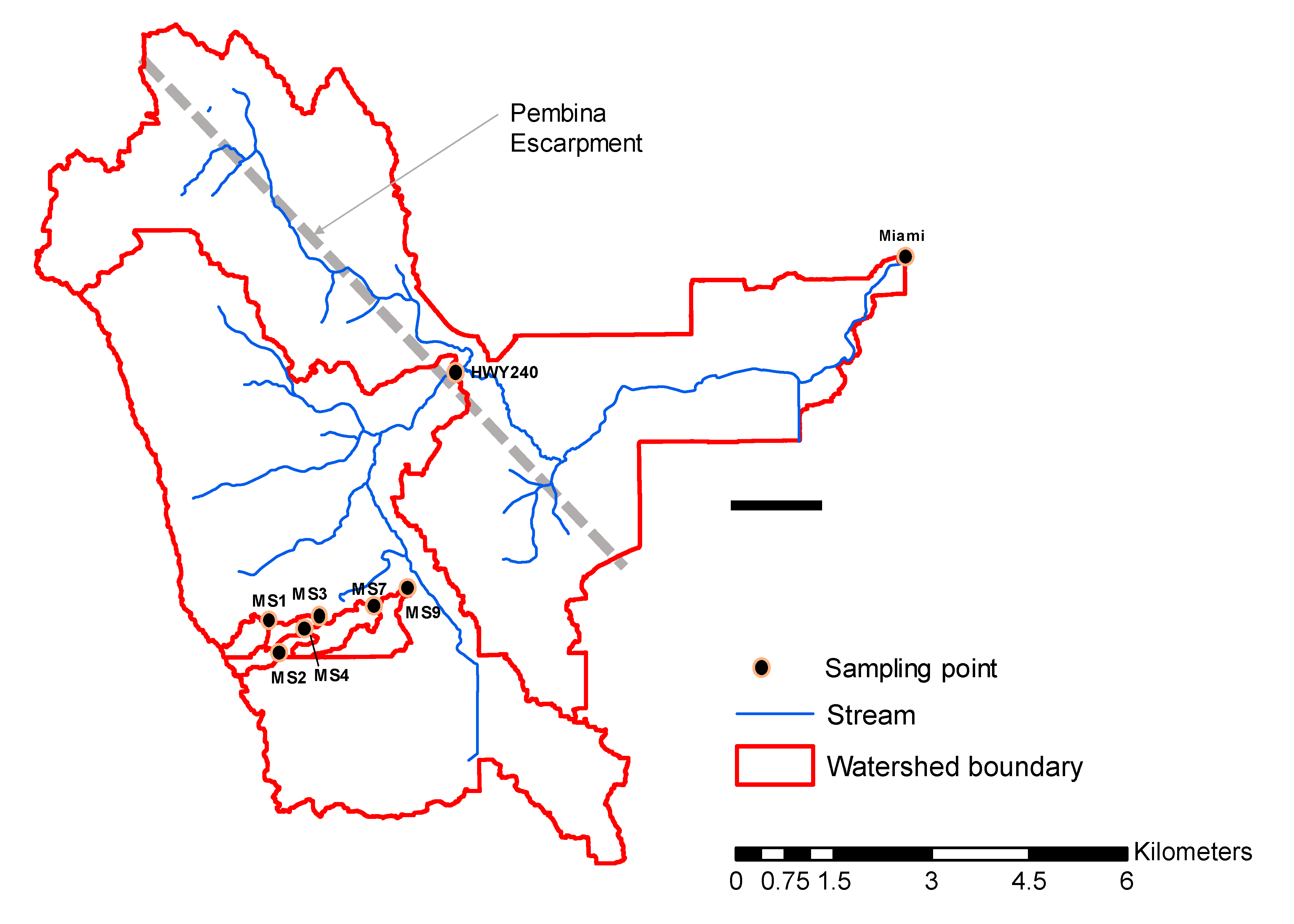
2. Materials and Methods

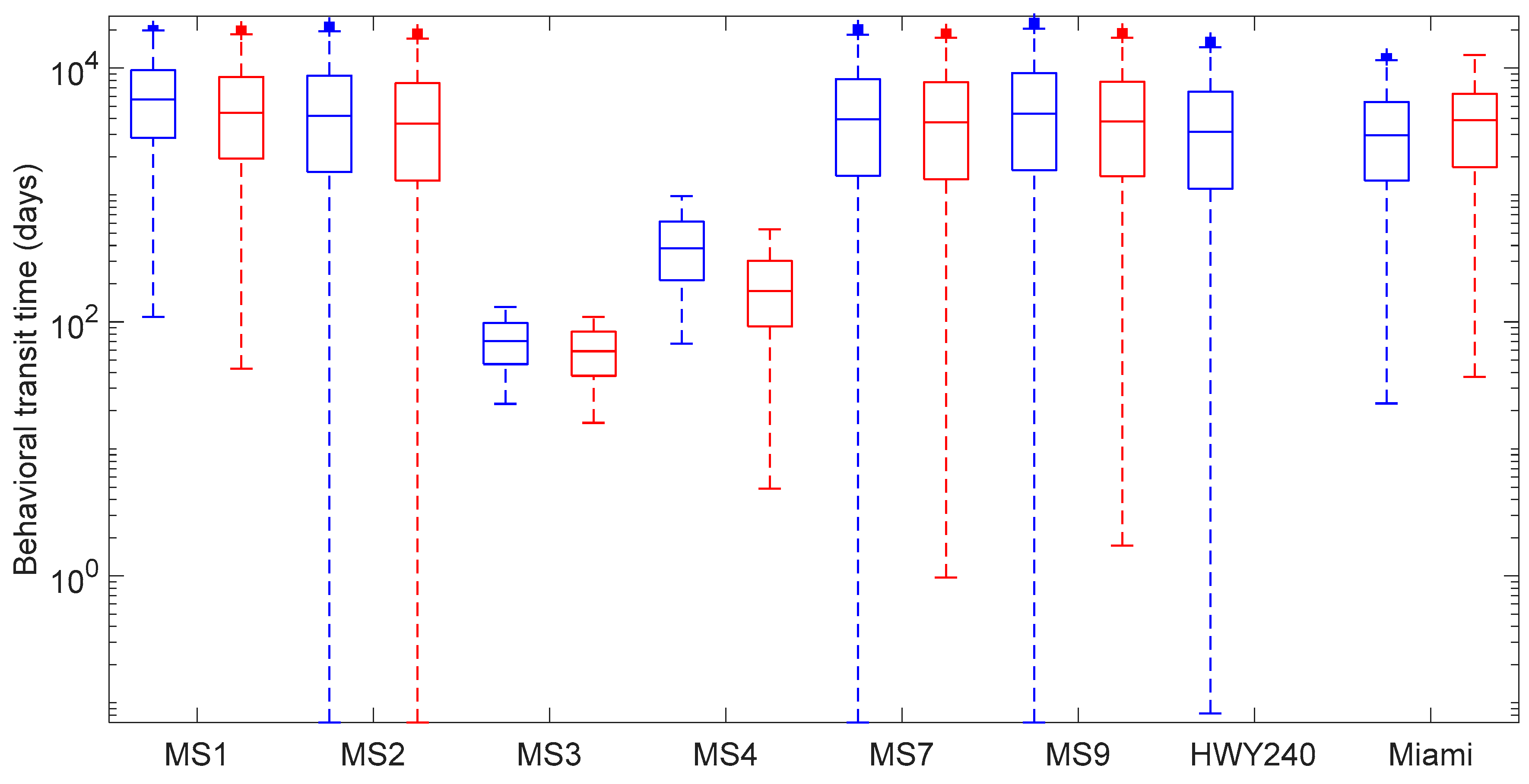
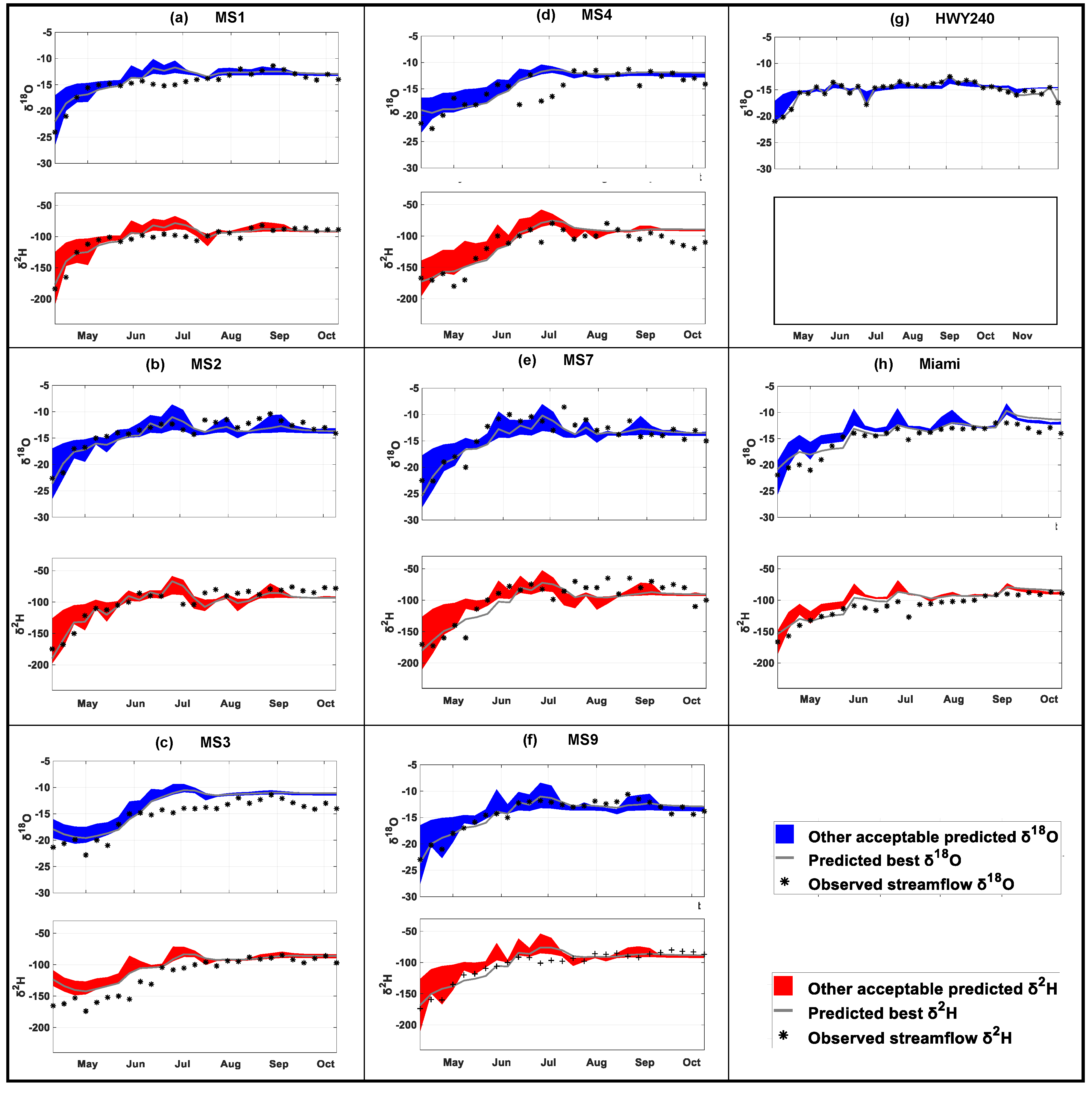
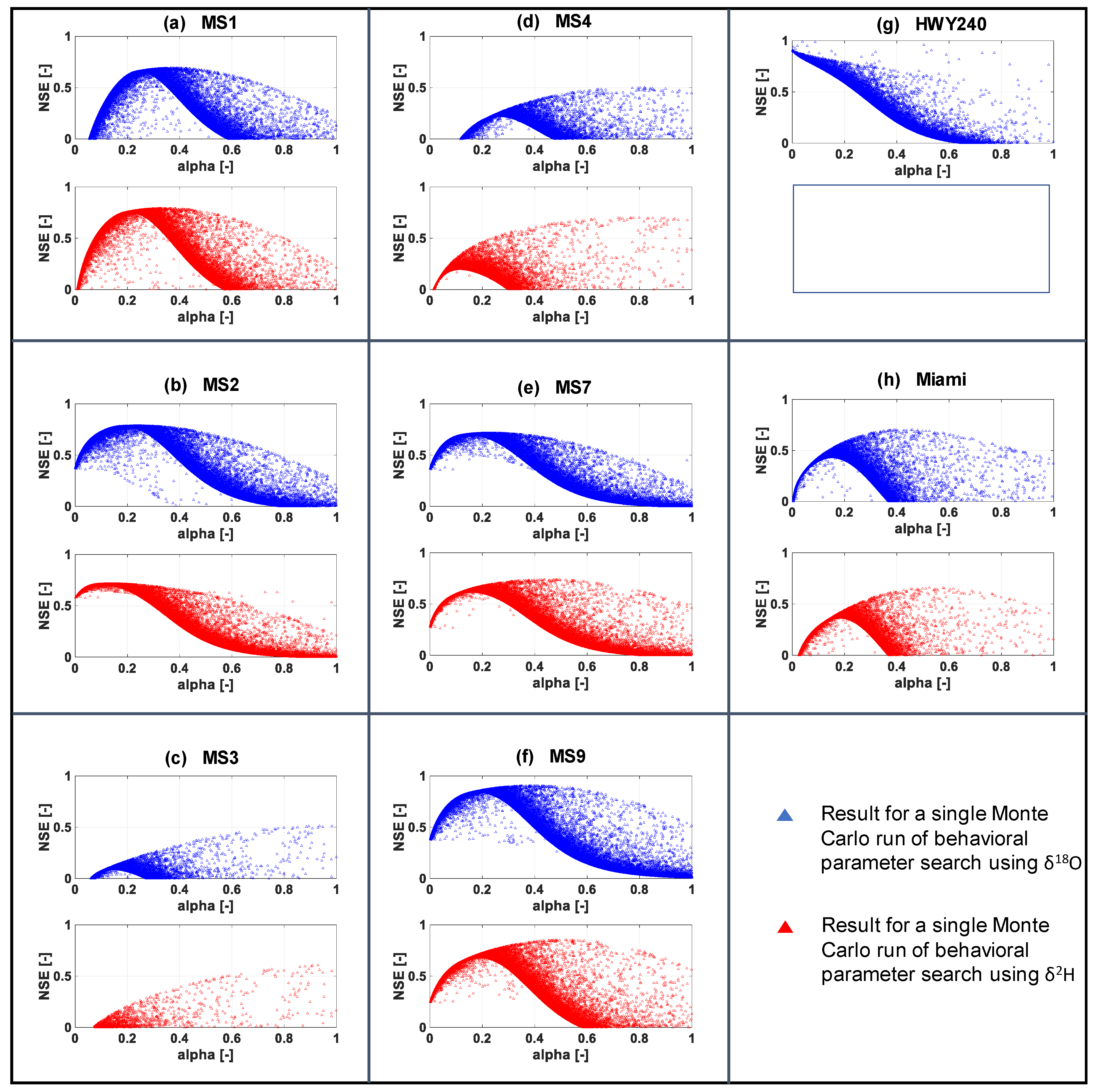
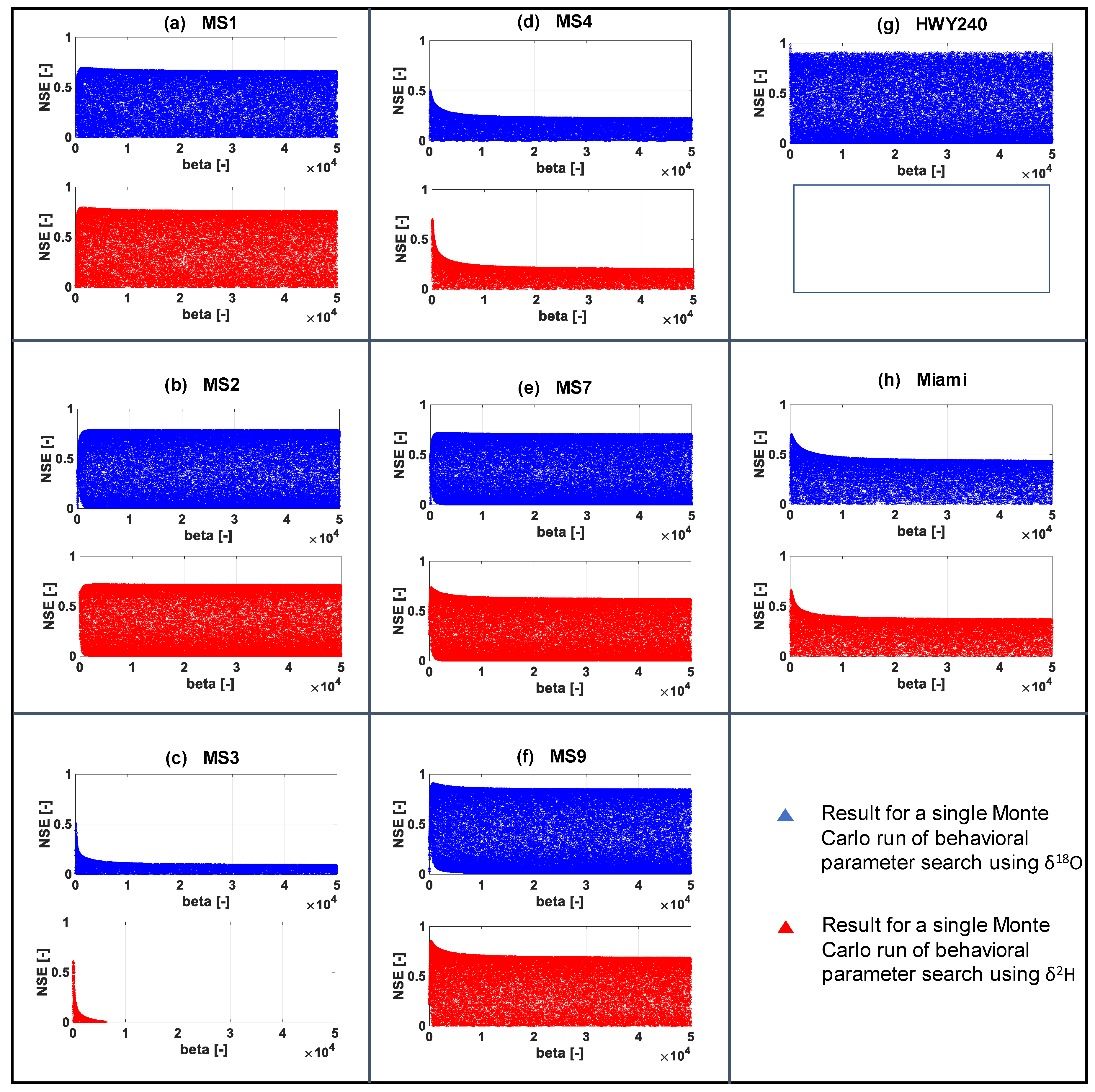
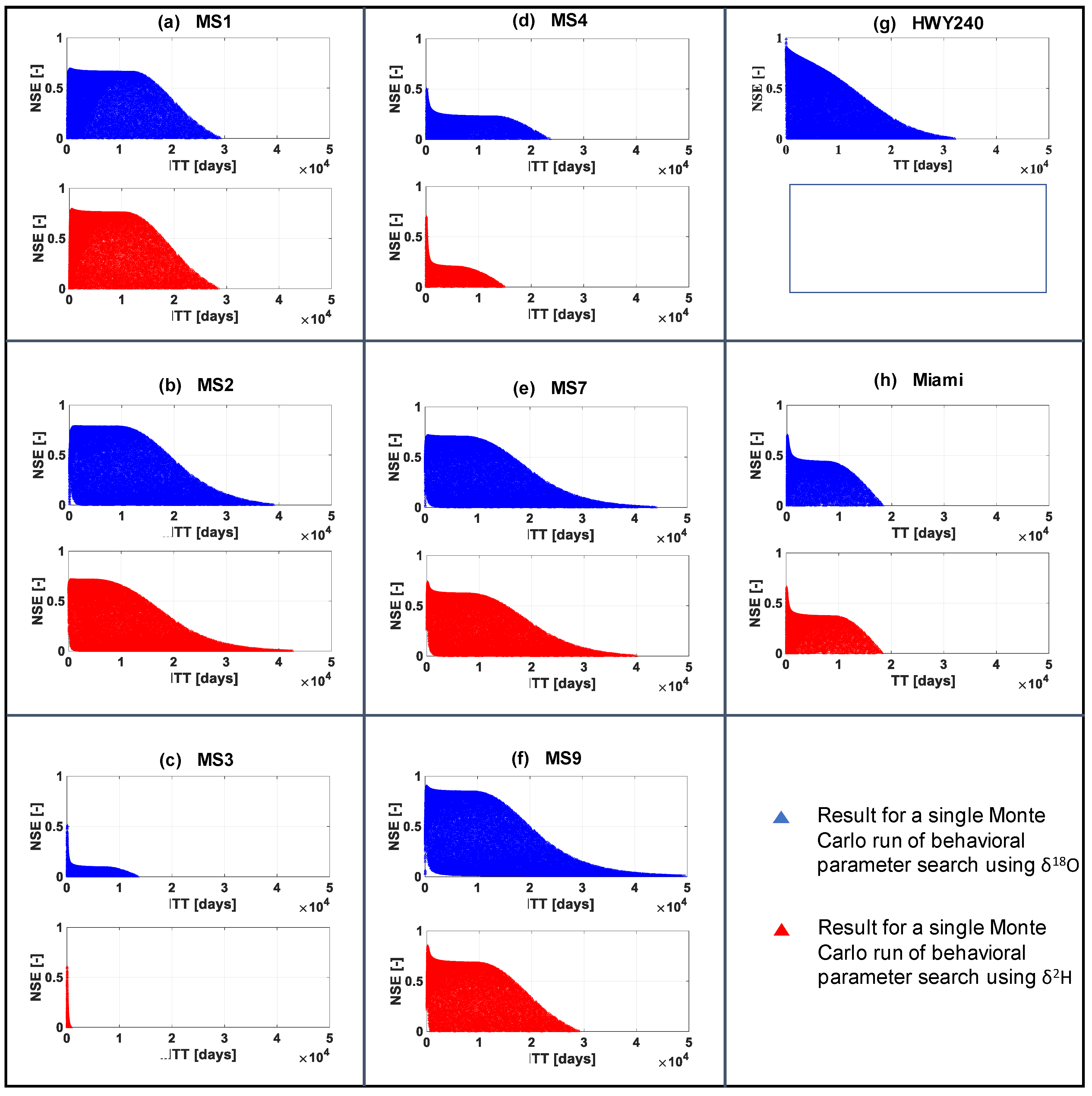
The focus of this study was on a nested system of a 74.4 km² catchment comprising of eight outlets. The outlets are named in order of flow regime from upstream to downstream as MS1, MS2, MS3, MS4, MS7, MS9, HWY240, and Miami (with 0.28, 0.19, 0.48, 0.31, 1.27, 1.88, 34.6, and 74.4 km² as corresponding areas, respectively); MS1 and Miami forming the headwater and final exit, respectively, of the whole catchment system. This nested system of catchments, called the South Tobacco Creek Watershed (STCW), was located in south central Manitoba, Canada (Figure 1). The STCW was generally composed of a shale bedrock overlain by moderate to strong calcareous glacial till and clay-loam soils [27]. The HWY240 outlet sat on the edge of a NW-SE trending escarpment, also called the Pembina Escarpment. The MS4 and MS7 outlets had small retention ponds located immediately upstream for stormwater control purposes; the pond behind MS7 had the tendency to overflow during snowmelt and extreme storm events. Total annual precipitation was 529.5 mm (including 30% of snowfall), while the mean daily air temperature was 2.9 °C [28]. Long term (1991–2014) values of mean total annual precipitation was 512.3 mm, while that of mean daily air temperature was 2.86 °C [28]. Precipitation (including snowmelt captured by snow lysimeters) and stream water samples were collected from the eight outlets across multiple seasons (spring, summer, and fall) of 2014, at a frequency of at least once every week. The sampling period began during the freshet (in March) and ended just at the start of the snowfall in October. Concurrently, precipitation amounts were obtained from the nearby weather survey of the Canada station. All the samples were stored in 10 mL glass vials, sealed with parafilm, and kept at 4 °C until analysis. They were then tested for δ¹⁸O and δ²H using a Picarro^TM Liquid Water Isotope Analyzer (LWIA, model L2130-i) based on cavity ring-down spectroscopy (CRDS) technology. Delta (δ) values were recorded in permil (‰) deviations from the Vienna standard mean ocean water (VSMOW) [29], with a precision of 0.025 ‰ and 0.1 ‰ for δ¹⁸O and δ²H, respectively. Time series of δ¹⁸O (or δ²H) of precipitation and streamflow were obtained. We then assumed the transit time distribution ((TTD) g(τ))—the kernel from which the mean transit time (MTT) is extracted from—of the nested catchment system to belong to a family of gamma distributions (Equation (1)) for which the ((MTT (τ)) is equivalent to αβ (Equation (2)): The assumption of a choice of a gamma transfer function was appropriate based on the general geology of the catchment and was confirmed by comparisons of goodness-of-fit values during the initial model optimization process of “small model runs”, where other transfer functions were also tested.

$$g\left(\tau \right)=\frac{{\tau }^{\alpha -1}}{{\beta }^{\alpha }\mathsf{\Gamma }\left(\alpha \right)}ex{p}^{-\tau /\beta }$$

(1)

$$\tau =\alpha \beta$$

(2)

where α and β are the shape and scale factors of the gamma distributions, respectively.

Convolution integral modeling was performed in the time domain using the δ¹⁸O time series data of precipitation and streamflow, which was then repeated for the δ²H data. The two-parameter gamma distribution model, chosen for the catchment system, was selected as a stationary TTD (noted as g(t – τ)) and convolved with the amount-weighted δ¹⁸O (or δ²H) isotopic timeseries of precipitation (δ_in(τ)) to predict the δ¹⁸O (or δ²H) isotopic timeseries in the streamflow (δ_out(t)) [4,30] via Equation (3):

$${\delta }_{out}\left(t\right)= \underset{-\infty }{\overset{t}{{\displaystyle \int }}}{\delta }_{in}\left(\tau \right)g\left(t-\tau \right)d\tau$$

(3)

For each of the eight sub-catchments, the input data record was artificially filled or extended by a sine-wave approximation technique [31,32]. A 30-year warm-up period was used to actuate the model; the isotopic time series data was looped 30 times backward—a process referred to as a “loop scenario” (e.g., [33])—to achieve the warm-up condition, at the end of which the calibration process began. The search for behavioral model parameters was conducted by means of 50,000 Monte Carlo (MC) simulations in MATLABR2017b. A generalized likelihood uncertainty error (GLUE) [34] analysis was performed by setting a minimum Nash–Sutcliffe ffficiency (NSE) threshold of 0.3 for behavioral parameter sets. The MTT was estimated by multiplying the α and β parameters associated with the MC simulation that yielded the highest NSE.

To help evaluate the first research objective, all behavioral parameter sets of α and β (i.e., the α and β values of all the MC simulations (out of the 50,000) that resulted in NSE scores of 0.3 and above) were retrieved from the δ¹⁸O- and δ²H-based models. Boxplots were then used to assess the distribution of transit times (TTs) within each tracer category. The percentage of simulations (out of the 50,000) that resulted in behavioral parameter sets within the δ¹⁸O and δ²H tracer categories was evaluated. The time-step of the MC simulation, at which the behavioral parameter sets corresponding to the highest NSE occurred, was noted for both δ¹⁸O and δ²H tracers and used to evaluate the second research objective. The third and final research objective was evaluated by multiplying the α and β parameter sets that corresponded with the MC simulation associated with the highest NSE. This was performed for both tracers and for all eight sub-catchments. Standard errors (±1σ) around the MTT were calculated from the behavioral TTs that emerged from the 95th percentile of NSEs. To ascertain if there were any significant differences (or lack thereof) between δ¹⁸O- and δ²H-based MTTs, a Spearman’s rank correlation analysis was performed at the 95% significance level. The catchments were then assessed in the context of increasing order of MTTs according to both tracers.

3. Results

The maxima of the transit time distribution (TTD) at the outlets appear to be higher for the δ¹⁸O category than the δ²H, the only exception being at the Miami outlet. In contrast, the minima TTDs appear to be generally lower for the δ²H class than for δ¹⁸O (Figure 2). The maximum TT was about 10,000 days for the δ¹⁸O class and about 9900 days for the δ²H class. A spearman’s rank correlation analysis of the maximum TT across the eight sites showed no significance at the 95% level between the δ¹⁸O- and δ²H-based TTs (Rho = 0.61; p-value = 0.38). The maximum TT values across the studied outlets appear to occur at outlets MS1 and MS9 for each tracer class (Figure 2). The minimum TT was 80 days and 70 days, respectively, for the δ¹⁸O and δ²H class, both occurring at site MS3. The median TTs were higher within the δ¹⁸O class at all the outlets except Miami (Figure 2). Within the δ¹⁸O class, the highest median TT was about 6000 days and occurred at outlet MS1. A total of 4000 days was the highest median TT within the δ²H category, and it also occurred at outlet MS1 (Figure 2). There were no marked differences in the ranges of TT values between the δ¹⁸O and δ²H classes across the sites, since the tracer specific boxes appear similar in size. All TT outliers appear to be on the upper end of the distribution in each tracer category, with values above 11,000 days (Figure 2). The only outlets without TT outlier values were MS3, MS4, and the δ²H-based tracer class for Miami (Figure 2). There was generally a lower percentage of behavioral TT (out of the 50,000 MC runs) within each δ¹⁸O and δ²H class across all the eight outlets; with values at MS3 and MS4, for instance, being less than 2% (

Table 1. δ¹⁸O- and δ²H-based behavioral solutions across the eight study outlets. Behavioral parameters were selected from 50,000 Monte Carlo simulations in MATLABR2017b (The MathWorks, Natick, MA, USA). [ ] show ±1σ around the mean. NB: No behavioral solutions were found (i.e., all Nash–Sutcliffe efficiencies (NSEs) were less than 0.3).

Variable	Tracer	MS1	MS2	MS3	MS4	MS7	MS9	HWY240	Miami
Total number of behavioral outcomes	δ18O-based	17,467	24,796	99	515	23,267	26,199	18,515	12,210
	δ2H-based	20,618	21,696	96	755	22,221	21,992	0	8497
Percentage of behavioral outcomes	δ18O-based	35	50	<1	1	47	52	37	24
	δ2H-based	41	43	<1	2	44	44	0	17
Best NSE score (-)	δ18O-based	0.69	0.79	0.51	0.50	0.72	0.90	0.99	0.70
	δ2H-based	0.79	0.71	0.61	0.70	0.74	0.85	NB	0.66
Alpha value corresponding to the best NSE score (-)	δ18O-based	0.39	0.23	0.93	0.82	0.24	0.39	0.04	0.46
	δ2H-based	0.32	0.14	0.93	0.78	0.44	0.52	NB	0.52
Count of Monte Carlo run where alpha best was observed	δ18O-based	43,310	19,915	47,134	43,865	30,875	23,107	33,308	40,627
	δ2H-based	30,307	48,520	47,220	49,490	17,550	15,369	NB	37,956
Beta value corresponding to the best NSE score (-)	δ18O-based	1409	4747	66	140	2163	745	2	207
	δ2H-based	1477	3701	50	75	363	300	NB	182
Time-step of Monte Carlo run where beta best was observed	δ18O-based	43,310	19,915	47,134	43,865	30,875	23,107	33,308	40,627
	δ2H-based	30,307	48,520	47,220	49,490	17,550	15,369	NB	37,956
Mean transit time (days)	δ18O-based	549 [± 63]	1155 [± 18]	62 [± 3]	115 [± 3]	509 [± 34]	287 [± 10]	<1 [± 0.1]	95 [± 7]
	δ2H-based	482 [± 53]	507 [± 33]	47 [± 1]	58 [± 1]	158 [± 2]	157 [± 15]	NB	95 [± 4]

). There was no behavioral TT parameter at outlet HWY240 within the δ²H class (Figure 2 and Figure 3; Table 1). In general, across all the outlets, there was a higher number of behavioral parameters within the TTD of the δ¹⁸O tracer than there was for δ²H (Table 1). The GLUE bound appears to show some seasonality in the prediction of the δ output variable; the uncertainty band is bigger during the freshet and smaller as the season progresses into summer and fall (Figure 3).

The α (shape factor) values corresponding to the best NSE score at the outlets ranged from 0.04 to 0.93 for the δ¹⁸O-based tracer and 0.14 to 0.93 for the δ²H-based tracer (Figure 4; Table 1). The β (scale factor) counterparts were 2 to 4747 for the δ¹⁸O-based tracer and 50 to 3701 for the δ²H-based counterpart (Figure 5; Table 1). The highest α, corresponding to the highest NSE, occurred at outlet MS3 in both tracer classes whiles the lowest occurred at outlet HWY240 within the δ²H class. Within the δ¹⁸O class, the highest β, corresponding to the highest NSE, occurred at outlet MS2 while the lowest occurred at HWY240. The highest δ²H-based β also occurred at outlet MS2 while the lowest occurred at outlet MS3 (Table 1). The time-step for the convergence on the best α at all the eight outlets matches the time-step for converging on β (Table 1). In general, and within each tracer class, the simulation appears to be converging on the best behavioral α and β at later time-steps (beyond time-step 25,000) (Table 1). The absolute MTTs from the δ¹⁸O- and δ²H-based tracers were different except for the value at the Miami outlet (95 days for both tracer categories) (Figure 6h). In general, the MTT of the catchments in this study were less than 9 months (Table 1). However, tracer specific MTTs at the outlets were, different. A significance test at the 95% level did not show any association between δ¹⁸O- and δ²H-based MTT results (Rho = 0.56; p-value = 0.21). However, when the tracer specific MTTs were ranked in increasing order, five out of the eight outlets matched (Figure 7).

4. Discussion and Implications

A total of three major outcomes emerged from this study: (i) There were lower percentages (out of the 50,000 MC simulations) of behavioral parameters (parameters that passed the NSE > 0.3 threshold) at all the eight outlets for both the δ¹⁸O- and δ²H-based data; (ii) time-steps for the retrieval of the best behavioral shape and scale parameters associated with both tracers occurred at latter times of the simulation at the majority of outlets; and (iii) mean transit times associated with each tracer across the majority of outlets were less than nine months. Though δ¹⁸O-based MTTs did not match that of the δ²H category at the majority of outlets, there were general similarities in the outlet positions on the δ¹⁸O- and δ²H-based MTT ranks (Figure 7). Regarding outcome (i), the lower percentage of behavioral parameters makes it potentially easier for optimum behavioral parameter identifiability, but that also implies a lessening of the efficiency of model performance. Figure 4 and Figure 5 suggest model insensitivity in the majority of the parameter space for both tracers. This is especially evident for the scale parameter search (Figure 5), which assumes model sensitivity within few areas of the parameter space. This model behavior potentially reduces the efficiency of the search for behavioral solutions. For instance, some of the worse NSEs were observed at outlets MS3 and MS4 (0.51 and 0.61 for δ¹⁸O- and δ²H-based tracer at outlet MS3; and 0.5 and 0.7 for counterparts at outlet MS4) and these outlets correspond to the lowest percentage of behavioral parameters (less than 2% at each of those two outlets) (Table 1). Contrary to observations at outlets MS3 and MS4, results from outlets MS2, MS7, and MS9 show some of the best NSEs (Table 1). The outlets recording the best NSEs correspond to some of the highest percentages of behavioral parameters (Table 1) within both tracer categories across all eight outlets. Regarding Outcome (ii), behavioral solutions occurred at latter time-steps during the model run. This was observed within both tracer categories and across the majority of the studied outlets. This raises one key question: Does the model appear to be performing better as the simulation advances? If that is the case, then this has direct implications for model optimization in the form of the length of the warm-up period (which was 30 years in the current study) and the number of Monte Carlo simulations (which was 50,000 in this study). Given the average time it takes to complete these kinds of MATLAB-based MC MTT simulations (about two months for each tracer in the current study), it becomes imperative to consider other methods of model optimization which would constrain the parameter search space in order to make the model more efficient in the context of run times. Outcome (iii) reinforces the understanding that a lot of the water within the Canadian Prairie catchments is very young, i.e., less than three months old [11,35]. There is also the reaffirmation that absolute MTTs should not be interpreted as standalone values but must be confirmed with the convergence of results from other methods. This is particularly useful for the comparison of inter catchment storage functioning [25]. The lack of significant association between the two tracer-based MTTs highlights the potential effects of evaporative losses on, especially, the δ²H-based MTTs. Because the vapor pressure between ¹H/²H is higher than ¹⁶O/¹⁸O, residual evaporated water appears to be more enriched in δ²H compared to δ¹⁸O, since these two isotopes are unequally affected by kinetic fractionation [3,36]. This phenomenon may explain why no behavioral model parameters were recorded for the δ²H-based MTT at HWY240 (Figure 2, Figure 3, Figure 4, Figure 5 and Figure 6; Table 1). The fractionation dynamic is consistent with the prairies (a semi-arid terrain), where summer stream samples may be retrieved from stagnant (albeit slowly flowing) streams. Outcome (iii) further affirms the notion that the use of both δ¹⁸O and δ²H in modeling could help build confidence in result acceptability [4]: The ranking of the outlets using tracer specific MTTs leads to process implications as to why all eight outlets were not similarly ranked across the two tracers. A process interpretation, using isotope-based hydrograph separation techniques within the STCW [37], touts the five outlets that agreed in the context of δ¹⁸O and δ²H MTT ranks, as experiencing shallow subsurface flow (SSF) processes. The remaining three that failed to agree have other processes in play in addition to the SSF; MS4 experiences detention losses under the dam in between storm events; HWY240 receives water via deep percolation of passive stores of old water; and Miami receives Hortonian overland flow as well as groundwater upwelling during heavy storm events [35,37]. While a dossier of dominant flow processes across the Canadian prairies has been well documented in the study by [38], what is evident from this work, from the isotopic standpoint, is that during low flow conditions, sources of water in the stream may not necessarily be from deep groundwater, in view of the fact that the ages of the water are generally young (less than nine months). What this study rather appears to show is that SSF sources (made up of relatively young water) contribute greatly to streamflow at the majority of the studied outlets. One key exception was at the HWY240 outlet; the short MTT was at odds with the high old water fractions [37] and the relatively small fraction of young water (i.e., the fraction of stream water that is of age three months or less) [37]. However, further studies at HWY240, using hydrometric data [39], showed that runoff ratios were generally greater than 1 at HWY240, pointing to a potential piston flow mechanism akin to fast percolation of precipitation or meltwater through the fractured bedrock and the pushing out of old groundwater into the stream outlet in a manner consistent with the [40] version of celerity. The isotopic and hydrometric results validate the hypothesis that, at HWY240, the stream is fed by passive stores of groundwater during low flow conditions. The distribution of the α and β parameters in the NSE space across the sites (Figure 4 and Figure 5) appear consistent with relatively shorter arrival times for the δ²H-related TTs (Figure 2 and Figure 4); for example, the NSE versus α and β space plots (Figure 4 and Figure 5) generally show relatively shorter α and β values around the behavioral NSEs—the parameter values at the maxima of the plots—for δ²H-related data across the majority of sites (except HWY240 and Miami). Except for site MS9, out of the remaining six, those outlets exhibited SSF processes reflected in the MTT ranks observed in Figure 7. The distribution of transit times in the NSE space show tracer similarity for outlets MS1 and Miami (Figure 6a,h). The Miami outlet had the same MTT results (95 days) when both δ¹⁸O and δ²H tracers were independently applied, while δ¹⁸O- and δ²H-based MTTs at outlet MS1 were almost identical. Assessment of the GLUE of the output variable revealed strong seasonality in the catchment system: The early part of the season appeared to be dominated by snowmelt recharge mechanisms, evidenced by the depleted δ compositions of the stream water and a relatively bigger uncertainty band (Figure 3). Later in the summer and fall, the uncertainty bands become narrower as rain events dominated (Figure 3). There is a strong suggestion of residual snowmelt signals within the catchment, thus affecting the efficiency of the predictions as the season progressed into rain-dominated conditions in June and July. This is reflected in the poor fit of the observed and predicted output variable during June and July the majority of sites (Figure 3).

While our results add to the existing knowledge of the joint use of δ¹⁸O and δ²H tracers in the studies of catchment water storage and release dynamics, it still has potential limitations in the form of parameter identifiability in the Monte Carlo simulation space (α and β were set at [0, 1] and [0, 50,000], respectively, after initial model optimization in the current study). If this parameter identifiability space could be narrowed, it would hold promise at improving model efficiency. Secondly, disagreement in the ranking of some of the outlets, according to the δ¹⁸O- and δ²H-based MTT results, still raises the question of influence of evaporative losses in catchment MTT studies. In recent years, the influence of evaporative losses in many isotope-based hydrologic studies has been minimized by the introduction of a normalizing parameter, such as d-excess [41]. Integrating the δ¹⁸O and δ²H data to obtain a time series of d-excess of precipitation and streamflow as input and output variables in MTT modeling may hold potential for future process hydrology studies. Gaining grounds on both issues of parameter identifiability and the minimization of evaporative influences will be worthwhile in our interpretation and application of catchment MTT results in making decisions regarding catchment hydrologic functioning.

References

1. McDonnell, J.J.; McGuire, K.; Aggarwal, P.; Beven, K.J.; Biondi, D.; Destouni, G.; Dunn, S.; James, A.; Kirchner, J.; Kraft, P.; et al. How old is streamwater? Open questions in catchment transit time conceptualization, modelling and analysis. Hydrol. Process. 2010, 24, 1745–1754. [Google Scholar] [CrossRef] [Green Version]
2. Wolock, D.M.; Fan, J.; Lawrence, G.B. Effects of basin size on low-flow stream chemistry and subsurface contact time in the Neversink River Watershed, New York. Hydrol. Process. 1997, 11, 1273–1286. [Google Scholar] [CrossRef]
3. Kendall, C.; McDonnell, J.J. Isotope Tracers in Catchment Hydrology; Elsevier: Amsterdam, The Netherlands, 1998. [Google Scholar]
4. McGuire, K.J.; McDonnell, J.J. A review and evaluation of catchment transit time modeling. J. Hydrol. 2006, 330, 543–563. [Google Scholar] [CrossRef]
5. Pacheco, F.A.L.; Van der Weijden, C.H. Integrating topography, hydrology and rock structure in weathering rate models of spring watersheds. J. Hydrol. 2012, 428, 32–50. [Google Scholar] [CrossRef]
6. Frisbee, M.D.; Wilson, J.L.; Gomez-Velez, J.D.; Phillips, F.M.; Campbell, A.R. Are we missing the tail (and the tale) of residence time distributions in watersheds? Geophys. Res. Lett. 2013, 40, 4633–4637. [Google Scholar] [CrossRef]
7. Rademacher, L.K.; Clark, J.F.; Clow, D.W.; Hudson, G.B. Old groundwater influence on stream hydrochemistry and catchment response times in a small Sierra Nevada catchment: Sagehen Creek, California. Water Resour. Res. 2005, 41. [Google Scholar] [CrossRef]
8. Singleton, M.J.; Moran, J.E. Dissolved noble gas and isotopic tracers reveal vulnerability of groundwater in a small, high-elevation catchment to predicted climate changes. Water Resour. Res. 2010, 46. [Google Scholar] [CrossRef]
9. Manning, A.H.; Clark, J.F.; Diaz, S.H.; Rademacher, L.K.; Earman, S.; Plummer, L.N. Evolution of groundwater age in a mountain watershed over a period of thirteen years. J. Hydrol. 2012, 460, 13–28. [Google Scholar] [CrossRef]
10. Kirchner, J.W.; Feng, X.H.; Neal, C. Fractal stream chemistry and its implications for contaminant transport in catchments. Nature 2000, 403, 524–527. [Google Scholar] [CrossRef]
11. Jasechko, S.; Wassenaar, L.I.; Mayer, B. Isotopic evidence for widespread cold-season-biased groundwater recharge and young streamflow across central Canada. Hydrol. Process. 2017, 31, 2196–2209. [Google Scholar] [CrossRef]
12. Benettin, P.; Rinaldo, A.; Botter, G. Tracking residence times in hydrological systems: Forward and backward formulations. Hydrol. Process. 2015, 29, 5203–5213. [Google Scholar] [CrossRef]
13. Harman, C.J. Time-variable transit time distributions and transport: Theory and application to storage-dependent transport of chloride in a watershed. Water Resour. Res. 2015, 51, 1–30. [Google Scholar] [CrossRef]
14. Brooks, J.R.; Barnard, H.R.; Coulombe, R.; McDonnell, J.J. Ecohydrologic separation of water between trees and streams in a Mediterranean climate. Nat. Geosci. 2010, 3, 100–104. [Google Scholar] [CrossRef]
15. Klaus, J.; McDonnell, J.J. Hydrograph separation using stable isotopes: Review and evaluation. J. Hydrol. 2013, 505, 47–64. [Google Scholar] [CrossRef]
16. Pinder, G.F.; Jones, J.F. Determination of the groundwater component of peak discharge from the chemistry of total runoff. J. Water Resour. Res. 1969, 5, 438–445. [Google Scholar] [CrossRef]
17. Kennedy, V.C. Silica variation in stream water with time and discharge. In Non-Equilibrium Systems in Natural Water Chemistry; Advances in Chemistry Series, Volume 106; Hem, J.D., Ed.; American Chemical Society: Washington, DC, USA, 1971; pp. 106–130. [Google Scholar]
18. Kirchner, J.W.; Tetzlaff, D.; Soulsby, C. Comparing chloride and water isotopes as hydrological tracers in two Scottish catchments. Hydrol. Process. 2010, 24, 1631–1645. [Google Scholar] [CrossRef]
19. Svensson, T.; Lovett, G.M.; Likens, G.E. Is chloride a conservative ion in forest ecosystems? Biogeochemistry 2012, 107, 125–134. [Google Scholar] [CrossRef]
20. Jenkins, A.; Ferrier, R.C.; Harriman, R.; Ogunkkoya, Y.O. A case study in catchment hydrochemistry: Conflicting interpretations from hydrological and chemical observations. J. Hydrol. Process. 1994, 8, 335–349. [Google Scholar] [CrossRef]
21. Iqbal, M.Z. Application of environmental isotopes in storm discharge analysis of two contrasting stream channels in a Watershed. J. Water Resour. 1998, 32, 2959–2968. [Google Scholar] [CrossRef]
22. Brown, V.A.; McDonnell, J.J.; Burns, D.A.; Kendall, C. The role of event water, a rapid shallow flow component, and catchment size in summer stormflow. J. Hydrol. 1999, 217, 171–190. [Google Scholar] [CrossRef]
23. Maloszewski, P.; Rauert, W.; Stichler, W.; Herrmann, A. Application of flow models in an alpine catchment-area using tritium and deuterium data. J. Hydrol. 1983, 66, 319–330. [Google Scholar] [CrossRef]
24. Stockinger, M.P.; Bogena, H.R.; Lucke, A.; Diekkruger, B.; Weiler, M.; Vereecken, H. Seasonal soil moisture patterns: Controlling transit time distributions in a forested headwater catchment. Water Resour. Res. 2014, 50, 5270–5289. [Google Scholar] [CrossRef]
25. Timbe, E.; Windhorst, D.; Crespo, P.; Frede, H.G.; Feyen, J.; Breuer, L. Understanding uncertainties when inferring mean transit times of water trough tracer-based lumped-parameter models in Andean tropical montane cloud forest catchments. Hydrol. Earth Syst. Sci. 2014, 18, 1503–1523. [Google Scholar] [CrossRef] [Green Version]
26. Nash, J.E.; Sutcliffe, J.V. River flow forecasting through conceptual models I: A discussion of principles. J. Hydrol. 1970, 10, 282–290. [Google Scholar] [CrossRef]
27. Tiessen, K.H.D.; Elliott, J.A.; Yarotski, J.; Lobb, D.A.; Flaten, D.N.; Glozier, N.E. Conventional and Conservation Tillage: Influence on Seasonal Runoff, Sediment, and Nutrient Losses in the Canadian Prairies. J. Environ. Qual. 2010, 39, 964–980. [Google Scholar] [CrossRef] [PubMed] [Green Version]
28. Environment Canada. Canadian Climate Normals 1981–2014 Station Data. 2014. Available online: http://climate.weather.gc.ca/climate_normals/results_1981_2010_e.html?searchType=stnProv&lstProvince=MB&txtCentralLatMin=0&txtCentralLatSec=0&txtCentralLongMin=0&txtCentralLongSec=0&stnID=3582&dispBack=0 (accessed on 7 March 2019).
29. Craig, H. Standard for reporting concentrations of deuterium and oxygen-18 in natural waters. Science 1961, 133. [Google Scholar] [CrossRef] [PubMed]
30. Hrachowitz, M.; Soulsby, C.; Tetzlaff, D.; Malcolm, I.A.; Schoups, G. Gamma distribution models for transit time estimation in catchments: Physical interpretation of parameters and implications for time-variant transit time assessment. Water Resour. Res. 2010, 46. [Google Scholar] [CrossRef]
31. McGuire, K.J.; DeWalle, D.R.; Gburek, W.J. Evaluation of mean residence time in subsurface waters using oxygen-18 fluctuations during drought conditions in the mid-Appalachians. J. Hydrol. 2002, 261, 132–149. [Google Scholar] [CrossRef]
32. Rodgers, P.; Soulsby, C.; Waldron, S.; Tetzlaff, D. Using stable isotope tracers to assess hydrological flow paths, residence times and landscape influences in a nested mesoscale catchment. Hydrol. Earth Syst. Sci. 2005, 9, 139–155. [Google Scholar] [CrossRef] [Green Version]
33. Hrachowitz, M.; Soulsby, C.; Tetzlaff, D.; Malcolm, I.A. Sensitivity of mean transit time estimates to model conditioning and data availability. Hydrol. Process. 2011, 25, 980–990. [Google Scholar] [CrossRef]
34. Beven, K.; Freer, J. Equifinality, data assimilation, and uncertainty estimation in mechanistic modelling of complex environmental systems using the GLUE methodology. J. Hydrol. 2001, 249, 11–29. [Google Scholar] [CrossRef]
35. Bansah, S.; Ali, G. Streamwater ages in nested, seasonally cold Canadian watersheds. Hydrol. Process. 2019, 33, 495–511. [Google Scholar] [CrossRef]
36. Cappa, D.C.; Hendricks, B.M.; DePaolo, D.J.; Cohen, R.C. Isotope fractionation of water during evaporation. Geophys. Res. 2003, 108, D16. [Google Scholar] [CrossRef]
37. Bansah, S.; Ali, G. Evaluating the effects of tracer choice and end-member definitions on hydrograph separation results across nested seasonally cold watersheds. Water Resour. Res. 2017, 53, 8851–8871. [Google Scholar] [CrossRef]
38. Fang, X.; Minke, A.; Pomeroy, J.; Brown, T.; Westbrook, C.; Guo, X.; Guangul, S. A Review of Canadian Priaire Hydrology: Principles, Modelling and Response to Land Use and Drainage Change; Center for Hydrology Report #2, Version2; University of Saskatchewan: Saskatoon, SK, Canada, 2007. [Google Scholar]
39. Bansah, S.; Ali, G.; Tang, W. Validation of dominant flow processes in a Canadian prairie watershed using hydrometric and isotopic approaches. Manuscript in preparation.
40. McDonnell, J.J.; Beven, K. Debates—The future of hydrological sciences: A (common) path forward? A call to action aimed at understanding velocities, celerities, and residence time distributions of the headwater hydrograph. Water Resour. Res. 2014, 50, 5342–5350. [Google Scholar] [CrossRef]
41. Dansgaard, W. Stable isotopes in precipitation. Tellus 1964, 16, 436–468. [Google Scholar] [CrossRef]
Figure 1. Site map of the South Tobacco Creek Watershed located in Manitoba, Canada. The “MS” outlets are located atop the escarpment with MS4 and MS7 having upstream retention ponds. HWY240 sits right at the edge of the escarpment while Miami forms the overall exit of the catchment system.
Geosciences 09 00318 g001
Figure 2. Distribution of behavioral transit times for δ18O (blue boxes) and δ2H (red boxes) tracers at the eight study outlets. Solid horizontal lines within each box show the median value. Small plus signs beyond whiskers are statistical outliers. Y-scale is log transformed to improve readability.
Geosciences 09 00318 g002
Figure 3. Distribution of the generalized likelihood uncertainty estimation (GLUE) bounds for the predicted output variable. The isotopic time series of the observed streamflow δ values are also shown. No behavioral parameter sets were found for the δ2H tracer model at outlet HWY240, hence the empty box. Blue bands flag δ18O data while red bands flag δ2H data.
Geosciences 09 00318 g003
Figure 4. δ18O- and δ2H-based results of Monte Carlo simulations for shape parameter identifiability. Note that filled triangle symbols may not be discernible in the figure due to the number of simulations.
Geosciences 09 00318 g004
Figure 5. δ18O- and δ2H-based results of Monte Carlo simulations for scale parameter identifiability. Note that filled triangle symbols may not be discernible in the figure due to the number of simulations.
Geosciences 09 00318 g005
Figure 6. Search for δ18O- and δ2H-based behavioral solutions via Monte Carlo simulations at the eight studied outlets. Note that filled triangle symbols may not be discernible in the figure due to the number of simulations.
Geosciences 09 00318 g006
Figure 7. Ranking of the study outlets according to the δ18O- and δ2H-based mean transit times. The size of each dot is weighted according to the mean transit time.
Geosciences 09 00318 g007