Comparison of Implicit and Explicit Vegetation Representations in SWAN Hindcasting Wave Dissipation by Coastal Wetlands in Chesapeake Bay

Abstract

Assessing the accuracy of nearshore numerical models—such as SWAN—is important to ensure their effectiveness in representing physical processes and predicting flood hazards. In particular, for application to coastal wetlands, it is important that the model accurately represents wave attenuation by vegetation. In SWAN, vegetation might be implemented either implicitly, using an enhanced bottom friction; or explicitly represented as drag on an immersed body. While previous studies suggest that the implicit representation underestimates dissipation, field data has only recently been used to assess fully submerged vegetation. Therefore, the present study investigates the performance of both the implicit and explicit representations of vegetation in SWAN in simulating wave attenuation over a natural emergent marsh. The wave and flow modules within Delft3D are used to create an open-ocean model to simulate offshore wave conditions. The domain is then decomposed to simulate nearshore processes and provide the boundary conditions necessary to run a standalone SWAN model. Here, the implicit and explicit representations of vegetation are finally assessed. Results show that treating vegetation simply as enhanced bottom roughness (implicitly) under-represents the complexity of wave-vegetation interaction and, consequently, underestimates wave energy dissipation (error > 30%). The explicit vegetation representation, however, shows good agreement with field data (error < 20%).

1. Introduction

1.1. Background

Coastal zones have experienced massive population growth for decades, leading to large densely populated urban centers that have dramatically changed coastal environments around the world. These regions are often exposed to potentially destructive hurricanes or coastal storms that can lead to large economic and societal losses if not properly forecasted or mitigated. To properly represent and quantify coastal flood hazards, complex numerical modeling is carried out for nearshore, and offshore wave climates. Accurately modeling wave climates means incorporating a variety of complex processes, such as wind-wave generation, energy transfer between frequencies; and dissipation by wave breaking, bottom friction and vegetation. Among these complex processes, wave dissipation and the resulting storm surge reduction by vegetation has garnered interest for its potential as a cost-effective soft countermeasure in flood mitigation and protection [1,2].

Camfield [3] and Kobayashi et al. [4] both formulated analytical solutions to describe the dissipation waves experience as they propagate over vegetation. Both solutions derived the drag imposed by vegetation using the Manning roughness coefficient (n) [5], which was traditionally used to describe bottom roughness of flows over open channels and flood plains. This implicit approach expressed the drag related to vegetation as an enhanced bottom friction, ignoring the influence of vegetation height, density and diameter on the magnitude of the drag forces. Studies like [6,7,8,9] continued to use this formulation in both numerical and physical modeling studies; however, these studies have also identified the need to describe the force applied by vegetation as both a bottom friction and drag force. This conclusion is reinforced by [10,11,12], which revealed the complexity of the wave dissipation process. They identified how vegetation height, density, and diameter can spatially vary dissipation rates horizontally and vertically across vegetation fields [13]. Further emphasis was placed on the impact of flexible vegetation on wave dissipation, showing that flexible vegetation can lead to a reduction of wave dissipation and change in velocity profile [14,15]. These findings were further elaborated on in [16] which identified an effective length at which relative motion between the blade and water is significant. This suggests that to implement flexible vegetation the effective length can be used in numerical models as opposed to just the length. Cavallaro et al. [17] also showed that the drag coefficient is influenced by the ratio between plant length and water depth.

These findings have led to several assessments of the vegetation representations in the widely-used nearshore numerical models, such as SWAN [2,18,19,20] and XBeach [21]. Smith et al. [19] indicated the potential limitations of using n to represent wave dissipation by vegetation and supported its conclusions with laboratory data. Nowacki et al. [20] conducted an assessment similar to Smith et al. [19] on fully submerged sea grass, indicating the potential shortcomings of relating vegetation characteristics to friction length and bottom friction by relation. Such assessments—where the formulations and input parameters of the numerical model are evaluated—may identify areas of improvement and, accordingly, improve how we manage coastal hazards.

Using field data collected during Hurricane Joaquin (2015), this paper focuses on the implementation of vegetation in the SWAN numerical model [22] providing a comparison between the: (i) implicit approach, where vegetation is represented as an enhanced bottom friction through the use of n, and (ii) the explicit approach, where vegetation is represented as drag on an immersed body, while simultaneously providing additional information on wave dissipation during extreme weather events. It is important to mention that the SWAN model cannot directly simulate diffraction, which may be important over wetlands. Other models such as the aforementioned XBeach model and 2DH Boussinesq models described in [23,24,25], which resolve individual waves, can capture this physics directly. However, SWAN is one of the most commonly used nearshore models for replication of storm waves (forced by hurricane winds) over vegetation fields at large spatial scales because it is phase-averaged and therefore able to simulate large domains over long time periods.

1.2. SWAN Model Description

SWAN is a widely-used spectral (phase-averaged) numerical model which predicts the evolution of wave energy in space and time. It assumes that a random sea state is composed of an infinite number of linear waves whose height are a function of wave frequency and the direction of wave propagation. For an individual wave train, the rate of change of wave energy (action) flux is balanced by the wave energy transfer among different wave components in different directions and different frequencies as well as energy input and dissipation. The basic conservation equation follows [22]:

$$\frac{\partial A}{\partial t}+\frac{\partial c_{x}A}{\partial x}+\frac{\partial c_{y}A}{\partial y}+\frac{\partial c_{\theta }A}{\partial \theta }+\frac{\partial c_{\sigma }A}{\partial \sigma }=\frac{S_{tot}}{\sigma },$$

(1)

$$S_{tot}=S_{in}+S_{nl4}+S_{nl3}+S_{ds,w}+S_{ds,b}+S_{ds,br},$$

(2)

where A is the wave action density, σ is the relative frequency; c_x, c_y, c_θ and c_σ are the propagation speeds in x, y, directional and frequency space; and (S_tot) represents source (input) and sink (dissipation) terms. Source terms represent wind input (S_in), quadruplet (S_nl4) and triad (S_nl3) wave–wave interactions; while sink terms represent dissipation by white-capping (S_ds,w), bottom friction (S_ds,b) and depth-limited wave breaking (S_ds,br).

With the implicit approach, vegetation may be represented in S_ds,b by means of the Madsen formula [26]. This requires the conversion of the Manning roughness coefficient into a friction length (K_N), as shown below from Equation (3) to Equation (6):

$$K_N=Hexp\left[-\left(1+\frac{k{H}^{\frac{1}{6}}}{n\sqrt{g}}\right)\right],$$

(3)

$$\frac{1}{4\sqrt{f_w}}+log\frac{1}{4\sqrt{f_w}}=-0.08+log\frac{a_b}{K_N},$$

(4)

$$C_b=f_w\frac{g}{\sqrt{2}}{U}_{rms},$$

(5)

$$S_{ds,b}=-C_b\frac{{\sigma }^2}{g^{2}sin{h}^2\left(kd\right)}E\left(\sigma ,\theta \right),$$

(6)

where $S_{ds,b}$ is the energy dissipation due to bottom friction, C_b is the drag coefficient, $\sigma$ is the frequency, $k$ is the wave number, E($\sigma$, $\theta$) is the total energy in both the frequency and directional space, H is the significant wave height, n is the Manning roughness coefficient, $f_w$ is the non-dimensional friction factor, $a_b$ is the representative near-bottom excursion amplitude, and the bottom orbital motion. This suggests that in SWAN, vegetation represented implicitly is treated as an enhanced bottom friction value, made to represent the increase resistance that occurs when the waves interact with the saltmarsh.

The adjustment of the Madsen bottom friction formulation is done through the selection of the appropriate n values. The magnitude of the n is dependent on characteristics, such as: material, surface irregularities, flood plain cross section, obstructions in the flood plain, and vegetation [27]. The influence these characteristics have on the overall n is determined by survey and laboratory tests and can be influenced by personal judgment [27]. Once these values are determined, it is advised to compare roughness results to areas with similar characteristics. This uncertainty was addressed by the United States National Land Cover Data base (NLCD) [28], which gives coastal regions n values for use by engineers in the United States.

There are still key interactions that the n may not properly represent, such as resistance due to drag forces on the water column. Drag caused by water flowing through marshland can vary vertically or horizontally and have a higher impact on the water column than the manning bottom roughness coefficient [11]. Both studies of Dalrymple et al. [13] and Méndez et al. [10] focus on representing vegetation as a field of stiff cylinders, allowing them to assign vegetation characteristics to the cylinders. The drag force between the vegetation and the wave field acts on the surface area of the cylinders. The explicit vegetation representation stems from the study of [13] on wave diffraction due to areas of energy dissipation, which expresses energy losses as work carried out by the vegetation on the incoming wave and is shown in Equation (7). This method assumes stiff vegetation, ignoring the influence of sway on the wave dissipation. In SWAN, the Dalrymple formula is modified by [29] for irregular waves, giving the mean rate of energy dissipation per unit horizontal area due to wave damping by vegetation shown in Equation (7). Where (ρ) references to the density of ocean water, (C_D) is the drag coefficient of the vegetation, (b_v) is the stem diameter, (N_v) is the number of plants, (g) is the gravitational acceleration, (k) is the wave number, (σ) is the frequency, (αh) is the vegetation height, (h) is the water depth and (H_rms) is root mean square wave height.

$${ϵ}_v=\frac{1}{2\sqrt{\pi }}\rho C_D{b}_v{N}_v{\frac{gk}{2\sigma }}^3\frac{{\mathit{sinh}}^{3}k\alpha h+3\mathit{sinh}k\alpha h}{\mathit{cosh}kh}{H}_{rms}^3$$

(7)

Neumeier and Amos [11] show that vegetation characteristics used in Equation (7) not only vary horizontally across a marsh but also vertically, causing the dissipation profiles to vary vertically as well as horizontally. This highlights the complexity of the dissipation process, as described in [13]; a complexity that is not addressed when using the implicit manning roughness implementation.

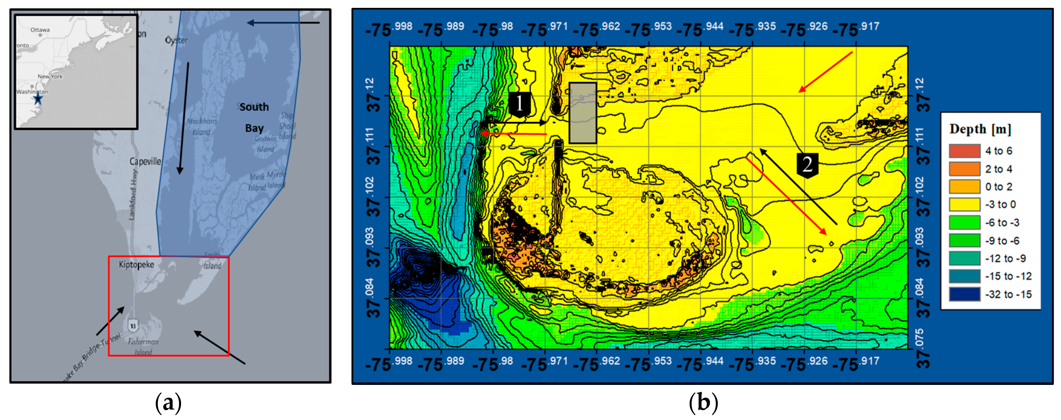
1.3. Site Description

The Chesapeake Bay is the largest estuarine ecosystem in the United States stretching 195 miles inland from the coast of Virginia and Maryland on the east coast of the United States, as shown in Figure 1. The estuary has a relatively shallow depth that experiences moderate mixing between salt and fresh water from the north to the south of the estuary. It experiences a semi-diurnal tidal cycle whose range varies between 0.5 m to 1 m at the mouth. The main channel is 5 km to 7 km wide, 23 m deep, and is bordered by marsh and two major cities (Baltimore and Washington D.C.) [30]. The position of this main navigational channel is shown in Figure 1a to the left of the Eastern shore Project site indicated by the red box. At the mouth of the Chesapeake Bay another smaller bay called the South Bay can be seen accented in blue to the right of the Eastern Shore Project site shown in Figure 1a. Unlike the Chesapeake Bay, this bay is dominated by marshland and is bordered by a system of barrier islands. The Eastern Shore Project site is located between the mouths of these two regions, which is outlined in red in Figure 1a, with the instrumented marsh indicated by the gray box in Figure 1b.

There are two main inlets that contribute to the hydrodynamic forcing at the Eastern Shore Project site, indicated by the numbers 1 and 2 in Figure 1b. Waves penetrate through these two inlets generated in the Atlantic by offshore storms, which can vary from seasonal storms to category four hurricanes. Therefore, the wave climate oscillates between swell and locally generated wind waves; however, the relatively shallow bathymetry prevents waves above inlet 2 from penetrating to the site unless a high enough storm surge is present. Inlet 1 has a gentle slope of 0.6 percent, transitioning from a depth of 7 m to 1 m over 1 km. The incoming wave climate approaches from the main channel but has a majority of its energy dissipated through breaking just outside the Eastern Shore Project site as a result of the aforementioned slope, and resulting shallowness of the Eastern Shore Project site. Inlet 2 transitions from a depth of about 7 m to 2 m over a length of 2 km, resulting in a very gentle slope of 0.2 percent. Inlet 2 is open to offshore wave conditions but like inlet 1 this incoming wave climate sees a majority of its energy dissipate through breaking as a result of the slope and shallowness.

Similar to the mouth of the Chesapeake Bay, the Eastern Shore Project site experiences a semi-diurnal tide cycle with a tidal range varying between 0.5 m to 1 m. With the most landward portion of the site lying 1 m above mean sea level, the site is only partially inundated during high spring tide and is completely dry during low spring tide. During the transition from flood to ebb, the dominant flow to the research site enters from the mouth of the South Bay indicated by the red arrows in Figure 1. The flow continues around Raccoon Island and exits through inlet 1, into the main channel of the Chesapeake Bay.

The project site is covered by Spartina Alterniflora, a saltmarsh plant found commonly along the eastern coast of the United States. The wider area also consists of deciduous coastal forest, coastal shrubland and coastal grassland. These various vegetation types each contribute to the mitigation of flood hazards impacting the surrounding community.

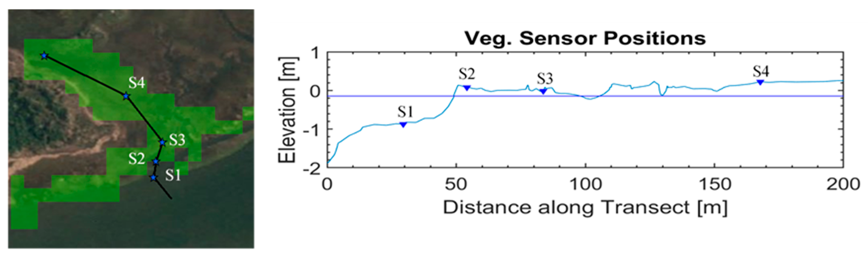
1.4. Data Description

The field data is recorded using 4 Trublue 255-70530 pressure gauges set along the marsh from the leading edge to the rear. These pressure gauges provide temperature (Celsius) and pressure (PSI) readings, taken at intervals of a 0.25 s from 24 September to 2 October of 2015. The gauges have an accuracy of ±0.5% FS TEB with a resolution of 0.01% FS or better (FS meaning full scale or difference between the highest and lowest measurement, and TEB means total error band which includes errors due to non-linearity, hysteresis, non-repeatability and thermal effects). The pressure time series is converted to a water level time series where the significant wave heights (Hs) and periods can be extracted through spectral analysis. These results are then used to validate the model. Figure 2 shows the position of the Trublue sensors on a transect crossing the research site, both horizontally and vertically.

Bathymetric data, as described in [31] is also used in the present study. Additional data was also collected at the research site on topography and vegetation, by means of surveys. The bathymetric and topographic features are provided at a resolution of 5 m. The vegetation is sampled at 8 different positions along a transect across the marsh shown in Figure 2, below. High-resolution bathymetric data was also required for the larger nearshore domains, this was provided by means of a high-resolution Virginia Beach Digital Elevation Model [32].

GEBCO data was used for open ocean bathymetry [33]. National Oceanic and Atmospheric Administration (NOAA) wave data using moored buoys along the coast of the United States [34] is used to validate the regional model results. Regional model tide data was provided by the TPXO7.2 tidal model [35]. Landcover data used in the SWAN standalone model to identify vegetation cover at the research site which was provided [28].

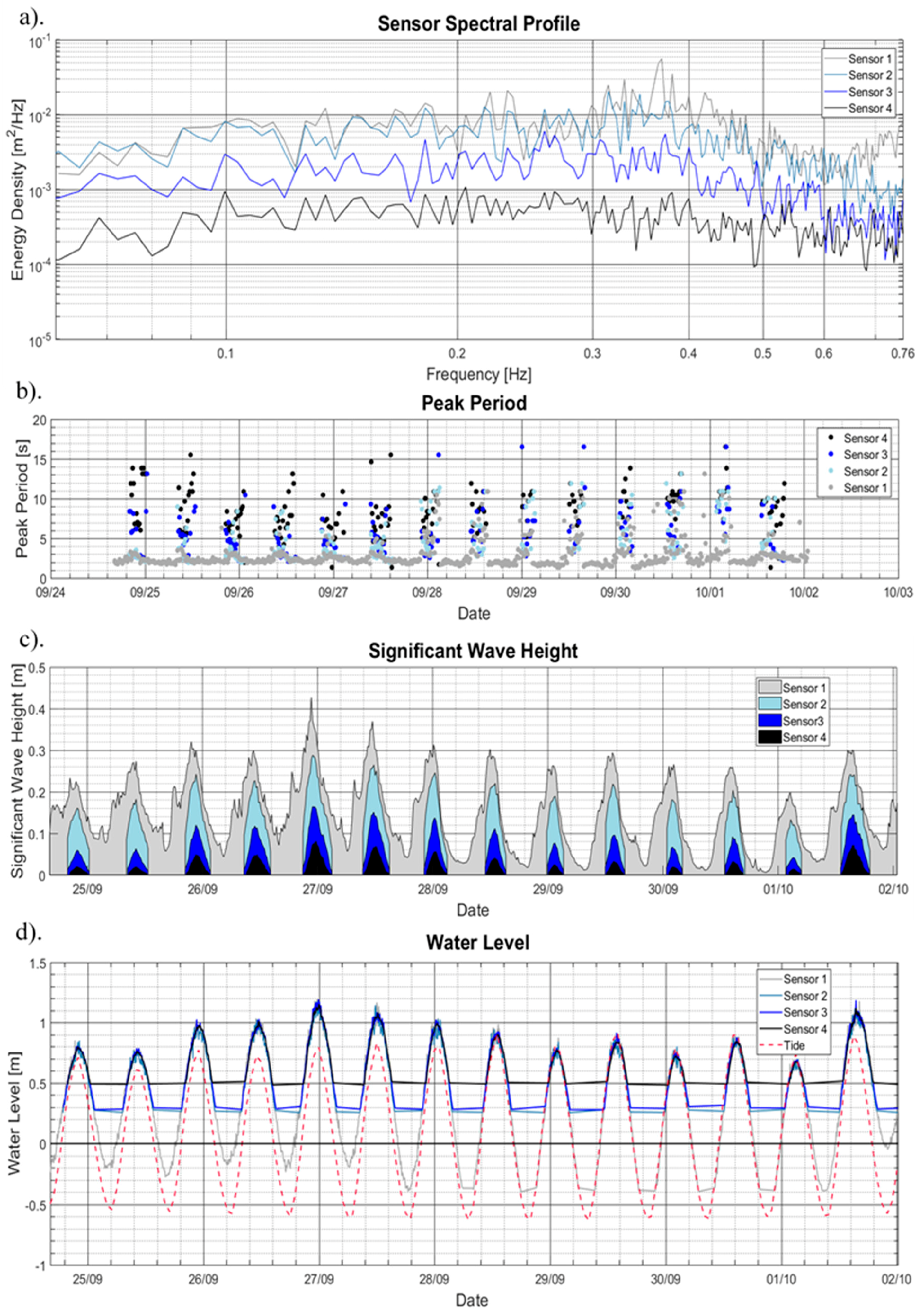
1.4.1. General Wave Climate

Figure 3 shows the wave climate recorded by the four Trublue pressure sensors on the marsh. Figure 3a show a decrease in wave energy across all frequencies from sensors 1 to 4, with most of the energy focused between 2 Hz to 5 Hz. This indicates a locally generated wind wave climate entering the marsh at sensor 1. Figure 3b indicates a transition of the Tp range from 2 s–10 s to 2 s–16 s, suggesting a transition of wave energy from high to low frequencies. Figure 3c shows a range of Hs from 0.02 m to 0.42 m, with the peak wave height occurring on 27 September. During the time of interest, the wave heights are reduced by about 80% from sensor 1 to sensor 4. Figure 3d shows the water levels recorded at the marsh about the NAVD88 vertical datum as well as the tide cycle during this time. The storm surge is the difference between the water level and the astronomical tide. Like the Hs the peak water level occurs during 27 September where it reaches 1.15 m resulting in a storm surge of about 0.4 m. From Figure 3b–d there are gaps in the wave data caused by cutoffs applied at points where the water levels are too low for the pressure sensors to reliably record accurate data. The cutoff applied for sensors 1 to 3 are 0.3 m above the vertical datum; for sensor 4 the cut off is applied at 0.5 m above the vertical datum.

1.4.2. Wind

Wind and sea level air pressure are provided by the ECMWF (European Center for Medium range Weather Forecast) atmospheric operational model. The data provided by the ECMWF encompasses the whole of the Gulf of Mexico as well as part of the Atlantic Ocean just off the east coast of the United States. The grid has a 0.141 degree or 15.5 km north–south and a 12.5 km east–west resolution with a time step of 6 h between each wind velocity and pressure reading [36]. The local accuracy of this wind model was verified by Garzon et al. [37]. The ECMWF winds were compared with local weather stations, the highest correlation occurred at the mouth of Chesapeake Bay where it reached over 95% correlation to station data [37].

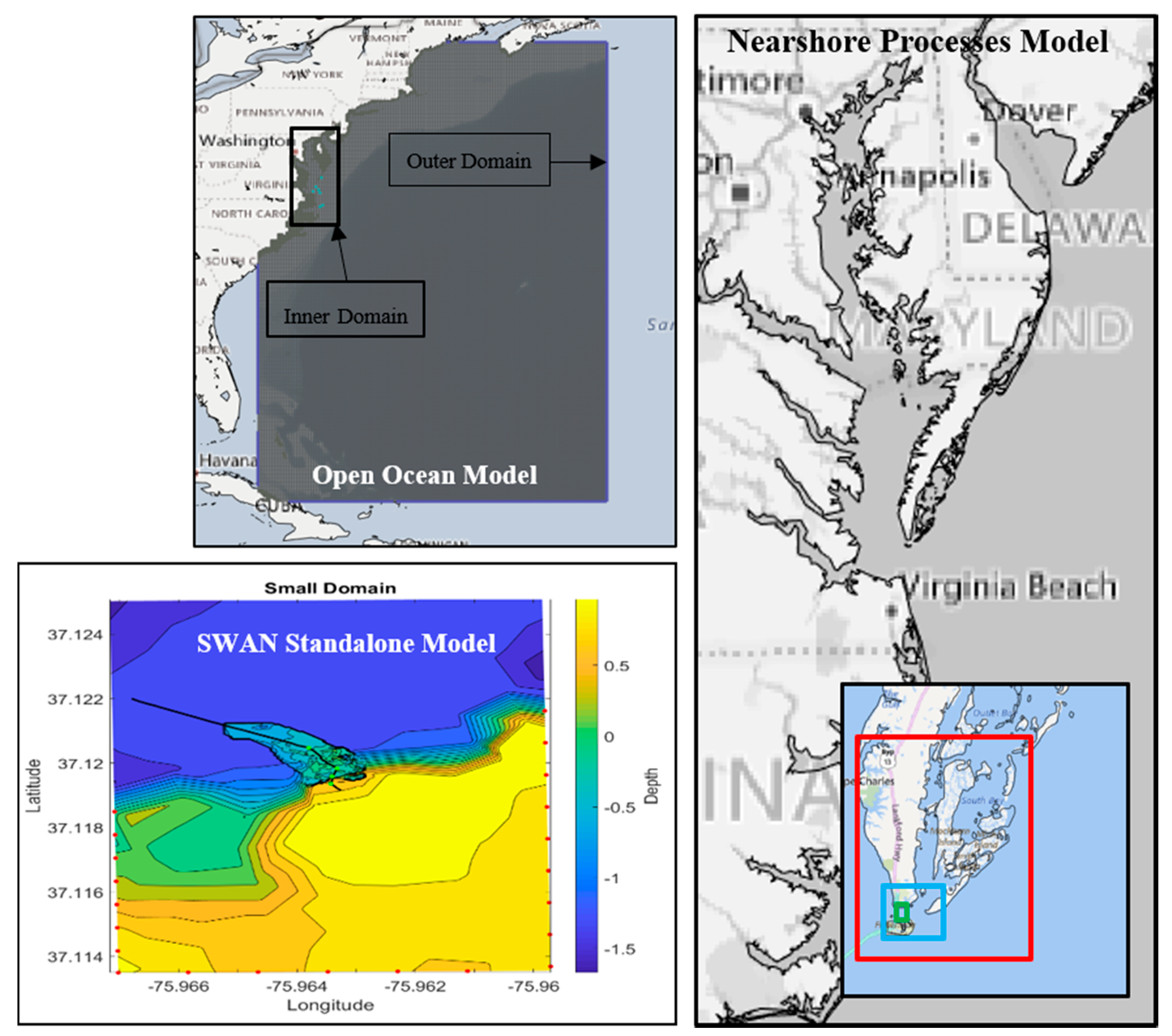
2. Modeling Approach

In order to run the SWAN standalone model (SSAM) for the study area, boundary conditions needed to be determined. This was done through the creation of a Delft 3D Flow + Wave model that recreates the necessary offshore and nearshore wave conditions. This Methodology section is therefore broken down into three parts, each describing the models mentioned above. These parts include: (i) the largest (2120 km by 2483 km) Open Ocean model (OOM), whose purpose is to recreate offshore wave climate and storm surge due to meteorological forcing; (ii) the Nearshore Processes Model (NPM), which refines portions of the OOM to recreate the nearshore processes necessary to produce boundary conditions; and (iii) the SWAN Standalone model (SSAM), which uses the boundary conditions produced by the NPM to assess the vegetation representations.

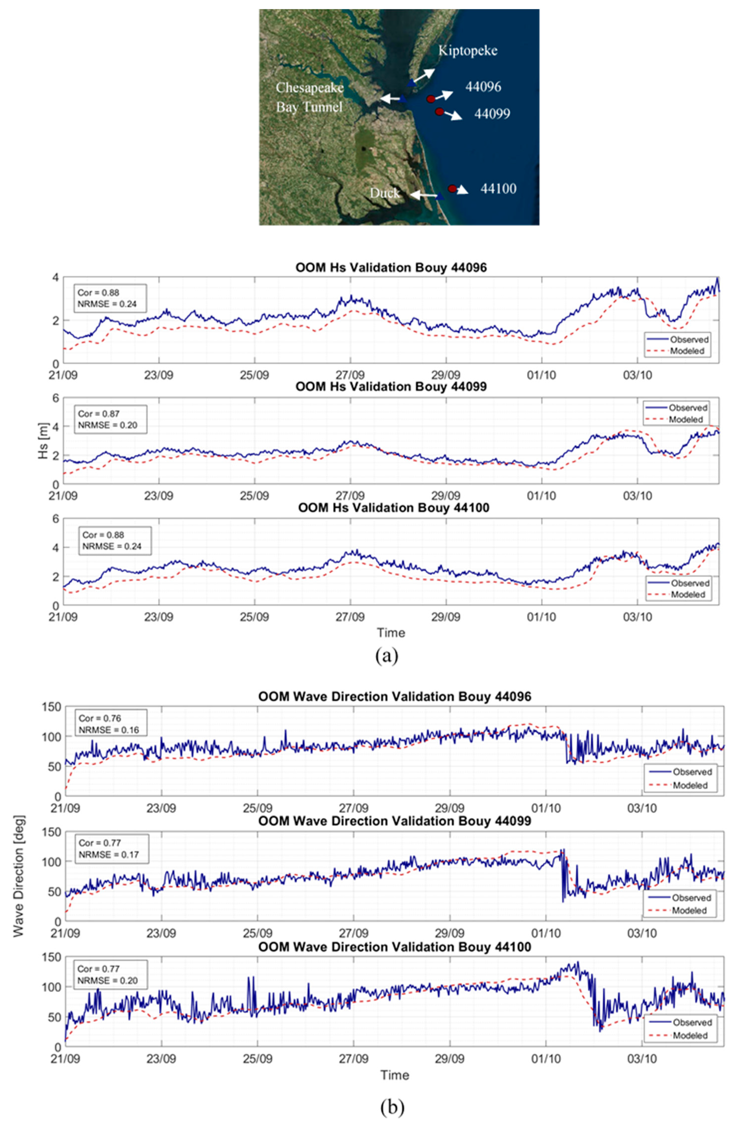
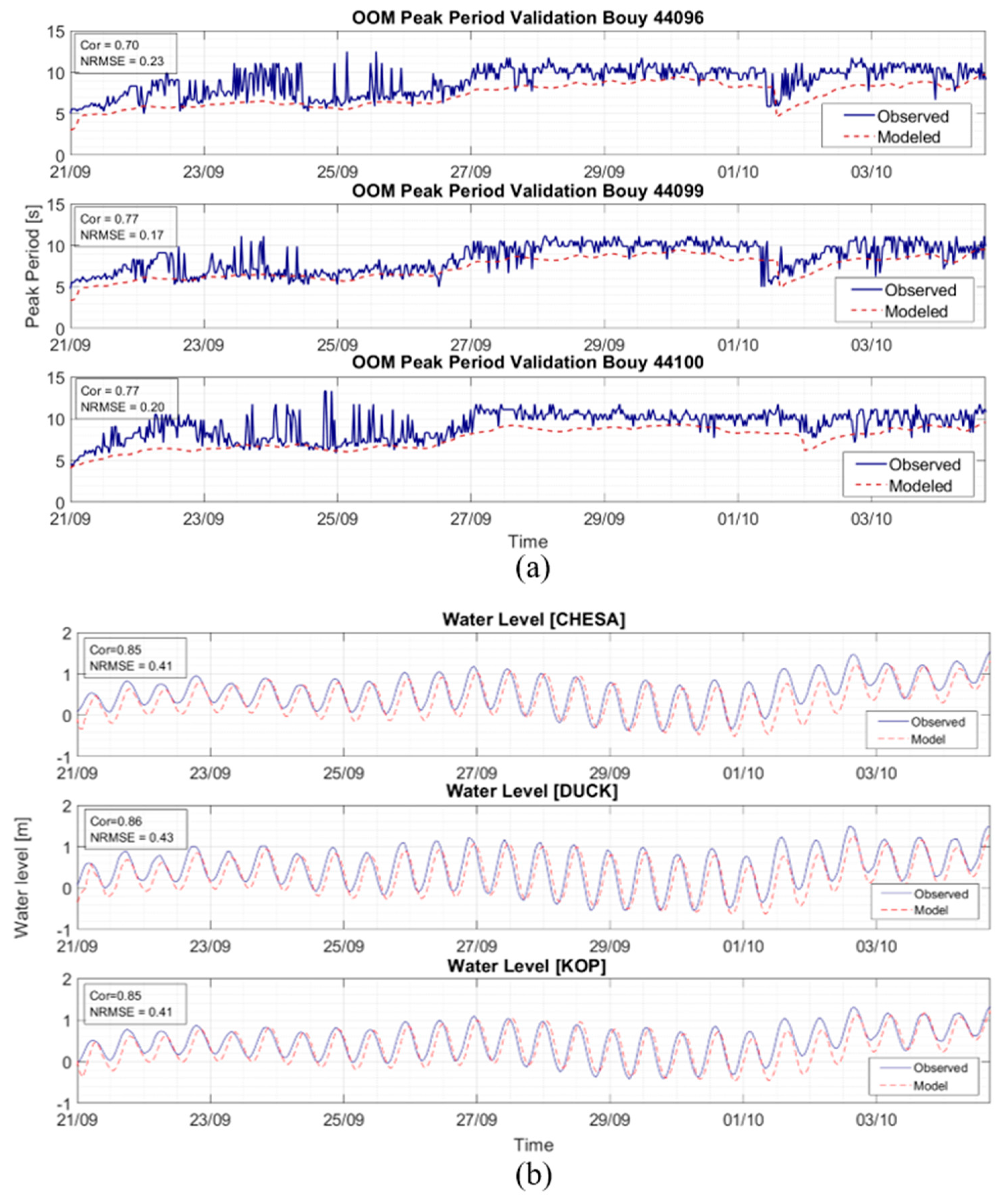
2.1. Open Ocean Model (OOM)

The OOM model was created in Delft3D Flow + Wave modules using the meteorological data, GEBCO bathymetry and TPXO7.2 tide data [35]. The Delft 3D Flow and Wave modules were two-way coupled, meaning that the Wave module passed information on radiation stresses to the Flow module, and the Flow module passed information on water depth and flow speed to the wave module [38]. The time step for this computation is set to 10 min with the coupling interval set to 60 min. Riemann boundary conditions are selected for this model in order to minimize reflection.

The final setup of the OOM model consists of two computational grids shown in Figure 4, a 0.075-degree (8.25 km) resolution outer domain and a 0.015-degree (1.6km) resolution inner domain (which was decomposed from the larger grid), three 0.141-degree equidistant meteorological grids, and 0.008 degree (0.9 km) bathymetric grid. The time step is set at 12 s and the simulations cover 15 days, starting on 20 September 2015 and ending on 5 October 2015. The bottom friction for the wave module uses the JONSWAP formulation with a roughness coefficient of 0.06 to indicate a wave climate between swell and wind sea states [39,40]. The wind drag values were adjusted to 0.001 and 0.002 as a result of calibration which indicated that lower wind drags resulted in more accurate modeled peak periods. The formulation for wave dissipation by whitecapping (deep-water wave breaking) was changed from the Komen et al. [41] formulation to the Van der Westhuysen et al. [42] formulation for the same reason, as suggested in [42].

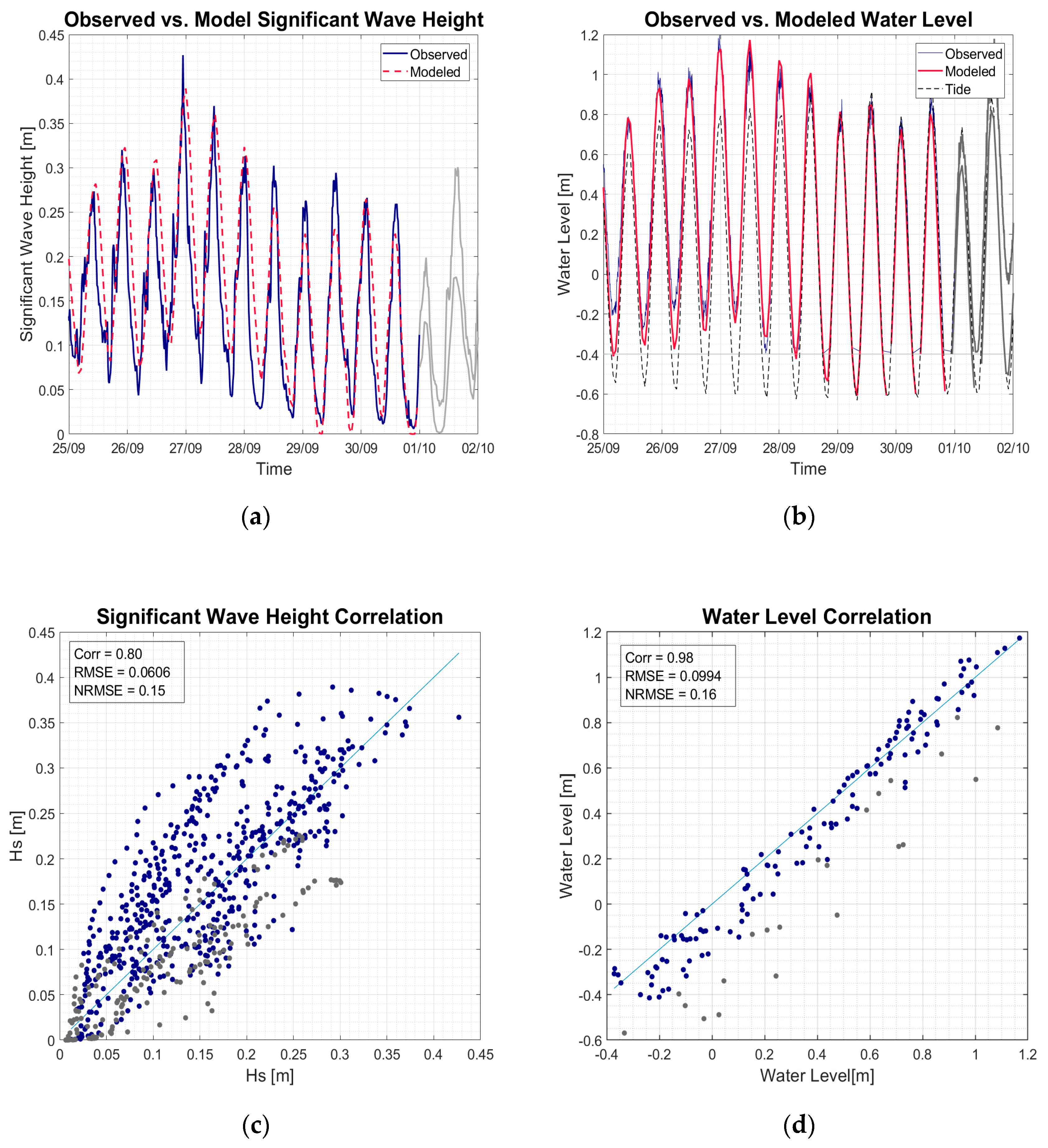
2.2. Nearshore Processes Model (NPM)

After the completion of the OOM, its inner domain was broken down into three increasingly smaller domains. Each domain is reduced by a factor of 5—relative to the preceding domain size—until a near 5-m resolution is achieved, to match that of the SSAM. The NPM is forced by the OOM, therefore, all physical processes are the same. However, parameters such as the manning roughness for the flow module and the breaker parameter, which controls the ratio of breaking waves to local water depth, were adjusted to calibrate the model because it had been too dissipative, resulting in larger errors for the water levels. The bottom roughness for the flow module, specified here using Manning n, is therefore set to 0.015. The SWAN breaker parameter was set to 0.5 due to the shallow and relatively flat characteristics of the research site, as discussed in [43,44]. These regions required finer bathymetry which was provided by the data discussed in Section 2.1.

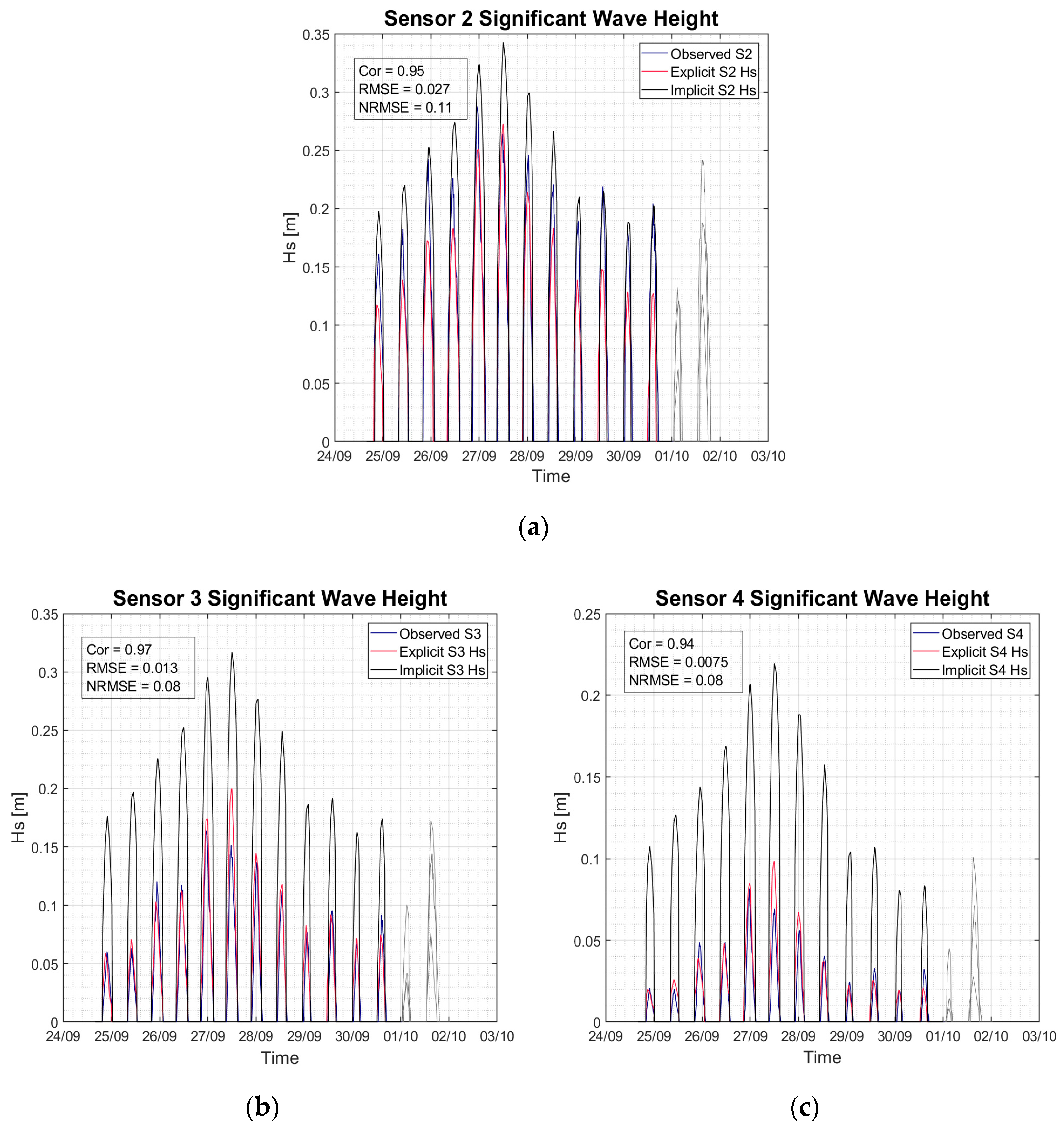
2.3. SWAN Standalone Model (SSAM)

From the NPM, boundary conditions for the SSAM are extracted as spectral data (.sp2) for 20 observation points. These points provided the wave characteristics necessary to run the SSAM. The NPM was also used to create water level, current velocity and wind velocity fields that were applied to the SSAM.

The land cover file used for the explicit vegetation implementation in SWAN takes advantage of the “NPLANTS” command to create vegetation cover of varying density. The landcover file indicates that the vegetated regions have a uniform density equivalent to 100% of the density provided by the SWAN command file. The vegetation height, density and diameter are all specified to match those observed in the field [31]. These values were averaged and applied as constant values across the marsh (density: 344 stems/m², vegetation height: 0.71 m and diameter: 5.2 mm).

The selection of the drag coefficient for the explicit representation is based on three formulations; the first of which was proposed by Méndez et al. [10], demonstrated in Equation (8), which was determined through laboratory experiments using flexible plastic strips to represent the vegetation.

$$C_D={\frac{2200}{Re}}^{2.2}+0.08$$

(8)

where Re is the Reynolds number, determined as a function of velocity, stem diameter, viscosity and density. The second formulation is that of Jadhav and Chen [45],which was determined from field observations taken during a tropical cyclone shown in Equation (9).

$$C_D=\frac{2600}{Re}+0.36$$

(9)

The final formulation was determined using the drag relation discussed by Smith et al. [19], who used synthetic Spartina Alterniflora in a laboratory experiment to produce Equation (10).

$$C_D={\frac{744}{Re}}^{1.27}+0.76$$

(10)

Unlike Equation (8), both Equations (9) and (10) were developed with field data of Spartina Alterniflora plants. Since the vegetation species is constant throughout the marsh, the diameter does not change significantly; however, the velocity—used to determine Re—is strongly dependent on the wave climate. Therefore, to determine which current velocity best represents the 20 September to 6 October wave climate largest, smallest, and average current velocities that occur at the Eastern Shore research site are used to determine the Re. The current velocity during the period of interest varies from 0.1 m/s to 0.7 m/s giving a range of Re values from 430 to 5000.

For the implicit vegetation representation, a second land cover file uses Equation (3) to determine K_N values for the different portions of the marsh. These are implemented in SWAN using the Madsen bottom friction formulation (Equations (3)–(6)), effectively implementing the Manning “n” as an adjusted friction length.

Both files require the identification of vegetation types in the region. The vegetation was identified using the Virginia Gap land cover data [28]. This dataset classifies many land cover types into their own classification and presents them on a map that encompasses the entire United States. This data showed that the research site was completely covered by saltmarsh, which has an n value of 0.035 [46].

3. Results

The OOM results are validated using observed data provided by the National Oceanic and Atmospheric Association [34]. These buoys and tide stations provide the Hs, Tp, wave direction and water level between 20 September and 6 October, 2015. The NPM, as well as the SSAM, are both validated using the Trublue pressure sensor data shown in Figure 3.

3.1. Open Ocean Model

The NOAA buoy and tide station data used to validate the OOM is shown in Figure 5 and Figure 6 along with their corresponding correlation coefficient and normalized root mean squared error. Figure 5a,b show the comparison of the Hs and Wave direction. The model recreates the Hs with the largest correlation of 0.88 occurring at buoys 44096 and 44099 and the smallest NRMSE of 0.20 occurring at buoy 44099. The highest correlation of 0.77 for wave direction is achieved at buoys 44099 and 44100 with buoy 44096 achieving the lowest NRMSE of 0.16. Figure 6a,b show the comparison between the peak period and the water level. The model recreates the observed peak period with the highest correlation of 0.77 occurring at buoys 44099 and 44100 and the lowest NRMSE of 0.17 occurring at buoy 44099. The model water levels in Figure 6b achieve a correlation of 0.86 and NRMSE of 0.41 with the observed buoy data.

3.2. Nearshore Processes Model

Like the OOM, the Domain Decomposition model adequately recreates the observed wave heights (Figure 7), with a correlation coefficient for Hs of 0.8 with a 0.15 normalized root mean square error. The water levels correlation coefficient is 0.98, with a normalized root mean square error of 0.16. The NPM correlation reveals that the model consistently underestimates the lower water levels (Figure 7d). The model also underestimates larger wave heights while overestimating the smaller wave heights.

3.3. SWAN Standalone Model Validation & Comparison

The validation for the SSAM is shown in Figure 8 along with the correlation for the explicit representation. When comparing the SSAM results to the observed data, it is evident that the explicit vegetation representation more accurately replicates the wave attenuation by the saltmarsh (Figure 8). Although at the first sensor the accuracy is not as distinguishable as it is at the forth sensor. The explicit representation achieves a correlation of 0.73 at sensor one which increases to 0.95, 0.97 and 0.94 from sensors 2 to 4 respectively. The normalized root mean square error for sensors 1 to 4 are 0.18, 0.11, 0.08 and 0.08. The implicit vegetation representation achieves correlation coefficients of 0.92, 0.91, and 0.90 and normalized root mean square errors of 0.36, 0.89 and 0.96 for sensor 2, 3 and 4, respectively.

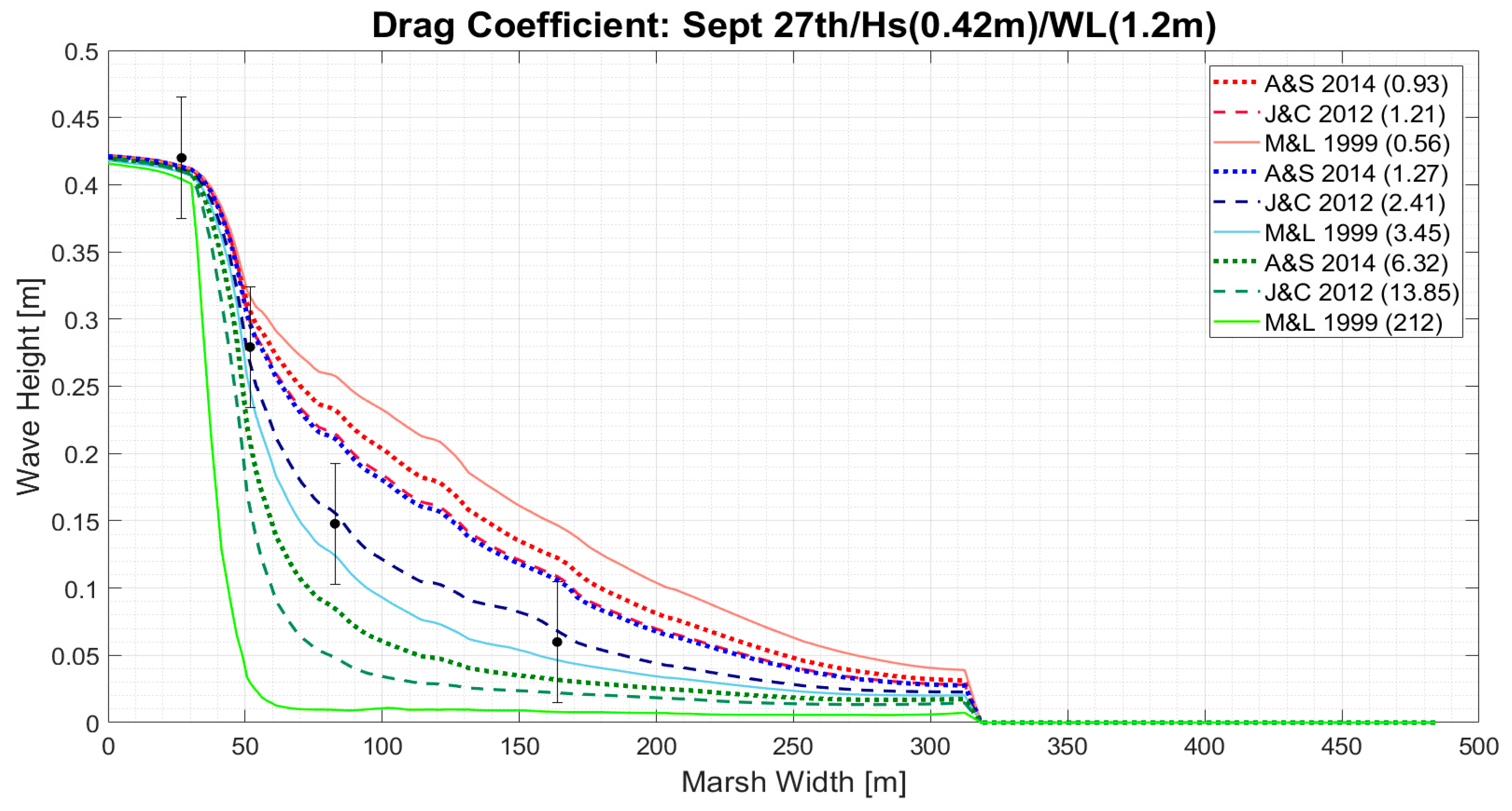
3.3.1. Explicit Representation: Drag Coefficient Profiles

The highest water levels and wave heights were recorded at the marsh on 27 September of 2015, and therefore, our analyses will focus on this period. The three current velocities used to determine the drag coefficients are indicated in Figure 9 and are 0.1 m/s (red), 0.29 m/s (blue) and 0.7 m/s (green). The most accurate results were created using the Jadhav and Chen 2012 [37] drag formulation with the average current velocities indicated by the dashed dark blue line in Figure 9. In general, the Hs is reduced by approximately 40% at 50 m into marsh and 80% at 160 m into marsh. Looking at Figure 9, the lower drag forces representing the higher current velocities shown in red perform the best at the front edge of the marsh while the lowest velocities perform the best at the back end of the marsh.

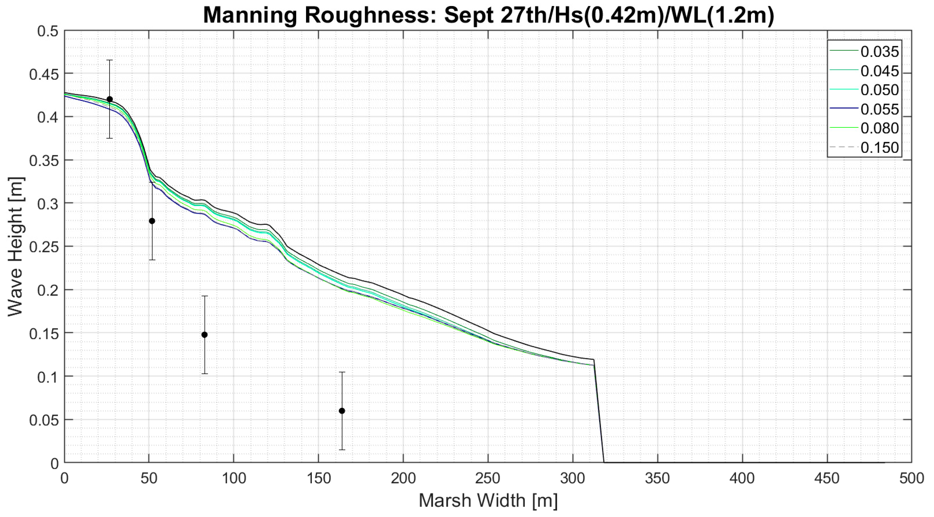
3.3.2. Implicit Representation: Manning Roughness Coefficient Profiles

The model showed a very small sensitivity to the use of Manning roughness coefficient shows the wave dissipation for manning roughness values that were varied from 0.035 to 0.150 (Figure 10). Very little change occurs, with the most accurate results occurring in the first 50 m, where vegetation is not present over the entire region. The wave height is reduced by 20% over the first 50 m when using the manning approach, eventually reducing the wave height by 50% in the first 160 m.

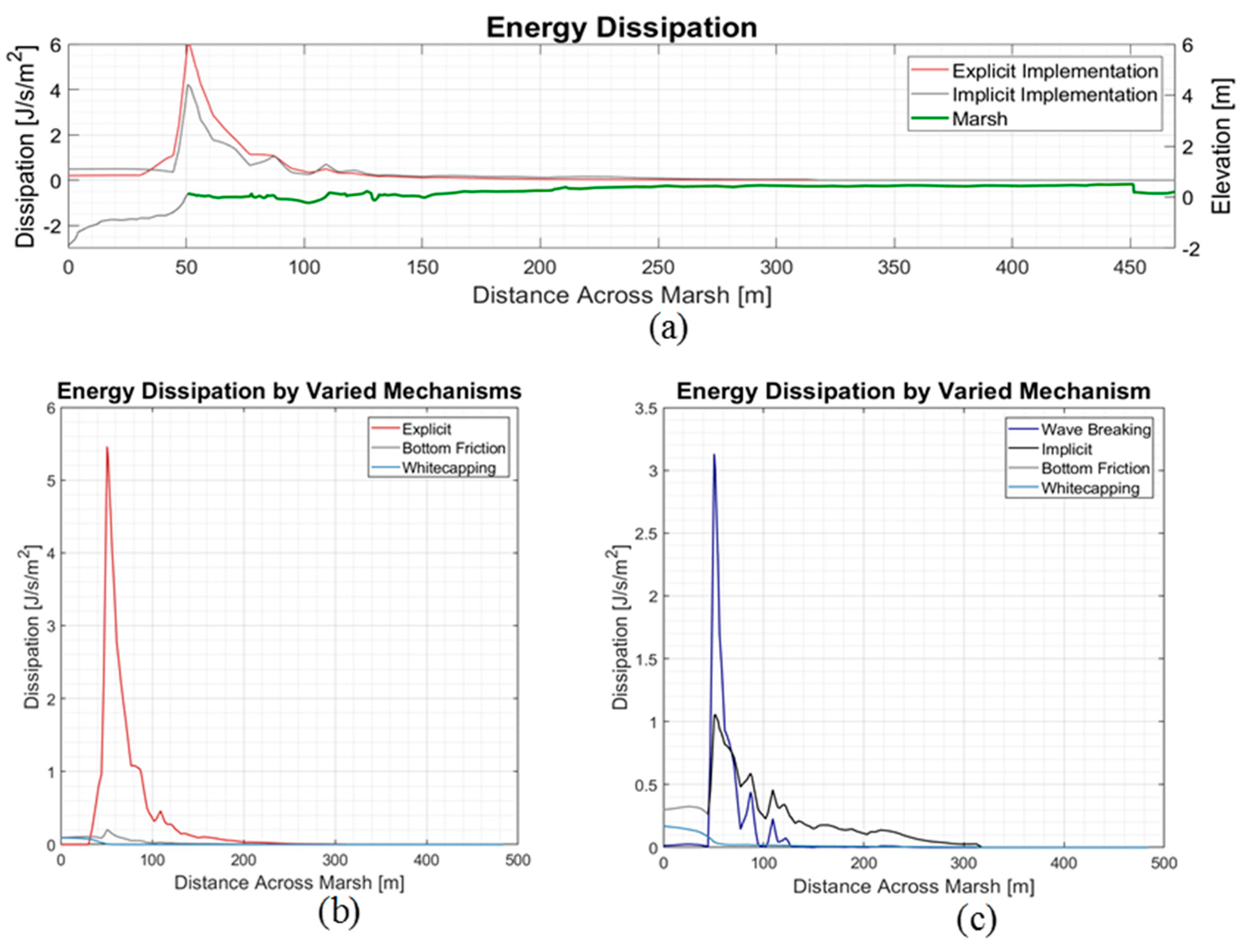
3.3.3. Wave Energy Dissipation Processes

Figure 11 shows the energy dissipation rates across the marsh for both the implicit (gray) and explicit (red) vegetation representations. Both profiles show a region of significant dissipation occurring at the leading edge of the marsh; around 50 m into Figure 11a. The Implicit representation produced a dissipation of 4.2 J/s/m² while the Explicit representation produced a dissipation of 5.8 J/s/m². This occurred in the breaker area where a large fraction of the energy dissipation is taking place. Figure 11b,c separated the energy dissipation process into their associated dissipation mechanisms. Figure 11b shows the explicit run which experienced dissipation by whitecapping, bottom friction and explicit vegetation dissipation. Figure 11b shows that the Implicit run experienced dissipation by bottom friction, the implicit vegetation, whitecapping and other forms of wave breaking.

In the implicit run, wave breaking produces the highest dissipation rate at 3.1 J/m/s² at the beginning of the breaker region but is then overtaken by the dissipation due to the implicit vegetation at around 30 m from the leading edge of the marsh shown in Figure 11c (presence of vegetation shown in green). The implicit vegetation produces a peak dissipation rate of 1.1 J/m/s² in the breaker region and continues further into the rear of the marsh than the wave breaking, which dominated the first 30 m.

The explicit run, on the other hand, is completely dominated by dissipation due to vegetation where the peak dissipation rate of 5.4 J/s/m² is experienced in the breaker region. Dissipation by bottom friction is experienced at a peak rate of 0.1 J/s/m², much smaller than the implicit run. However, like the implicit run, the explicit run also showed whitecapping in the offshore portion in front of the marsh, which is completely overtaken by other dissipation mechanisms shoreward of the marsh edge.

The main difference between the two runs is the role that wave breaking plays in the implicit run when compared to the explicit run. By excluding the influence of the various vegetation properties on wave attenuation (implicit representation), waves are able to retain their energy further shoreward resulting in intense wave breaking over the first 50 m of marsh (Figure 11b). On the other hand—with the explicit representation—the waves experience significant attenuation by vegetation; such that the breaking criteria (ratio of breaking wave height to water depth) is not violated and, thus prevents intense wave breaking (Figure 11a) [2].

4. Discussion

This section will discuss the validation of the OOM and NPM models as well as the comparison between the implicit and explicit representations. Section 4.1 briefly describes the observed trends of the three models and how they manifested themselves from the OOM model to the SSAM. Section 4.2 focuses on the difference in wave dissipation rate and dissipation mechanism between the two implementations. The results are also compared to existing research to identify how this paper compares the current work.

4.1. Model Calibration and Validation

The OOM model was able to recreate the observed wave climate with reasonable accuracy but showed a tendency to underestimate the significant wave heights, peak periods and water levels. To alleviate this issue whitecapping, computational grid resolution, bathymetric grid resolution and wind drag were adjusted through sensitivity analysis, producing the results shown in Figure 5 and Figure 6.

The adjustment of the whitecapping from the default formulation of Komen et al. [41] to that of Van der Westhuysen et al. [42] was done because the findings in [42] indicated an underestimation of peak periods in mixed wind and swell sea states when using the Komen et al. [41] formulation. This indicates that the wave climate is a mixed sea state whose energy distribution is impacted by the presence of whitecapping in the model which demands a reasonable amount of attention.

The refining of the bathymetric and computational grids to 0.015 degrees improved the results, indicating that key bathymetric features were not captured when a coarser grid resolution of 0.075 was used. There were also 1- to 2-m differences in depth which can impact the extent to which bottom friction and wave breaking affect the development of the incoming wave climate.

The wind drag also proved to have major impact on the peak periods, with lower wind drag coefficient values such as the 0.01 and 0.02 producing larger peak periods. The wind drag influence how much energy is transferred across the wind sea interface as well as the celerity of the incoming wave climate. The wind drag and whitecapping are also interconnected within SWAN, magnifying the influence the wind drag has on the peak period.

The underestimation of water level and significant wave height, observed in the OOM, was minimal in the NPM (Figure 7). However, the NPM model showed difficulty in recreating the observed spectral profile (Figure 12). As shown in Figure 12, the numerical model transfers an excessive amount of energy to higher frequencies while neglecting energy transfer to lower frequencies, as the water depth becomes shallower. This is seen from the Inlet shoreward, where the modeled spectra show a peak forming at ~0.4 Hz (at the center) which migrates to 0.5 Hz (at the Boundary). This results in an overestimation of wave energy at higher frequencies compared to the observed data at Sensor 1 (Figure 12).

It is also possible that the underestimation of the peak period in the OOM model is translating to the error in spectral profile, however at the Eastern Shore Project site new factors, such as triad wave–wave interactions and the ratio of breaking waves to local water depth (breaker index), become more influential to the development of spectral profiles due to the shallowness of the NPM when compared to the OOM. Therefore, it is necessary to further study the development of the spectral profile in this region.

These factors are a fraction of a large group of variables that can influence the final wave characteristics of the OOM and NPM. The number of variables calibrated in these models are a testament to the complexity of the wave generation and propagation process. Due to the complexity of these processes, numerical models will rarely be able to perfectly recreate observed wave climates. Regardless, the OOM and NPM models have demonstrated that these tools can be used to model bulk parameters such as significant wave height and water levels to a NRMSE below 20%, which is beneficial to further assessment of the Chesapeake Bay coastal region.

4.2. Explicit Versus Implicit Vegetation Representations

The SSAM was able to appropriately recreate the observed wave climate across the marsh using the explicit vegetation implementation (Figure 9) but significantly less so when the implicit representation was used (Figure 10). Along with general performance, the two vegetation representations produced different wave dissipation mechanisms which can be very important when considering the morphological stability of the marsh. The minor errors in the explicit representation may be attributed to the constant drag coefficient and vegetation characteristics, which are not representative of real-world conditions where these variables vary horizontally and vertically across the marsh. The significant overestimation of significant wave height in the implicit representation, on the other hand, suggests that treating vegetation dissipation as merely enhanced bottom friction ignores the more complex processes occurring throughout the water column, as discussed in [11]. A more detailed discussion of the two implementations are presented below.

For the explicit representation, SWAN performed the best when using the Jadhav and Chen [45] drag coefficient formulation and the average current velocity of 0.29 m/s (Figure 9). This finding differs from that of Vuik et al. [2], who found that the Méndez et al. [10] formulation resulted in a better agreement with their observed field data. In the present study, [10] is the second-best fitting drag coefficient for the observed field data. Both the forcing and vegetation details differ between this study and [2]. The vegetation present in [2] is submerged, similar to the vegetation present in the laboratory experiment where [10] was derived. Jadhav and Chen [45] shared similar forcing and vegetation characteristics to the Eastern Shore Project site, it therefore may be more appropriate to recreate the observed filed data, as shown in Figure 9.

Additionally, the drag coefficient was held constant throughout the marsh which, though relatively accurate, is not representative of real-world conditions. As presented in Section 2.3, the drag coefficient is a function of the Reynolds number which itself is a function of current velocity. Current velocity is not naturally constant and can be influenced by vegetation density, vegetation height and water depth as describe in [11]. Neumeier and Amos [11] observed that vegetation characteristic vary based on wave forcing, from the front to the back of the marsh; which was observed in the vegetation data of the Eastern Shore Project site, shown in [31]. These characteristics influence the vertical and horizontal rate of change in the current velocity, the development of boundary layers, and creation of free streaming regions [11], all of which can impact the dissipation rate.

For the implicit representation, the Manning “n” values of 0.055, 0.080 and 0.150 performed the same. This is likely caused by the limit placed on the friction factor formulation applied in SWAN, as discussed in [20]; overcoming this limitation would require an adjustment of the source code in order to change the friction factor formulation to that of [47]. However, it is important to note that the formulation used in [20] was implemented for fully submerged sea grass which behaves differently to the emergent vegetation observed at the Eastern Shore Project site. An n value of 0.055 was ultimately chosen as the appropriate value for the implicit representation because it represents marsh vegetation, whereas the other two represent coastal shrubs (n = 0.080) and coastal forest (n = 0.150).

When comparing the explicit Jadhav and Chen [45] drag formulation (Figure 9) and the implicit Manning, n = 0.055 (Figure 10), the explicit representation outperforms. Both implementations had high correlation coefficients across the marsh but differed greatly in NRMSE. While the explicit representation maintains a NRMSE below 0.15 (or 15%) from sensors 2 to 4, the implicit representation produced NRMSE that exceeded 0.30 from sensor 2 to 4. These results showed that the implicit representation, using the SWAN default friction factor formulation, cannot adequately recreate the wave dissipation produced by emergent marsh vegetation. The magnitude of the bottom friction applied through the implicit representation is not large enough to appropriately mimic the vertically and horizontally varied drag forces across the marsh.

Figure 11 showed that the representations not only differed in the magnitude of wave dissipation but also in the dissipation mechanisms they produced. While the explicit representation showed that a majority of the wave energy is being dissipated by the vegetation throughout the marsh, the implicit representation is initially dominated by wave breaking at the leading edge of the marsh. The vegetation does become the dominant from of dissipation once the flatter parts of the marsh are reached, but the amount of dissipation that the vegetation is responsible for in the implicit representation is a small fraction of that in the explicit representation.

These characteristics can be observed in [2,20] who also separated the breaker mechanisms present on marsh lands. The dissipation mechanisms in the implicit representation more closely resembles a mud flat than a salt marsh, which can also be seen in [2] who conducted a similar break down for an unvegetated region. These dissipation mechanisms can become important when assessing the morphological changes of a salt marsh and should be considered when conducting this type of modeling.

5. Conclusions

The results showed an under performance by the implicit representation of vegetation when compared to the explicit representation, when using the default Manning-based friction factor formulation currently implemented in SWAN, corroborating the findings of Smith et al. [19] and [20]. The inability for the implicit representation to produce a friction factor large enough to fully recreate the magnitude of dissipation produced by densely vegetated marsh limits its applicability in modeling these regions. Furthermore, the implementations produced different types of dissipation mechanisms which may influence the modeling accuracy of morphological models in coastal regions. The work done in this paper is a first step in a wide range of analysis that can be carried out. Further assessment is needed on the friction factor implementation, in order to determine whether the improved performance by the implicit representation observed in [20] holds true for emergent vegetation. This would shed light on where the limits of this implementation lie, and provide guidance to coastal engineers who apply numerical modeling to investigate vegetated intertidal areas.

References

1. Zhang, K.; Liu, H.; Li, Y.; Xu, H.; Shen, J.; Rhome, J.; Smith, T.J., III. The role of mangroves in attenuating storm surges. Estuar. Coast. Shelf Sci. 2012, 102, 11–23. [Google Scholar] [CrossRef]
2. Vuik, V.; Jonkman, S.N.; Borsje, B.W.; Suzuki, T. Nature-based flood protection: The efficiency of vegetated foreshores for reducing wave loads on coastal dikes. Coast. Eng. 2016, 116, 42–56. [Google Scholar] [CrossRef]
3. Camfield, F.E. Wind-Wave Propagation Over Flooded, Vegetated Land; Coastal Engineering Research Center: Fort Belvoir, VA, USA, 1977. [Google Scholar]
4. Kobayashi, N.; Raichle, A.W.; Asano, T. Wave attenuation by vegetation. J. Waterw. Port Coast. Ocean Eng. 1993, 119, 30–48. [Google Scholar] [CrossRef]
5. Manning, R.; Griffith, J.P.; Pigot, T.; Vernon-Harcourt, L.F. On the Flow of Water in Open Channels and Pipes; Institution of Civil Engineers: Dublin, Ireland, 1890. [Google Scholar]
6. Wu, F.-C.; Shen, H.W.; Chou, Y.-J. Variation of roughness coefficients for unsubmerged and submerged vegetation. J. Hydraul. Eng. 1999, 125, 934–942. [Google Scholar] [CrossRef]
7. Smith, J.M. Modeling Nearshore Waves for Hurricane Katrina; Engineer Research And Development Center: Vicksburg, MS, USA, 2007. [Google Scholar]
8. Wamsley, T.V.; Cialone, M.A.; Smith, J.M.; Atkinson, J.H.; Rosati, J.D. The potential of wetlands in reducing storm surge. Ocean Eng. 2010, 37, 59–68. [Google Scholar] [CrossRef]
9. Augustin, L.N.; Irish, J.L.; Lynett, P. Laboratory and numerical studies of wave damping by emergent and near-emergent wetland vegetation. Coast. Eng. 2009, 56, 332–340. [Google Scholar] [CrossRef]
10. Méndez, F.J.; Losada, I.J.; Losada, M.A. Hydrodynamics induced by wind waves in a vegetation field. J. Geophys. Res. Oceans 1999, 104, 18383–18396. [Google Scholar] [CrossRef] [Green Version]
11. Neumeier, U.; Amos, C.L. The influence of vegetation on turbulence and flow velocities in European salt-marshes. Sedimentology 2006, 53, 259–277. [Google Scholar] [CrossRef] [Green Version]
12. Anderson, M.E.; Smith, J.M. Wave attenuation by flexible, idealized salt marsh vegetation. Coast. Eng. 2014, 83, 82–92. [Google Scholar] [CrossRef]
13. Dalrymple, R.A.; Kirby, J.T.; Hwang, P.A. Wave diffraction due to areas of energy dissipation. J. Waterw. Port Coast. Ocean Eng. 1984, 110, 67–79. [Google Scholar] [CrossRef]
14. Houser, C.; Trimble, S.; Morales, B. Influence of blade flexibility on the drag coefficient of aquatic vegetation. Estuaries Coasts 2015, 38, 569–577. [Google Scholar] [CrossRef]
15. Cavallaro, L.; Viviano, A.; Paratore, G.; Foti, E. Experiments on surface waves interacting with flexible aquatic vegetation. Ocean Sci. J. 2018, 53, 461–474. [Google Scholar] [CrossRef]
16. Luhar, M.; Nepf, H. Wave-induced dynamics of flexible blades. J. Fluids Struct. 2016, 61, 20–41. [Google Scholar] [CrossRef] [Green Version]
17. Cavallaro, L.; Re, C.L.; Paratore, G.; Viviano, A.; Foti, E. Response of posidonia oceanica to wave motion in shallow-waters-preliminary experimental results. Coast. Eng. Proc. 2011, 1, 49. [Google Scholar] [CrossRef]
18. Suzuki, T.; Zijlema, M.; Burger, B.; Meijer, M.C.; Narayan, S. Wave dissipation by vegetation with layer schematization in swan. Coast. Eng. 2012, 59, 64–71. [Google Scholar] [CrossRef]
19. Smith, J.M.; Bryant, M.A.; Wamsley, T.V. Wetland buffers: Numerical modeling of wave dissipation by vegetation. Earth Surf. Process. Landf. 2016, 41, 847–854. [Google Scholar] [CrossRef]
20. Nowacki, D.J.; Beudin, A.; Ganju, N.K. Spectral wave dissipation by submerged aquatic vegetation in a back-barrier estuary. Limnol. Oceanogr. 2017, 62, 736–753. [Google Scholar] [CrossRef] [Green Version]
21. Van Rooijen, A.; Van Thiel de Vries, J.; McCall, R.; Van Dongeren, A.; Roelvink, J.; Reniers, A. Modeling of wave attenuation by vegetation with xbeach. In Proceedings of the E-proceedings of the 36th IAHR World Congress, The Hague, The Netherlands, 28 June–3 July 2015. [Google Scholar]
22. Booij, N.; Ris, R.C.; Holthuijsen, L.H. A third-generation wave model for coastal regions—1. Model description and validation. J. Geophys. Res. Oceans 1999, 104, 7649–7666. [Google Scholar] [CrossRef]
23. Kennedy, A.B.; Chen, Q.; Kirby, J.T.; Dalrymple, R.A. Boussinesq modeling of wave transformation, breaking, and runup. I: 1D. J. Waterw. Port Coast. Ocean Eng. 2000, 126, 39–47. [Google Scholar] [CrossRef]
24. Theophanis, V.K.; Nigel, P.T. Breaking waves in the surf and swash zone. J. Coast. Res. 2003, 19, 514–528. [Google Scholar]
25. Viviano, A.; Musumeci, R.E.; Foti, E. A nonlinear rotational, quasi-2dh, numerical model for spilling wave propagation. Appl. Math. Model. 2015, 39, 1099–1118. [Google Scholar] [CrossRef]
26. Madsen, O.S.; Poon, Y.-K.; Graber, H.C. Spectral wave attenuation by bottom friction: Theory. In Proceedings of the 21st International Conference on Coastal Engineering, Malaga, Spain, 20–25 June 1988; American Society of Civil Engineers: New York, NY, USA, 1988; pp. 492–504. [Google Scholar]
27. Arcement, G.J.; Schneider, V.R. Guide for Selecting Manning’s Roughness Coefficients for Natural Channels and Flood Plains; US Government Printing Office: Washington, DC, USA, 1989.
28. U.S. Geological Survey. Geological Survey Gap/Landfire National Terrestrial Ecosystems; U.S. Geological Survey: Reston, VA, USA, 2016.
29. Mendez, F.J.; Losada, I.J. An empirical model to estimate the propagation of random breaking and nonbreaking waves over vegetation fields. Coast. Eng. 2004, 51, 103–118. [Google Scholar] [CrossRef]
30. Xiong, Y.; Berger, C.R. Chesapeake bay tidal characteristics. J. Water Resour. Prot. 2010, 2, 619. [Google Scholar] [CrossRef]
31. Paquier, A.-E.; Haddad, J.; Lawler, S.; Ferreira, C.M. Quantification of the attenuation of storm surge components by a coastal wetland of the US Mid Atlantic. Estuaries Coasts 2017, 40, 930–946. [Google Scholar] [CrossRef]
32. DOC; NOAA; NESDIS; NCEI. Virginia Beach Coastal Digital Elevation Model; National Oceanic and Atmospheric Administration: Silver Spring, MD, USA, 2007.
33. IOC; IHO; BODC. Cemenary Edition of the GEBCO Digital Atlas; published on CD-ROM on behalf of the Intergovernmental Oceanographic Commission and the International Hydrographic Organization as part of the General Bathymetric Chart of the Oceans: Liverpool, UK, 2003. [Google Scholar]
34. NOAA; NWS; NDBC; UD. National Data Buoy Center; National Centers for Environmental Information: Asheville, NC, USA, 1971.
35. Egbert, G.D.; Erofeeva, S.Y. Efficient inverse modeling of barotropic ocean tides. J. Atmos. Ocean. Technol. 2002, 19, 183–204. [Google Scholar] [CrossRef]
36. ECMRWF. Ecmwf’s operational model analysis, starting in 2011; Research Data Archive at the National Center for Atmospheric Research, Computational and Information Systems Laboratory: Boulder, CO, USA, 2011. [Google Scholar]
37. Garzon, J.L.; Ferreira, C.M.; Padilla-Hernandez, R. Evaluation of weather forecast systems for storm surge modeling in the chesapeake bay. Ocean Dyn. 2018, 68, 91–107. [Google Scholar] [CrossRef]
38. Manual, D.D.-F. Delft3D-3D/2D modelling suite for integral water solutions-hydro-morphodynamic s. Deltares Delft. Version 2014, 3, 34158. [Google Scholar]
39. Hasselmann, K.; Barnett, T.; Bouws, E.; Carlson, H.; Cartwright, D.; Enke, K.; Ewing, J.; Gienapp, H.; Hasselmann, D.; Kruseman, P. Measurements of Wind-Wave Growth and Swell Decay during the Joint North Sea Wave Project (JONSWAP); Ergänzungsheft 8-12; Deutches Hydrographisches Institut: Hamburg, Germany, 1973. [Google Scholar]
40. Bouws, E.; Komen, G. On the balance between growth and dissipation in an extreme depth-limited wind-sea in the southern north sea. J. Phys. Oceanogr. 1983, 13, 1653–1658. [Google Scholar] [CrossRef]
41. Komen, G.J.; Cavaleri, L.; Donelan, M.; Hasselmann, K.; Hasselmann, S.; Janssen, P. Dynamics and Modelling of Ocean Waves; Komen, G.J., Cavaleri, L., Donelan, M., Hasselmann, K., Hasselmann, S., Janssen, P.A.E.M., Eds.; Cambridge University Press: Cambridge, UK, August 1996; p. 554. ISBN 0521577810. [Google Scholar]
42. Van der Westhuysen, A.J.; Zijlema, M.; Battjes, J.A. Nonlinear saturation-based whitecapping dissipation in swan for deep and shallow water. Coast. Eng. 2007, 54, 151–170. [Google Scholar] [CrossRef]
43. Massel, S. On the largest wave height in water of constant depth. Ocean Eng. 1996, 23, 553–573. [Google Scholar] [CrossRef]
44. Nelson, R.C. Depth limited design wave heights in very flat regions. Coast. Eng. 1994, 23, 43–59. [Google Scholar] [CrossRef]
45. Jadhav, R.S.; Chen, Q. Field investigation of wave dissipation over salt marsh vegetation during tropical cyclone. Coast. Eng. Proc. 2012, 1, 41. [Google Scholar] [CrossRef]
46. Bunya, S.; Dietrich, J.C.; Westerink, J.; Ebersole, B.; Smith, J.; Atkinson, J.; Jensen, R.; Resio, D.; Luettich, R.; Dawson, C. A high-resolution coupled riverine flow, tide, wind, wind wave, and storm surge model for southern louisiana and mississippi. Part I: Model development and validation. Mon. Weather Rev. 2010, 138, 345–377. [Google Scholar] [CrossRef]
47. Swart, D.H. Offshore Sediment Transport and Equilibrium Beach Profiles; Delft Hydraulics Laboratory: Delft, The Netherlands, 1974. [Google Scholar]
Figure 1. (a) The location of the Eastern Shore Project site outlined in red, along with the south bay shown in blue and important flow patterns indicated by arrows; and (b) The bathymetric map of the Eastern Shore Project site, as well as the location of the marsh of interest (shown in Gray), the significant flow patterns (flood in black arrows, ebb in red arrows), and the two main inlets which are numbered. The grid cells of the bathymetric figure have a 1-km resolution.
Geosciences 09 00008 g001
Figure 2. The position of the sensors horizontally and vertically across the marsh. The elevations are measured relative to the mean sea level (MSL) which is indicated by the blue line of the vertical profile.
Geosciences 09 00008 g002
Figure 3. (a) Spectral Profile, determined for the hour of 23:00 26 September 2015; (b) the Tp; (c) the Hs; and (d) the water level, for the 4 Trublue sensors across the marsh. The readings from figures (b) to (d) are taken from 25 September to 2 October 2015.
Geosciences 09 00008 g003
Figure 4. Placement of the three model domains with the open ocean model and its inner and outer domain in the top left, the Nearshore Processes Model with the finer domains outlined by rectangles on the right and the SWAN model on the bottom left. The SWAN model also depicts the points at which the boundaries were implemented as well as the transect on which the pressure gauge and vegetation surveys were conducted.
Geosciences 09 00008 g004
Figure 5. Comparison between the observed (blue) and model (red) results. The legend on the left indicates correlation coefficient (Cor) and normalized root mean square error (NRMSE): (a) Comparison between the significant wave heights (Hs); and (b) Comparison between the wave directions.
Geosciences 09 00008 g005
Figure 6. Comparison between the observed (blue) and model (red) results. The legend on the left indicates correlation coefficient (Cor) and normalized root mean square error (NRMSE): (a) Comparison between the peak periods (Tp); and (b) Comparison between the water levels.
Geosciences 09 00008 g006
Figure 7. Significant wave height (Hs) and water level validation for the NPM against Sensor 1 (the only gauge in a non-vegetated area): (a,b) show the data comparison; while (c,d) show the correlation between the observed and modeled data. The gray portions of the data show regions of inaccuracy that were not addressed.
Geosciences 09 00008 g007
Figure 8. Comparison between the Hs at each sensor, for both Implicit and Explicit representations. The legend in the top right shows the correlation coefficient (Cor) and normalized root mean square error of each sensor (NRMSE). Panels (ac) show the results for Sensor 2, 3 and 4, respectively.
Geosciences 09 00008 g008
Figure 9. Comparison between the Anderson & Smith 2014 [10], the Jadhav & Chen 2012 [35] and the Mendez & Losada 1999 [8] drag formulations indicated in the legend. The graph is also color coded based on the highest (Red), lowest (Green) and average (Blue) current velocities produced by Delft3D on 27 September 2015. The current velocities are 0.7 m/s, 0.29 m/s and 0.1 m/s respectively. The magnitudes (in parentheses) next to the formulations are the drag coefficients that were calculated using the previously described current velocities. The black dots with the bars indicate a 20% error above and below the field data readings.
Geosciences 09 00008 g009
Figure 10. Wave dissipation profiles for varied Manning roughness coefficients (implicit representation). The magnitudes of the Manning roughness coefficients are color coded, with their results indicated.
Geosciences 09 00008 g010
Figure 11. (a) Energy dissipation rates for the explicit (red) and implicit (gray) dissipation across the marshland shown in green Panels (b) and (c) separate the dissipation rates by mechanism (bottom friction (gray), wave breaking (dark blue), whitecapping (light blue), implicit vegetation (black) and explicit vegetation (red)). The explicit representation is shown in panel (b) while the implicit representation is shown in panel (c).
Geosciences 09 00008 g011
Figure 12. Variation in wave spectral density (determined for the hour of 23:00 26 September 2015) across the research site leading up to the Sensor 1.
Geosciences 09 00008 g012