Adaptive Thermal Comfort in Japanese Houses during the Summer Season: Behavioral Adaptation and the Effect of Humidity

Abstract

In order to clarify effect of humidity on the room temperatures reported to be comfortable, an occupant thermal comfort and behavior survey was conducted for five summers in the living rooms and bedrooms of residences in the Kanto region of Japan. We have collected 13,525 thermal comfort votes from over 239 residents of 120 homes, together with corresponding measurements of room temperature and humidity of the air. The residents were generally well-satisfied with the thermal environment of their houses, with or without the use of air-conditioning, and thus were well-adapted to their thermal conditions. The humidity was found to have very little direct effect on the comfort temperature. However, the comfort temperature was strongly related to the reported skin moisture. Behavioral adaptation such as window opening and fan use increase air movement and improve thermal comfort.

1. Introduction

Thermal comfort is one of the most important factors in creating more comfortable homes. Investigating and establishing the comfort temperature of the residents can suggest customary temperatures in the house, so as to minimize excessive energy use and save the overall energy costs of the household. There have already been a number of research projects about the comfort temperature of houses in Japan [1,2], China [3], Singapore [4], Malaysia [5], Indonesia [6], Nepal [7], India [8], Pakistan [9,10], Iran [11] and UK [12]. However there are limitations in the research to date with some studies conducted over short time periods, and some based on small samples. The Japanese summer is especially hot and humid, and the Japanese government recommends the indoor temperature setting of 28 °C, but the recommendation lacks supporting evidence from any field survey. Thus we need to investigate comfort temperatures and the effect of humidity on the occupants of dwellings.

American Society of Heating Refrigeration and Air-Conditioning Engineers (ASHRAE) [13] and Comité Européen de Normalisation (CEN) [14] have proposed adaptive models for naturally ventilated and free running building design. Japanese data is not included in either of these adaptive models. Occupant behavior in the office and at home is different, and thus the existing adaptive models may not be applicable to Japanese homes. So we need to construct an adaptive model using thermal comfort survey-data from Japanese dwellings.

In hot and humid conditions air movement is an important factor in determining the indoor comfort temperature [15]. Behavioral adaptation such as window opening and fan use can increase the air movement for adaptive thermal comfort. Occupant behaviors are important for explaining the mechanism of the adaptive model. However, how people behaviorally adapt to the hot and humid season is not yet fully understood [16,17].

In order to clarify the comfort temperature and investigate behavioral adaptation in Japanese houses we conducted a thermal comfort survey and an occupant behavior survey in the living rooms and bedrooms of 120 houses during the hot and humid season in the Kanto region of Japan.

2. Field Investigation

The indoor air temperature, the globe temperature and the relative humidity were measured in the living rooms and bedrooms, avoiding direct sunlight, at ten minute intervals using a data logger (Figure 1, Table 1). Outdoor air temperature and relative humidity were obtained from the nearest meteorological station. The number of subjects was 116 males and 123 females (Table 2). The mean ages and standard deviations of male and female subjects were 41.5 ± 18.0 years and 43.6 ± 14.8 years. The thermal comfort survey was conducted several times a day using a seven-point thermal sensation scale and a five-point thermal preference scale (Table 3). Occupant behavior in the living room was recorded in binary form several times a day (0 = window closed, cooling off, or fan off; 1 = window open, cooling on, or fan on). The surveys were conducted from 2010 to 2014 [18], and only summer (June to August) data are presented in this paper; 13,525 sets of subjective responses with their accompanying physical measurements (Table 2). These data were analyzed using Statistical Package for Social Science (SPSS) version 19.

Figure 1. Measurement of indoor air temperature, globe temperature and relative humidity.

Figure 1. Measurement of indoor air temperature, globe temperature and relative humidity.

Table 1. Details of the instruments used for the environmental measurement.

Parameter Measured	Trade Name	Range	Accuracy
Air temperature, Humidity	TR-74Ui	0 to 55 °C, 10% to 95% RH	±0.5 °C, ±5%
	RTR-53A	0 to 55 °C, 10% to 95% RH	±0.3 °C, ±5%
Globe temperature	Tr-52i	−60 to 155 °C	±0.3 °C
	SIBATA 080340-75	Black painted 75 mm diameter globe

Table 1. Details of the instruments used for the environmental measurement.

Parameter Measured	Trade Name	Range	Accuracy
Air temperature, Humidity	TR-74Ui	0 to 55 °C, 10% to 95% RH	±0.5 °C, ±5%
	RTR-53A	0 to 55 °C, 10% to 95% RH	±0.3 °C, ±5%
Globe temperature	Tr-52i	−60 to 155 °C	±0.3 °C
	SIBATA 080340-75	Black painted 75 mm diameter globe

Table 2. Description of survey for summer (2010 to 2014).

Survey	Surveyed Room	Measured Variables *	Number of Houses	Number of Subjects			Number of Votes
				Male	Female	Total	Living Room	Bedroom
1	Living, Bed	Ti, RHi	11	16	14	30	1600	1194
2	Living	Ti, RHi	59	52	57	109	2316	–
3	Living, Bed	Ti, RHi, Tg	10	9	11	20	305	586
4	Living, Bed	Ti, RHi, Tg	30	26	28	54	3674	1939
5	Living, Bed	Ti, RHi, Tg	10	13	13	26	918	993
Total	−	−	120	116	123	239	8813	4712

Notes: T_i: Indoor air temperature (°C), RH_i: Indoor relative humidity (%), T_g: Indoor globe temperature (°C), * T_g is measured only in the living room.

Table 2. Description of survey for summer (2010 to 2014).

Survey	Surveyed Room	Measured Variables *	Number of Houses	Number of Subjects			Number of Votes
				Male	Female	Total	Living Room	Bedroom
1	Living, Bed	Ti, RHi	11	16	14	30	1600	1194
2	Living	Ti, RHi	59	52	57	109	2316	–
3	Living, Bed	Ti, RHi, Tg	10	9	11	20	305	586
4	Living, Bed	Ti, RHi, Tg	30	26	28	54	3674	1939
5	Living, Bed	Ti, RHi, Tg	10	13	13	26	918	993
Total	−	−	120	116	123	239	8813	4712

Notes: T_i: Indoor air temperature (°C), RH_i: Indoor relative humidity (%), T_g: Indoor globe temperature (°C), * T_g is measured only in the living room.

Table 3. Questionnaires for thermal comfort survey.

No.	SHASE Scale	ASHRAE Scale	Thermal Preference	Skin Moisture
	Now, how do you feel the air temperature?	Now, how do you feel the air temperature?	Now, how do you prefer the air temperature?	How do you feel skin moisture at this time?
1	Very cold	Cold	Much warmer	None
2	Cold	Cool	A bit warmer	Slightly
3	Slightly cold	Slightly cool	No change	Moderate
4	Neutral (neither cold nor hot)	Neutral (neither cool nor warm)	A bit cooler	Profuse
5	Slightly hot	Slightly warm	Much cooler	−
6	Hot	Warm	−	−
7	Very hot	Hot	−	−

Table 3. Questionnaires for thermal comfort survey.

No.	SHASE Scale	ASHRAE Scale	Thermal Preference	Skin Moisture
	Now, how do you feel the air temperature?	Now, how do you feel the air temperature?	Now, how do you prefer the air temperature?	How do you feel skin moisture at this time?
1	Very cold	Cold	Much warmer	None
2	Cold	Cool	A bit warmer	Slightly
3	Slightly cold	Slightly cool	No change	Moderate
4	Neutral (neither cold nor hot)	Neutral (neither cool nor warm)	A bit cooler	Profuse
5	Slightly hot	Slightly warm	Much cooler	−
6	Hot	Warm	−	−
7	Very hot	Hot	−	−

Although the ASHRAE scale is frequently used to evaluate the thermal sensation, the words “warm” or “cool” imply comfort in Japanese, and thus The Society of Heating, Air-Conditioning and Sanitary Engineers of Japan (SHASE) scale is also used to evaluate the thermal sensation. To avoid the possible misunderstanding of “neutral” in the thermal sensation scale, it is explained as “neutral (neither cold nor hot)” (SHASE scale) or “neutral (neither cool nor warm)” (ASHRAE scale). It is also said that the optimum thermal sensation occurs on the cooler side of “neutral” in summer and on the warmer side in winter [1,19].

3. Results and Discussion

3.1. The Modes

The data were divided into two groups: the free running (FR) mode and cooling by air conditioning mode (CL) [20]. If cooling was being used at the time of completion of the survey the data were classified as being in the CL mode. All other data were classified as being in the FR mode. Whether the cooling was on or off was noted by the subjects whenever they gave their subjective responses, and the classification of the mode of operation relies on the information the subjects provided.

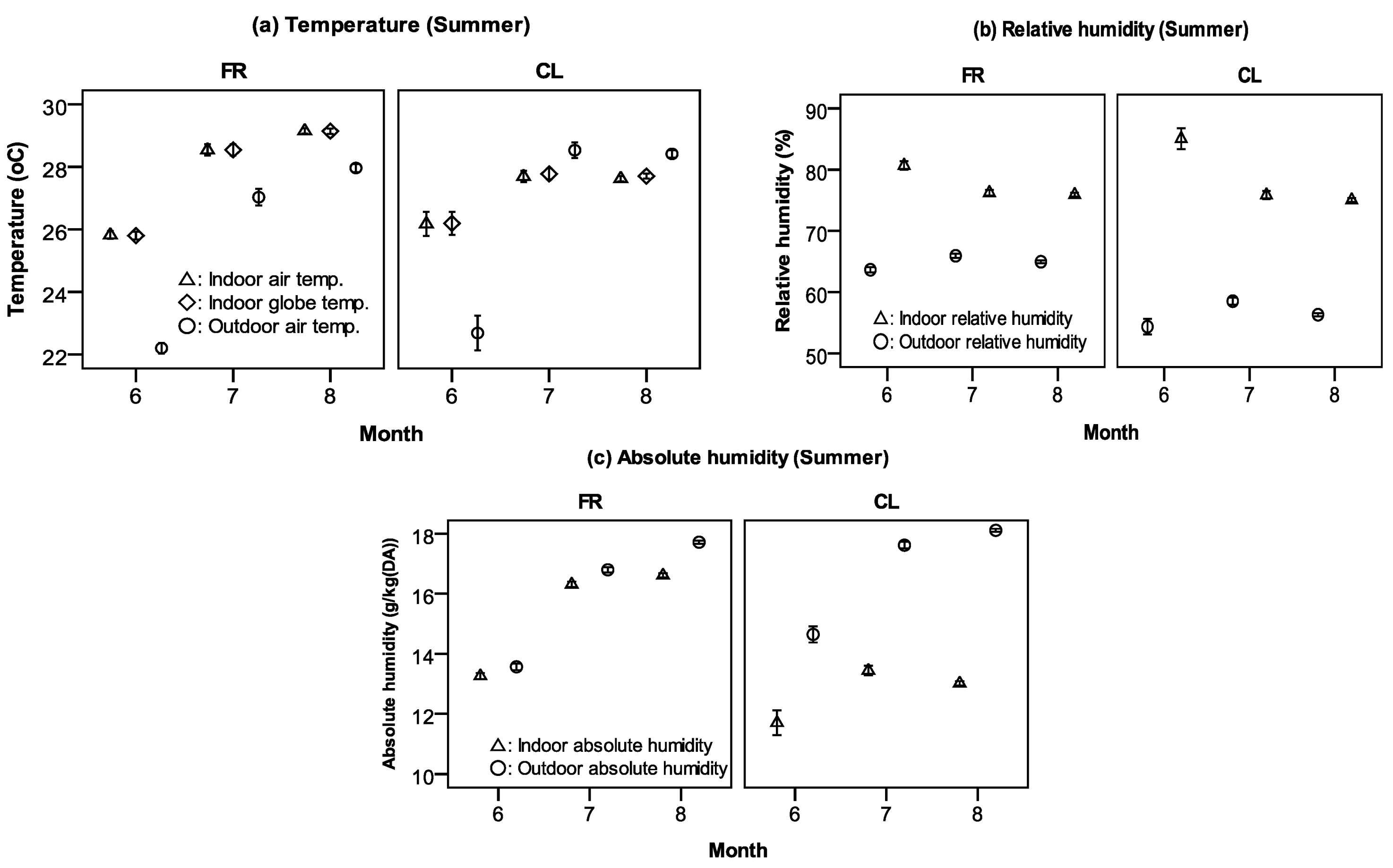
3.2. Distribution of Temperature and Humidity

The monthly mean indoor and globe temperature is very similar in FR and CL mode (Figure 2a), and the correlation coefficient is similarly high in both modes (Table 4). In FR mode, indoor temperatures are higher than the outdoor air temperature. However, in CL mode, the indoor temperatures are lower than the outdoor air temperature, except in June. The Japanese government recommends the indoor temperature settings of 28 °C in summer. The results showed that the mean indoor temperature setting in CL mode was similar to the recommendation. The mean indoor relative humidity and absolute humidity are lower than the outdoor relative humidities (Figure 2b,c). Due to the mechanical cooling, the mean indoor relative humidity or correlation coefficient of the CL mode is lower than the FR mode. The results showed that the relative humidity in FR mode is slightly higher than the standard: 60%. To predict the indoor air or globe temperature, regression analysis was conducted. The equations are given below.

FR mode:

T_i = 0.499T_o + 15.228 (n = 8280, R² = 0.59, S.E. = 0.005, p < 0.001)

(1)

T_g = 0.480T_o + 15.507 (n = 2785, R² = 0.58, S.E. = 0.008, p < 0.001)

(2)

CL mode:

T_i = 0.151T_o + 23.239 (n = 4860, R² = 0.04, S.E. = 0.10, p < 0.001)

(3)

T_g = 0.200T_o + 22.115 (n = 2109, R² = 0.10, S.E. = 0.013, p < 0.001)

(4)

T_i: indoor air temperature (°C); T_g: globe temperature (°C); T_o: outdoor air temperature (°C); n: number in sample; R²: coefficient of determination; S.E.: standard error of the regression coefficient; p: significance level of regression coefficient. The correlation between the indoor and outdoor temperature of the FR mode is higher than the CL mode (Figure 3).

Figure 2. Monthly mean values with 95% confidence interval (Error bar): (a) temperature; (b) relative humidity; (c) absolute humidity.

Figure 2. Monthly mean values with 95% confidence interval (Error bar): (a) temperature; (b) relative humidity; (c) absolute humidity.

Table 4. The correlation coefficient.

Mode	Items	Ti:To	Tg:To	Ti:Tg	RHi:RHo
FR	r	0.77	0.76	0.99	0.45
	N	8280	2785	2751	7924
CL	r	0.20	0.31	0.91	0.18
	N	4860	2109	1911	4856

Note: T_i: indoor air temperature (°C); T_g: indoor globe temperature (°C); T_o: outdoor air temperature (°C); RH_i: indoor relative humidity (%); RH_o: outdoor relative humidity (%); r: correlation coefficient; N: number in sample; correlation coefficient is significant at the 0.01 level (2-tailed).

Table 4. The correlation coefficient.

Mode	Items	Ti:To	Tg:To	Ti:Tg	RHi:RHo
FR	r	0.77	0.76	0.99	0.45
	N	8280	2785	2751	7924
CL	r	0.20	0.31	0.91	0.18
	N	4860	2109	1911	4856

Note: T_i: indoor air temperature (°C); T_g: indoor globe temperature (°C); T_o: outdoor air temperature (°C); RH_i: indoor relative humidity (%); RH_o: outdoor relative humidity (%); r: correlation coefficient; N: number in sample; correlation coefficient is significant at the 0.01 level (2-tailed).

Figure 3. Relation between the indoor and outdoor air temperature when voted (all raw data).

Figure 3. Relation between the indoor and outdoor air temperature when voted (all raw data).

3.3. Thermal Comfort

3.3.1. Comparison of the Scales

We wished to compare the performance of the SHASE scale and the ASHRAE scale. Table 5 shows the correlation of the thermal sensation and thermal preference with the room temperature. The SHASE scale is more strongly correlated with the thermal preference than is the ASHRAE scale. Also the SHASE scale correlates more strongly with the indoor air temperature and globe temperature. We have therefore chosen to use the SHASE scale rather than the ASHRAE scale for the analysis of the survey data.

Table 5. Correlation coefficient with ASHRAE and SHASE scales.

Mode	Items	ASHRAE			SHASE
		TP	Ti	Tg	TP	Ti	Tg
FR	r	0.74	0.47	0.42	0.82	0.49	0.47
	N	5540	5451	2789	7526	8282	2788
CL	r	0.70	0.26	0.26	0.81	0.28	0.31
	N	3859	3588	2109	4800	4857	2109

Note: TP: thermal preference; T_i: indoor air temperature (°C); T_g: globe temperature (°C); p < 0.001; p: significance level; r: correlation coefficient; N: number of sample.

Table 5. Correlation coefficient with ASHRAE and SHASE scales.

Mode	Items	ASHRAE			SHASE
		TP	Ti	Tg	TP	Ti	Tg
FR	r	0.74	0.47	0.42	0.82	0.49	0.47
	N	5540	5451	2789	7526	8282	2788
CL	r	0.70	0.26	0.26	0.81	0.28	0.31
	N	3859	3588	2109	4800	4857	2109

Note: TP: thermal preference; T_i: indoor air temperature (°C); T_g: globe temperature (°C); p < 0.001; p: significance level; r: correlation coefficient; N: number of sample.

3.3.2. Distribution of Thermal Sensation

Table 6 shows the percentages of the thermal sensations in each scale category for the FR and CL modes. The mean thermal sensation was 4.7 in FR mode, 4.2 in CL mode. Even when residents used the cooling, they sometimes felt “hot”. The proportion of people voting in the thermal comfort zone (votes 3, 4 or 5) in the FR and CL modes is 83% and 94% (Table 6). It can be said that residents were generally satisfied with the thermal environment of their houses. This may be because the residents are well-adapted to the local climate and culture.

Table 6. Percentage of thermal sensation on the SHASE scale in FR and CL modes.

Mode	Items	Thermal Sensation							Total
		1	2	3	4	5	6	7
FR	N	2	8	210	4044	2701	1,173	257	8395
	P (%)	0.0	0.1	2.5	48.2	32.2	14.0	3.1	100
CL	N	6	30	368	3487	964	226	49	5130
	P (%)	0.1	0.6	7.2	68.0	18.8	4.4	1.0	100

Note: N: number of sample; P: percentage.

Table 6. Percentage of thermal sensation on the SHASE scale in FR and CL modes.

Mode	Items	Thermal Sensation							Total
		1	2	3	4	5	6	7
FR	N	2	8	210	4044	2701	1,173	257	8395
	P (%)	0.0	0.1	2.5	48.2	32.2	14.0	3.1	100
CL	N	6	30	368	3487	964	226	49	5130
	P (%)	0.1	0.6	7.2	68.0	18.8	4.4	1.0	100

Note: N: number of sample; P: percentage.

To locate the thermal comfort zone, Probit regression analysis [21] was conducted for the thermal sensation vote (TSV) categories and the temperature, for FR and CL modes. The analysis method is Ordinal regression using Probit as the link function and the temperature as the covariate.

The results of the Probit analysis is shown in Table 7. The temperature corresponding to the median response (Probit = 0) is calculated by dividing the constant by regression coefficient. For example, the mean temperature of the first equation will be 4.151/0.288 = 14.4 °C (Table 7). The inverse of the Probit regression coefficient is the standard deviation of the cumulative Normal distribution. For example, the standard deviation of air temperature of the FR mode will be 1/0.288 = 3.472 °C (Table 7). These calculations are fully given in the Table 7. Transforming the Probits using the following function into proportions gives the curve of Figure 4a–d. The vertical axis is the proportion of votes.

Probability = CDF.NORMAL (quant, mean, S.D.)

(5)

where “CDF.NORMAL” is the Cumulative Distribution Function for the normal distribution, “quant” is the indoor air temperature (°C) or globe temperature (°C); the “mean” and “S.D.” are given in the Table 7.

Figure 4. Proportion of thermal sensation vote (TSV) or comfortable (TSV 3, 4 or 5) for temperatures: (a) and (b) FR mode; (c) and (d) CL mode; (e) and (f) FR and CL modes.

Figure 4. Proportion of thermal sensation vote (TSV) or comfortable (TSV 3, 4 or 5) for temperatures: (a) and (b) FR mode; (c) and (d) CL mode; (e) and (f) FR and CL modes.

Table 7. Percentage of thermal sensation in FR and CL modes.

Mode	Indoor Air Temperature Ti (°C)						Globe Temperature Tg (°C)
	Equation *	Mean	S.D.	N	R2	S.E.	Equation *	Mean	S.D.	N	R2	S.E.
FR	P(≤1) = 0.288Ti − 4.151	14.4	3.472	8282	0.25	0.006	P(≤1) = 0.274Tg − 3.784	13.8	3.650	2788	0.23	0.011
	P(≤2) = 0.288Ti − 4.602	16.0					P(≤2) = 0.274Tg − 4.156	15.2
	P(≤3) = 0.288Ti − 5.843	20.3					P(≤3) = 0.274Tg − 5.282	19.3
	P(≤4) = 0.288Ti − 8.186	28.4					P(≤4) = 0.274Tg − 7.851	28.7
	P(≤5) = 0.288Ti − 9.299	32.3					P(≤5) = 0.274Tg − 8.999	32.8
	P(≤6) = 0.288Ti − 10.376	36.0					P(≤6) = 0.274Tg − 10.002	36.5
CL	P(≤1) = 0.180Ti − 1.821	10.1	5.556	4857	0.08	0.009	P(≤1) = 0.228Tg − 2.895	12.7	4.386	2109	0.09	0.016
	P(≤2) = 0.180Ti − 2.394	13.3					P(≤2) = 0.228Tg − 3.538	15.5
	P(≤3) = 0.180Ti − 3.483	19.4					P(≤3) = 0.228Tg − 4.750	20.8
	P(≤4) = 0.180Ti − 5.765	32.0					P(≤4) = 0.228Tg − 6.917	30.3
	P(≤5) = 0.180Ti − 6.648	36.9					P(≤5) = 0.228Tg − 8.244	36.2
	P(≤6) = 0.180Ti − 7.422	41.2					P(≤6) = 0.228Tg − 9.190	40.3

Note: P_(≤1) is the probit of proportion of the votes that are 1 and less, P_(≤2) is the probit of the proportion that are 2 and less, and so on; S.D.: standard deviation of the cumulative normal distribution; N: number of sample; R²: cox and snell R²; S.E.: standard error of the regression coefficient; * regression coefficient is significant (p < 0.001).

Table 7. Percentage of thermal sensation in FR and CL modes.

Mode	Indoor Air Temperature Ti (°C)						Globe Temperature Tg (°C)
	Equation *	Mean	S.D.	N	R2	S.E.	Equation *	Mean	S.D.	N	R2	S.E.
FR	P(≤1) = 0.288Ti − 4.151	14.4	3.472	8282	0.25	0.006	P(≤1) = 0.274Tg − 3.784	13.8	3.650	2788	0.23	0.011
	P(≤2) = 0.288Ti − 4.602	16.0					P(≤2) = 0.274Tg − 4.156	15.2
	P(≤3) = 0.288Ti − 5.843	20.3					P(≤3) = 0.274Tg − 5.282	19.3
	P(≤4) = 0.288Ti − 8.186	28.4					P(≤4) = 0.274Tg − 7.851	28.7
	P(≤5) = 0.288Ti − 9.299	32.3					P(≤5) = 0.274Tg − 8.999	32.8
	P(≤6) = 0.288Ti − 10.376	36.0					P(≤6) = 0.274Tg − 10.002	36.5
CL	P(≤1) = 0.180Ti − 1.821	10.1	5.556	4857	0.08	0.009	P(≤1) = 0.228Tg − 2.895	12.7	4.386	2109	0.09	0.016
	P(≤2) = 0.180Ti − 2.394	13.3					P(≤2) = 0.228Tg − 3.538	15.5
	P(≤3) = 0.180Ti − 3.483	19.4					P(≤3) = 0.228Tg − 4.750	20.8
	P(≤4) = 0.180Ti − 5.765	32.0					P(≤4) = 0.228Tg − 6.917	30.3
	P(≤5) = 0.180Ti − 6.648	36.9					P(≤5) = 0.228Tg − 8.244	36.2
	P(≤6) = 0.180Ti − 7.422	41.2					P(≤6) = 0.228Tg − 9.190	40.3

Note: P_(≤1) is the probit of proportion of the votes that are 1 and less, P_(≤2) is the probit of the proportion that are 2 and less, and so on; S.D.: standard deviation of the cumulative normal distribution; N: number of sample; R²: cox and snell R²; S.E.: standard error of the regression coefficient; * regression coefficient is significant (p < 0.001).

The highest line is for category 1 (very cold) and so on successively. Thus, it can be seen that the temperature for thermal neutrality (a probability of 0.5) is around 24 to 26 °C.

Reckoning the three central categories as representing thermal comfort, and transforming the Probits into proportions gives the bell-curve of Figure 4e,f. The result is remarkable in two respects. The proportion of people comfortable at the optimum is very high, only just less that 100%, and the range over which 80% are comfortable is wide—from around 18 to 32 °C. This is presumably because people in their own homes are free to clothe themselves according to the room temperature, without the constraints that are apt to apply at the office.

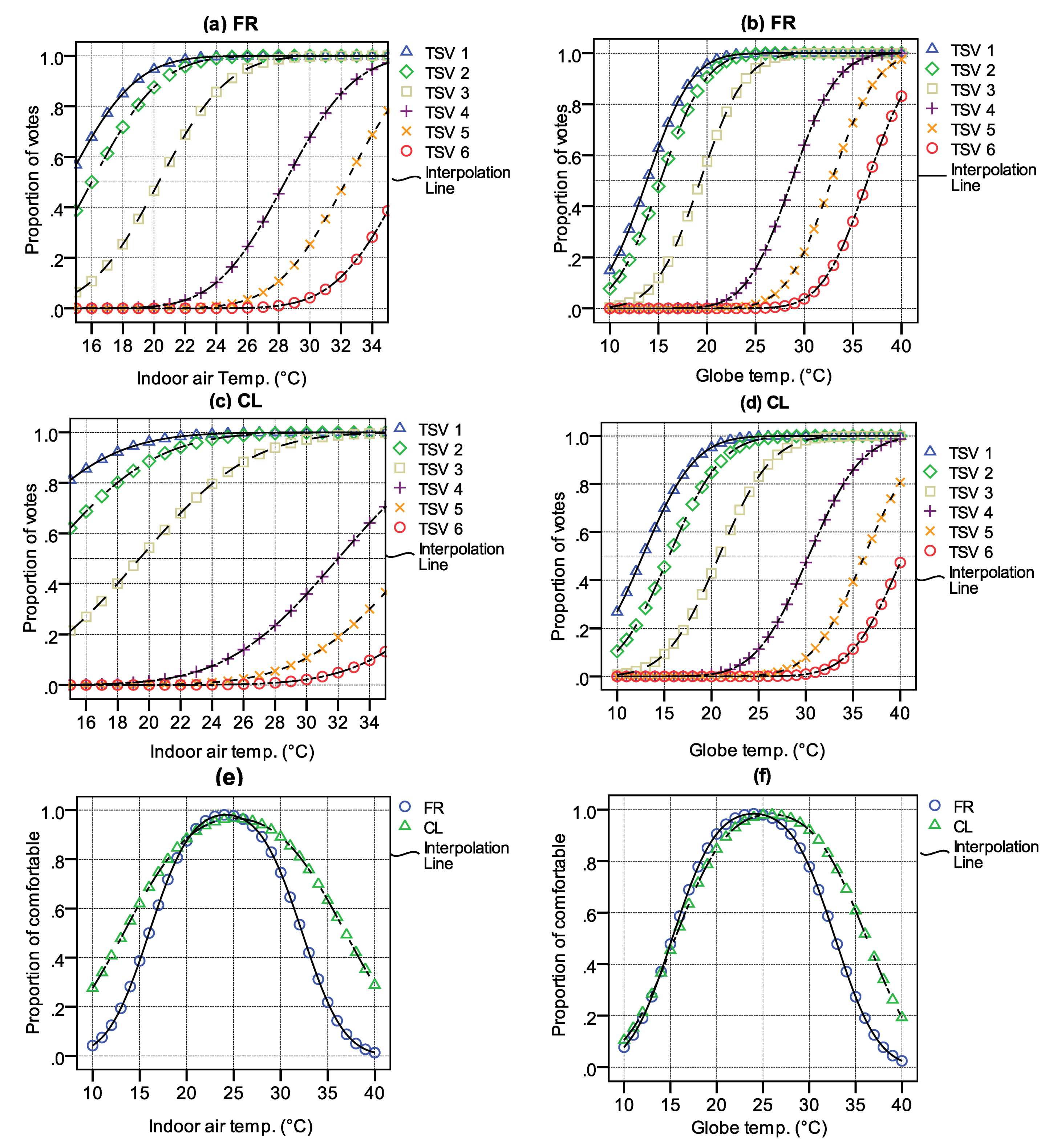
3.4. The Comfort Temperature

To predict the comfort temperature, regression analysis of the thermal sensation and indoor air or globe temperature was conducted (Figure 5). The following regression equations are obtained.

FR mode:

C = 0.187T_i − 0.637 (n = 8282, R² = 0.24, S.E. = 0.004, p < 0.001)

(6)

C = 0.164T_g − 0.004 (n = 2788, R² = 0.22, S.E. = 0.006, p < 0.001)

(7)

CL mode:

C = 0.106T_i + 1.294 (n = 4857, R² = 0.08, S.E. = 0.005, p < 0.001)

(8)

C = 0.124T_g + 0.829 (n = 2109, R² = 0.09, S.E. = 0.008, p < 0.001)

(9)

C is the thermal sensation vote.

Figure 5. Relation between thermal sensation and the temperature: (a) Thermal sensation and indoor air temperature; (b) Thermal sensation and indoor globe temperature.

Figure 5. Relation between thermal sensation and the temperature: (a) Thermal sensation and indoor air temperature; (b) Thermal sensation and indoor globe temperature.

The regression coefficient for the FR mode is higher than that of the CL. When the indoor or globe comfort temperature is predicted by substituting 4 (neutral) for C in the Equations (6) to (9), this gives T_i = 24.8 °C or T_g = 24.4 °C in the FR mode and T_i = 25.5 °C or T_g = 25.6 °C in the CL mode.

The presence of behavioral adaptation in the data renders the evaluation of comfort temperatures suspect, tending to artificially lower the regression coefficients and therefore the estimates of the comfort temperature. There is therefore a problem in applying the regression method in the presence of adaptive behavior, as has been found in previous research [2,7]. So to avoid this problem the comfort temperatures have been re-estimated using the Griffiths method (in the next section).3.4.2. Griffiths Method

Griffiths [22] suggested a way in which the comfort temperature can be calculated from a small sample of data. Griffiths made the assumption that the increase in temperature for each scale point on the thermal sensation scale was effectively 3 °C for a seven point scale [23]. This means that for each thermal sensation vote away from neutral, he subtracted or added 3 °C from the actual temperature at the time to obtain the temperature that might be expected to result in neutrality [23]. The detail of the Griffiths method can be found in the various publications [9,23,24]. The comfort temperature is predicted by the Griffiths’ method which is given below.

T_c = T + (4 − C)/a

(10)

where T_c is the comfort temperature by Griffiths’ method (°C), T is the indoor air temperature (°C) or globe temperature (°C) and a is the regression coefficient.

In applying the Griffiths’ method, Nicol et al. [9] and Humphreys et al. [25] used the constants 0.25, 0.33 and 0.50 for a 7 point thermal sensation scale. We have also investigated the comfort temperature using these regression coefficients. The mean comfort temperature with each coefficient is not very different (Table 8), so it matters little which coefficient is adopted. The comfort temperature calculated using a coefficient of 0.50 is used for further analysis.

Table 8. Comfort temperature predicted by Griffiths’ method.

Mode	RC	Tci (°C)			Tcg (°C)
		N	Mean	S.D.	N	Mean	S.D.
FR	0.25	8282	25.7	3.1	2788	25.7	3.0
	0.33	8282	26.3	2.5	2788	26.2	2.5
	0.50	8282	27.0	2.1	2788	26.8	2.1
CL	0.25	4857	26.7	2.9	2109	26.7	2.7
	0.33	4857	26.9	2.4	2109	27.0	2.2
	0.50	4857	27.1	2.0	2109	27.2	1.8

Note: RC: regression coefficient; T_ci: comfort indoor air temperature; T_cg: comfort globe temperature; N: number of sample; S.D.: standard deviation.

Table 8. Comfort temperature predicted by Griffiths’ method.

Mode	RC	Tci (°C)			Tcg (°C)
		N	Mean	S.D.	N	Mean	S.D.
FR	0.25	8282	25.7	3.1	2788	25.7	3.0
	0.33	8282	26.3	2.5	2788	26.2	2.5
	0.50	8282	27.0	2.1	2788	26.8	2.1
CL	0.25	4857	26.7	2.9	2109	26.7	2.7
	0.33	4857	26.9	2.4	2109	27.0	2.2
	0.50	4857	27.1	2.0	2109	27.2	1.8

Note: RC: regression coefficient; T_ci: comfort indoor air temperature; T_cg: comfort globe temperature; N: number of sample; S.D.: standard deviation.

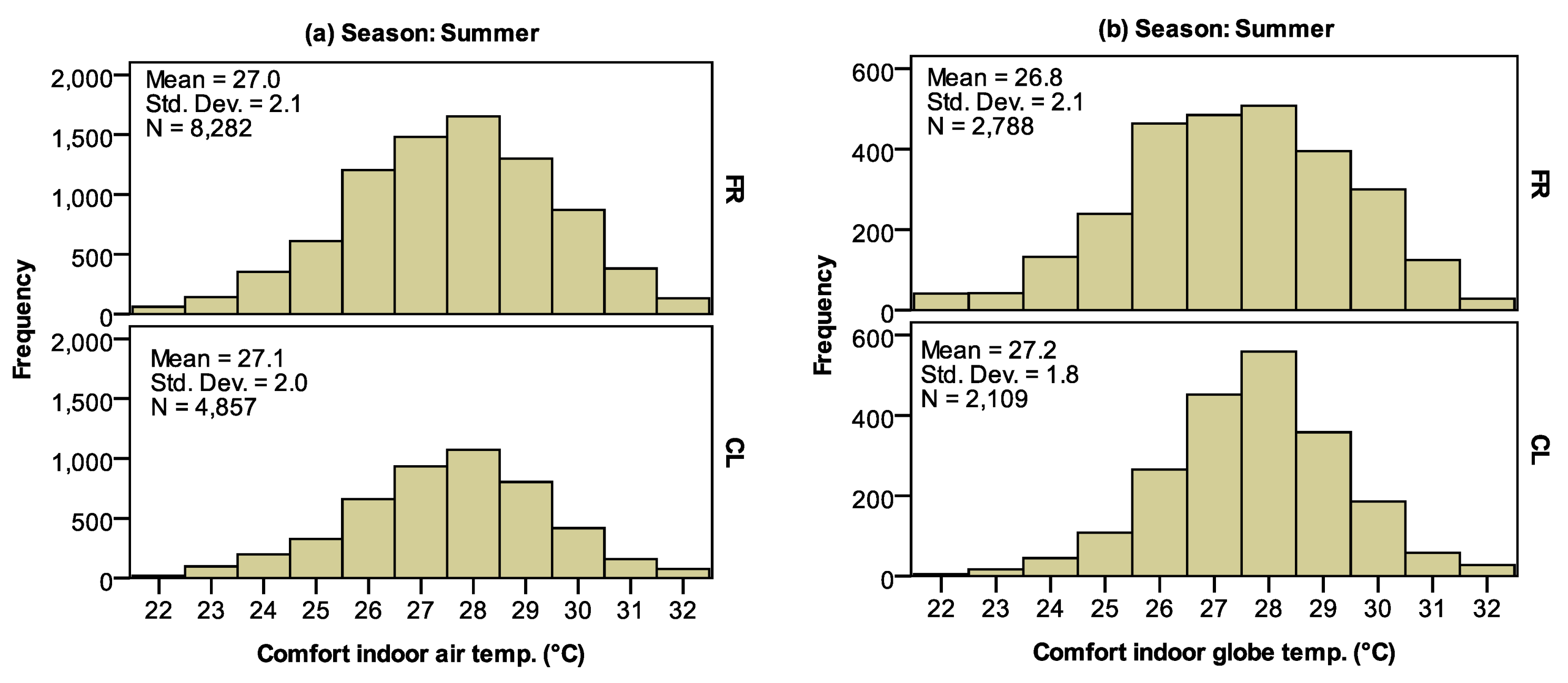
The mean comfort indoor air or globe temperature by the Griffiths’ method is 27.0 °C or 26.8 °C in FR mode and 27.1 °C or 27.2 °C in CL mode (Figure 6). The use of the Griffiths method brings together the neutral (comfort) temperatures for the air temperature and the globe temperature, again suggesting that it is more valid than the simple regression model.

Table 9 shows a comparison of the comfort temperature obtained in this study with existing research. The comfort temperature of the existing research is similar to this research.

Figure 6. Comfort temperature predicted by Griffiths method: (a) Comfort indoor air temperature; (b) Comfort globe temperature.

Figure 6. Comfort temperature predicted by Griffiths method: (a) Comfort indoor air temperature; (b) Comfort globe temperature.

Table 9. Comparison of comfort temperature in summer with existing research.

Area	References	Tempeature for Tc (°C)	Comfort Tempeature Tc (°C)
Japan (Kanto)	This study (FR mode)	Tg	26.8
Japan (Gifu)	Rijal et al. [2]	Ti	26.1
Japan (Kansai)	Nakaya et al. [1]	Top	27.6
China	Han et al. [3]	Top	28.6
Singapore	de Dear et al. [4]	Top	28.5
Malaysia	Djamila et al. [5]	Ti	30.1
Indonesia	Fedriadi and Wong [6]	Top	29.2
Nepal	Rijal et al. [7]	Tg	21.1–30.0
India	Indraganti [8]	Tg	29.2
Pakistan	Nicol and Roaf [10]	Tg	26.7–29.9
Iran	Heidari & Sharples [11]	Ti	28.4
UK	Rijal and Stevenson [12]	Ti	22.9

Note: T_g: globe temperature. (°C), T_i: indoor air temperature. (°C), T_op: operative temperature. (°C).

Table 9. Comparison of comfort temperature in summer with existing research.

Area	References	Tempeature for Tc (°C)	Comfort Tempeature Tc (°C)
Japan (Kanto)	This study (FR mode)	Tg	26.8
Japan (Gifu)	Rijal et al. [2]	Ti	26.1
Japan (Kansai)	Nakaya et al. [1]	Top	27.6
China	Han et al. [3]	Top	28.6
Singapore	de Dear et al. [4]	Top	28.5
Malaysia	Djamila et al. [5]	Ti	30.1
Indonesia	Fedriadi and Wong [6]	Top	29.2
Nepal	Rijal et al. [7]	Tg	21.1–30.0
India	Indraganti [8]	Tg	29.2
Pakistan	Nicol and Roaf [10]	Tg	26.7–29.9
Iran	Heidari & Sharples [11]	Ti	28.4
UK	Rijal and Stevenson [12]	Ti	22.9

Note: T_g: globe temperature. (°C), T_i: indoor air temperature. (°C), T_op: operative temperature. (°C).

3.5. Comfort Temperature and Humidity

The humidity is important in the hottest season. In a moist environment, it has been observed that people become uncomfortable with a smaller change in temperature than they do in a dry environment [15]. To explore a possible effect of humidity, the comfort temperature is analyzed by relating it to the relative humidity, absolute humidity and skin moisture. The comfort temperatures were correlated with the indoor relative humidity, absolute humidity and skin moisture sensation (Table 10). However, the correlation effect of the comfort temperature and relative humidity might have simply been attributable to the correlation between air temperature and relative humidity. So to further investigate the effect of humidity on the comfort temperature, multiple regression analysis was conducted for the FR mode.

T_ci = 0.623T_i − 0.006RH_i + 9.8

(11)

(n = 8282, R² = 0.47, S.E.₁ = 0.007, S.E.₂ = 0.002, p₁ < 0.001, p₂ = 0.001)

T_ci = 0.656T_i − 0.039AH_i + 9.0

(12)

(n = 8282, R² = 0.47, S.E.₁ = 0.010, S.E.₂ = 0.008, p₁ and p₂ < 0.001)

T_ci = 0.825T_i − 1.317SM + 5.8

(13)

(n = 7868, R² = 0.68, S.E.₁ = 0.006, S.E.₂ = 0.019, p₁ and p₂ < 0.001).

where T_ci: Comfort indoor air temperature (°C); RH_i: Indoor relative humidity (%); AH_i: Indoor absolute humidity (g/kg (Dry Air)); SM: Skin moisture sensation; S.E.₁ and S.E.₂: Standard Error of regression coefficient for first and second terms; p₁ and p₂: Significance level of the regression coefficients of the first and second terms.

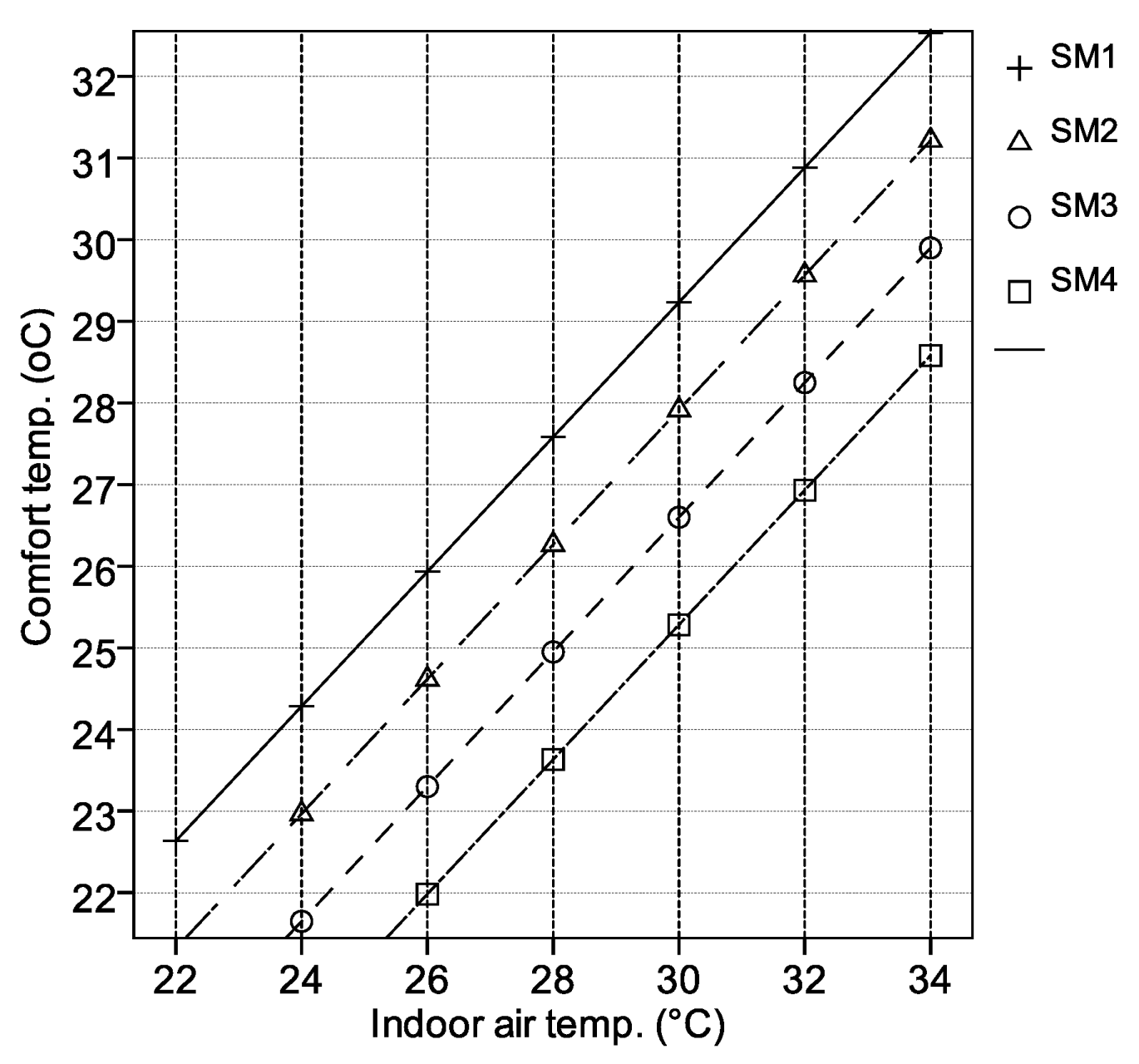
As may be seen from the equations, neither the relative humidity nor the absolute humidity had, in these data, an important effect on the comfort temperature. However, Nicol [15] found that in a humid climate or in conditions when the relative humidity is high people may require temperatures that are about 1°C lower to remain comfortable. As for the skin moisture, Equation (13) shows it has a considerable effect on the comfort temperature, an increase of one category in the level of skin moisture reducing the comfort temperature by approximately 1.3 K (Figure 7).

Table 10. Correlation coefficient in FR mode.

Items	Tci:RHi	Tcg:RHi	Tci:AHi	Tcg:AHi	Tci:SM	Tcg:SM
r	−0.10	−0.15	0.42	0.38	−0.11	−0.06
p	<0.001	<0.001	<0.001	<0.001	<0.001	0.003
N	8282	2750	8282	2750	7868	2786

Note: r: Correlation coefficient; p: Significance level; N: Number of sample; T_ci: Comfort indoor temperature (°C); T_cg: Comfort globe temperature (°C); RH_i: Indoor relative humidity (%); AH_i: Indoor absolute humidity (g/kg(Dry Air)); SM: Skin moisture sensation.

Table 10. Correlation coefficient in FR mode.

Items	Tci:RHi	Tcg:RHi	Tci:AHi	Tcg:AHi	Tci:SM	Tcg:SM
r	−0.10	−0.15	0.42	0.38	−0.11	−0.06
p	<0.001	<0.001	<0.001	<0.001	<0.001	0.003
N	8282	2750	8282	2750	7868	2786

Note: r: Correlation coefficient; p: Significance level; N: Number of sample; T_ci: Comfort indoor temperature (°C); T_cg: Comfort globe temperature (°C); RH_i: Indoor relative humidity (%); AH_i: Indoor absolute humidity (g/kg(Dry Air)); SM: Skin moisture sensation.

Figure 7. Relation between the comfort temperature and the indoor air temperature for the four levels of skin moisture.

Figure 7. Relation between the comfort temperature and the indoor air temperature for the four levels of skin moisture.

Nicol [26] found that when indoor air temperature is 31–40 °C, increased air speed reduced the assessed skin moisture. Our results therefore imply that the evaporation of the skin moisture is important in raising the comfort temperature in Japan’s hot and humid season.

3.6. A Comparison with the Adaptive Model

It is well known that people adapt to the temperature of their accommodation, and thus comfort temperature has corresponding seasonal and regional differences in relation to the outdoor temperature [20]. To predict such indoor comfort temperatures, the CEN and Chartered Institution of Building Services Engineers (CIBSE) proposed an adaptive model for office buildings. We compare our results with these adaptive models.

The running mean outdoor temperature (T_rm) is used in the adaptive model. It is the exponentially weighted daily mean outdoor temperature. It is calculated using the following equation [14,23,27,28].

T_rm = αT_rm−1 + (1 − α)T_od−1

(14)

where T_rm−1 is the running mean outdoor temperature for the previous day (°C), T_od−1 is the daily mean outdoor temperature for the previous day (°C). So, if the running mean has been calculated (or assumed) for one day, then it can be readily calculated for the next day, and so on. α is a constant between the 0 and 1 which defines the speed at which the running mean responds to the outdoor air temperature. In this research α is assumed to be 0.8, a value previously found to be appropriate.

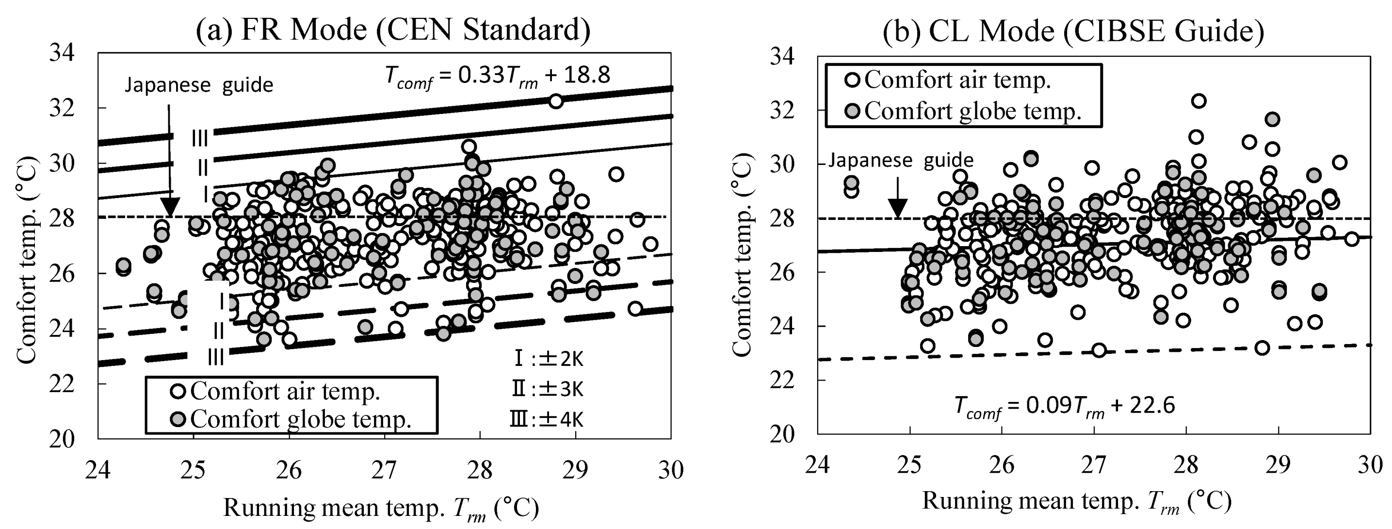
Figure 8 shows the relation between the comfort temperature and the running mean outdoor temperature. The six parallel lines in Figure 8a show the acceptable zone of the adaptive model of CEN standard [14]. The two parallel lines in Figure 8b show upper and lower margins of the comfort temperature [28]. The Japanese guide line is also shown in the figure.

Generally the comfort temperature of FR mode is within the acceptable zone of the adaptive model. As for the CL mode, the comfort temperature is higher than the CIBSE guide [28] and Japanese guide line. The results showed that the residents are adapting to the higher indoor air temperature of the houses.

Figure 8. Comparison with the adaptive model: (a) FR mode (CEN standard); (b) CL mode (CIBSE guide). Each point represents the monthly mean comfort temperature of each subject.

Figure 8. Comparison with the adaptive model: (a) FR mode (CEN standard); (b) CL mode (CIBSE guide). Each point represents the monthly mean comfort temperature of each subject.

3.7. Occupant Behaviour

As we have shown in the previous sections, the residents questioned are adapting in summertime to higher indoor air temperature of the houses. Residents might be regulating their thermal comfort by using various adaptations: behavioral, physiological and psychological [29]. This section focuses on behavioral adaptation. Nicol and Humphreys [30] made use of logistic regression analysis to predict occupant control behavior in naturally ventilated buildings. We have also adopted the logistic regression method to predict the window opening and fan use in the living room. The relationship between the probability of windows being open or a fan in use (p) and the indoor or outdoor temperature (T) is of the form:

logit(p) = log [p/(1 − p)] = bT + c

(15)

p = exp^{(bT + c)}/[1 + exp^{(bT + c)}]

(16)

where exp(exponential function) is the base of natural logarithm, b is the regression coefficient for T, and c is the constant in the regression equation.

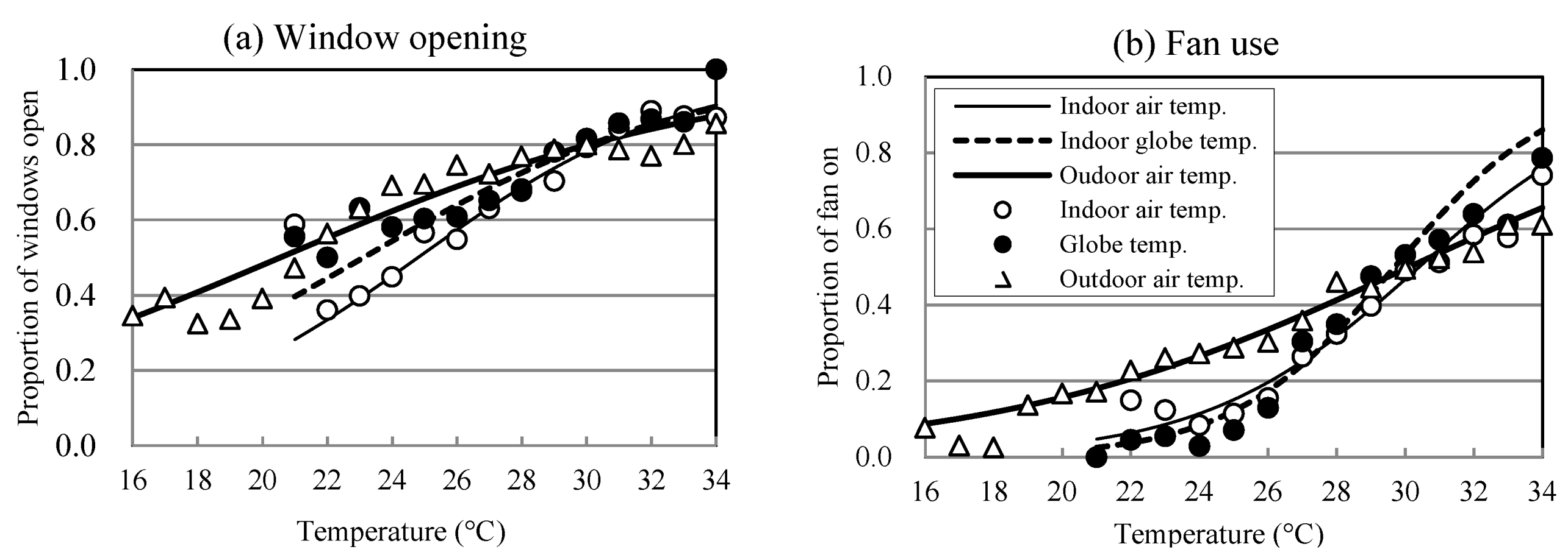
The following regression equations were obtained in between the window opening or fan use and temperatures for FR mode.

Window opening:

logit(p) = 0.246T_i – 6.1 (n = 8216, R² = 0.06, S.E. = 0.011, p < 0.001)

(17)

logit(p) = 0.199T_g − 4.6 (n = 2771, R² = 0.04, S.E. = 0.019, p < 0.001)

(18)

logit(p) = 0.146T_o – 3.0 (n = 8254, R² = 0.05, S.E. = 0.007, p < 0.001)

(19)

Fan use:

logit(p) = 0.319T_i − 9.7 (n = 7961, R² = 0.09, S.E. = 0.013, p < 0.001)

(20)

logit(p) = 0.421T_g – 12.5 (n = 2749, R² = 0.15, S.E. = 0.023, p < 0.001)

(21)

logit(p) = 0.166T_o − 5.0 (n = 7993, R² = 0.06, S.E. = 0.008, p < 0.001)

(22)

where T_i is indoor air temperature (°C), T_g is indoor globe temperature (°C), T_o is outdoor air temperature (°C) and R² is Cox and Snell R².

Even though the coefficient of determination is low, the equations are statistically significant. These equations are shown in Figure 9. The predicted proportion of window opening or fan use is well matched with the measured values, as can be seen from the figure (the points shown are the proportions for the data in groups of width 1 K). The proportion of window opening or fan use is increased when temperature rises. The window opening behavior is similar to that found in previous research [2,24].

The regression coefficient for indoor air temperature or globe temperature is higher than the outdoor air temperature. It seems that the occupants respond more closely to the indoor temperatures than outdoor air temperature while operating the windows and fans.

Window opening and fan use might be important to increase the air movement and modify the indoor air temperature. Window opening is effective at increasing the indoor comfort temperature [2,31]. Theoretically, if wind velocity is 1 m/s, the indoor comfort temperature can be increased by some 3 or 4 °C [15,32,33]. Nicol [15] found that the presence of air movement can be equivalent to a reduction in indoor temperature of as much as 4 °C. When outdoor running mean temperature is 30 °C, the indoor comfort temperature when the fan is on is 31 °C which is 2.2 °C higher than when the fan is off [24,33].

Thus, the results showed that residents undertake behavioral adaptation to regulate their hot and humid thermal environment.

Figure 9. Relation between the use of controls and temperature: (a) Window opening; (b) Fan use. Measured values were grouped for every 1 °C for temperatures. The grouped data for samples less than 10 are not shown.

Figure 9. Relation between the use of controls and temperature: (a) Window opening; (b) Fan use. Measured values were grouped for every 1 °C for temperatures. The grouped data for samples less than 10 are not shown.

4. Conclusions

In order to explore the variation of the comfort temperature, and to investigate the behavioral adaptation in Japanese houses, we conducted a thermal comfort and occupant behavior survey in 120 houses in living-rooms and bedrooms for the hot and humid season in the Kanto region of Japan. The chief findings were as follows:

• The proportion of people in thermal comfort was 83% in FR mode, showing that the residents were generally well-adapted and satisfied with the thermal environment in their houses.
• The mean comfort temperature in free running mode was 27.0 °C in hot and humid season. The comfort temperature obtained in this study is within the acceptable zone of the CEN adaptive model.
• The comfort temperature was related to the skin moisture sensation, and thus the evaporation of the skin moisture raises the comfort temperature in the hot and humid season.
• The residents adapted to hot and humid environments by increasing the air movement usage through actions such as opening the windows and using fans. The design of the openable window and ceiling fan are important for the success of adaptive thermal comfort in a hot and humid climate.

The results show what room temperatures were prevalent in this large sample of Japanese dwellings during the summer. That the residents were largely happy with these conditions indicates that the dwellings were of suitable design for the climate and culture. It is of course unwise to generalize from these results to dwellings worldwide. However, that our results are similar to those found from surveys in dwellings in other countries with hot and humid summers, and that our results are consistent with those portrayed by the European adaptive standard, suggest a wider range of applicability.

References

1. Nakaya, T.; Matsubara, N.; Kurazumi, Y. A field study of thermal environment and thermal comfort in Kansai region, Japan: Neutral temperature and acceptable range in summer. J. Environ. Eng. AIJ 2005, 597, 51–56. [Google Scholar]
2. Rijal, H.B.; Honjo, M.; Kobayashi, R.; Nakaya, T. Investigation of comfort temperature, adaptive model and the window opening behaviour in Japanese houses. Archit. Sci. Rev. 2013, 56, 54–69. [Google Scholar] [CrossRef]
3. Han, J.; Zhang, G.; Zhang, Q.; Zhang, J.; Liu, J.; Tian, L.; Zheng, C.; Hao, J.; Lin, J.; Liu, Y.; et al. Field study on occupants’ thermal comfort and residential thermal environment in a hot-humid climate of China. Build. Environ. 2007, 42, 4043–4050. [Google Scholar] [CrossRef]
4. De Dear, R.J.; Leow, K.G.; Foo, S.C. Thermal comfort in the humid tropics: Field experiments in air-conditioned and naturally ventilated buildings in Singapore. Int. J. Biometeorol. 1991, 34, 259–265. [Google Scholar] [CrossRef]
5. Djamila, H.; Chu, C.M.; Kumaresan, S. Field study of thermal comfort in residential buildings in the equatorial hot-humid climate of Malaysia. Build. Environ. 2013, 62, 133–142. [Google Scholar] [CrossRef]
6. Feriadi, H.; Wong, N.H. Thermal comfort for naturally ventilated houses in Indonesia. Energy Build. 2004, 36, 614–626. [Google Scholar] [CrossRef]
7. Rijal, H.B.; Yoshida, H.; Umemiya, N. Seasonal and regional differences in neutral temperatures in Nepalese traditional vernacular houses. Build. Environ. 2010, 45, 2743–2753. [Google Scholar] [CrossRef]
8. Indraganti, M. Using the adaptive model of thermal comfort for obtaining the indoor neutral temperature: Findings form a field study in Hyderabad. Build. Environ. 2010, 45, 519–536. [Google Scholar] [CrossRef]
9. Nicol, F.; Jamy, G.N.; Sykes, O.; Humphreys, M.; Roaf, S.; Hancock, M. A Survey of Thermal Comfort in Pakistan toward New Indoor Temperature Standards; Oxford Brookes University: Oxford, UK, 1994. [Google Scholar]
10. Nicol, F.; Roaf, S. Pioneering new indoor temperature standards: The Pakistan project. Energy Build. 1996, 23, 169–174. [Google Scholar] [CrossRef]
11. Heidari, S.; Sharples, S. A comparative analysis of short-term and long-term thermal comfort surveys in Iran. Energy Build. 2002, 34, 607–614. [Google Scholar] [CrossRef]
12. Rijal, H.B.; Stevenson, F. Thermal Comfort in UK Housing to Avoid Overheating: Lessons from a “Zero Carbon” Case Study. In Proceedings of the Conference Adapting to Change: New Thinking on Comfort, Windsor, UK, 9–11 April 2010.