Optimizing Whole House Deep Energy Retrofit Packages: A Case Study of Existing Chicago-Area Homes

Abstract

Improving the energy efficiency of the residential building stock plays a key role in mitigating global climate change. New guidelines are targeting widespread application of deep energy retrofits to existing homes that reduce their annual energy use by 50%, but questions remain as to how to identify and prioritize the most cost-effective retrofit measures. This work demonstrates the utility of whole building energy simulation and optimization software to construct a “tool-box” of prescriptive deep energy retrofits that can be applied to large portions of the existing housing stock. We consider 10 generally representative typology groups of existing single-family detached homes built prior to 1978 in the Chicago area for identifying cost-optimal deep energy retrofit packages. Simulations were conducted in BEopt and EnergyPlus operating on a cloud-computing platform to first identify cost-optimal enclosure retrofits and then identify cost-optimal upgrades to heating, ventilation, and air-conditioning (HVAC) systems. Results reveal that prescriptive retrofit packages achieving at least 50% site energy savings can be defined for most homes through a combination of envelope retrofits, lighting upgrades, and upgrades to existing HVAC system efficiency or conversion to mini-split heat pumps. The average upfront cost of retrofits is estimated to be ~$14,400, resulting in average annual site energy savings of ~54% and an average simple payback period of ~25 years. Widespread application of these prescriptive retrofit packages across the existing Chicago-area residential building stock is predicted to reduce annual site energy use by 3.7 × 10¹⁶ J and yield approximately $280 million USD in annual energy savings.

1. Introduction

Improving the energy efficiency of the building stock plays a key role in mitigating global climate change [1]. Importantly in the U.S., residential buildings are responsible for over 20% of primary energy consumption [2] and greenhouse gas emissions [3]. The vast majority of this share is associated with detached single-family dwellings, which make up approximately 70% of the existing residential building stock [4]. Correspondingly, several governmental and non-governmental organizations have proposed aggressive targets for applying deep energy retrofits to achieve a minimum of 50% reductions in annual energy use by existing residential buildings [5,6]. These goals create both a challenge and an opportunity for older homes in the U.S. and abroad.

There are a number of approaches commonly used to select and apply energy efficiency retrofits to buildings. In practice, it is common to apply a package, or “tool-box,” of prescriptive deep energy retrofits [7,8,9,10,11]. This approach has the advantage of reducing the time and effort required for energy analysis on individual homes while allowing for efficient training of contractors to apply the same, or similar, retrofits to a large number of homes in a systematic way. However, prescriptive approaches can also miss important opportunities for energy savings. Conversely, other more advanced performance-based approaches, such as calibrated whole building energy models coupled with optimization algorithms [12,13,14,15,16,17], are also used to identify energy saving opportunities beyond those targeted by prescriptive measures, but they require more intensive analyses for individual buildings. Given the respective advantages of both prescriptive and simulation-based optimization approaches, this work attempts to unify both approaches by demonstrating the utility of simulation-based optimization methods to identify cost-effective prescriptive deep energy retrofit packages for a small number of generally representative homes that achieve at least 50% site energy savings, which can then be applied to a larger number of relatively similar homes in a particular area. A sample of older existing homes in Chicago, IL and surrounding areas is used as a case study for this demonstration using a combination of BEopt and EnergyPlus operating on a cloud computing services platform.

2. Methods

The next sections describe the identification of model homes that are generally representative of existing homes in the Chicago area (Section 2.1); translation of those characteristics to model inputs for the BEopt software package (Section 2.2); and methods for the energy simulation and retrofit optimization procedures (Section 2.3).

2.1. Identifying Representative Existing Homes in the Chicago Area

The Chicagoland region consists of seven counties and more than 3.3 million single-family homes, representing 63% of the population of single-family homes in Illinois [18]. There are over 900,000 older single-family homes in Cook County and Chicagoland areas that were built prior to the year 1978, when requirements for installing insulation in buildings were written into the local energy code. Pre-1978 homes account for 82% of the single-family residential building population and approximately 59% of all natural gas consumption in the area [19]. These homes are notorious for being poorly insulated, having poor air sealing, and containing low-efficiency heating and air-conditioning equipment, and are thus found to be highly energy intensive relative to other home types.

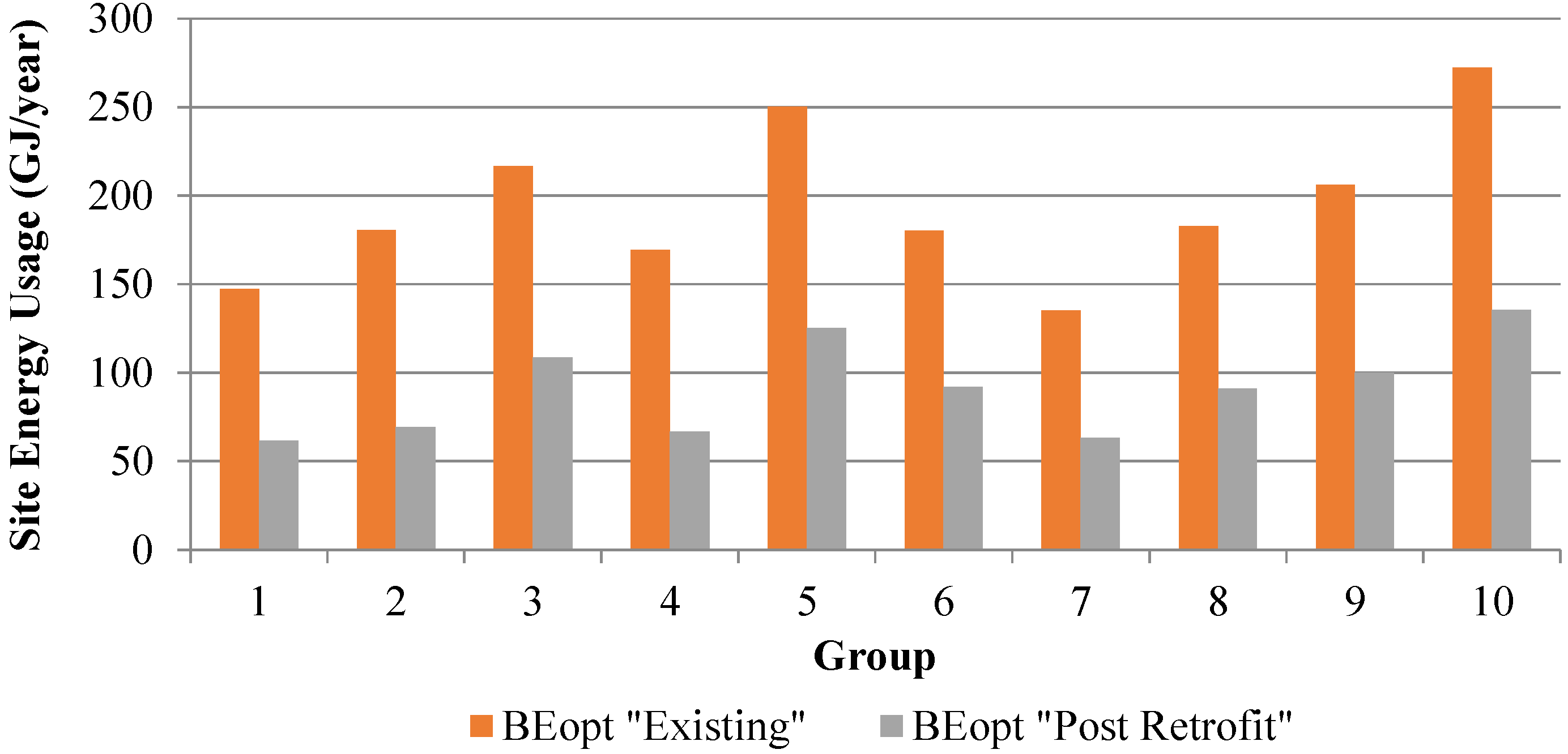
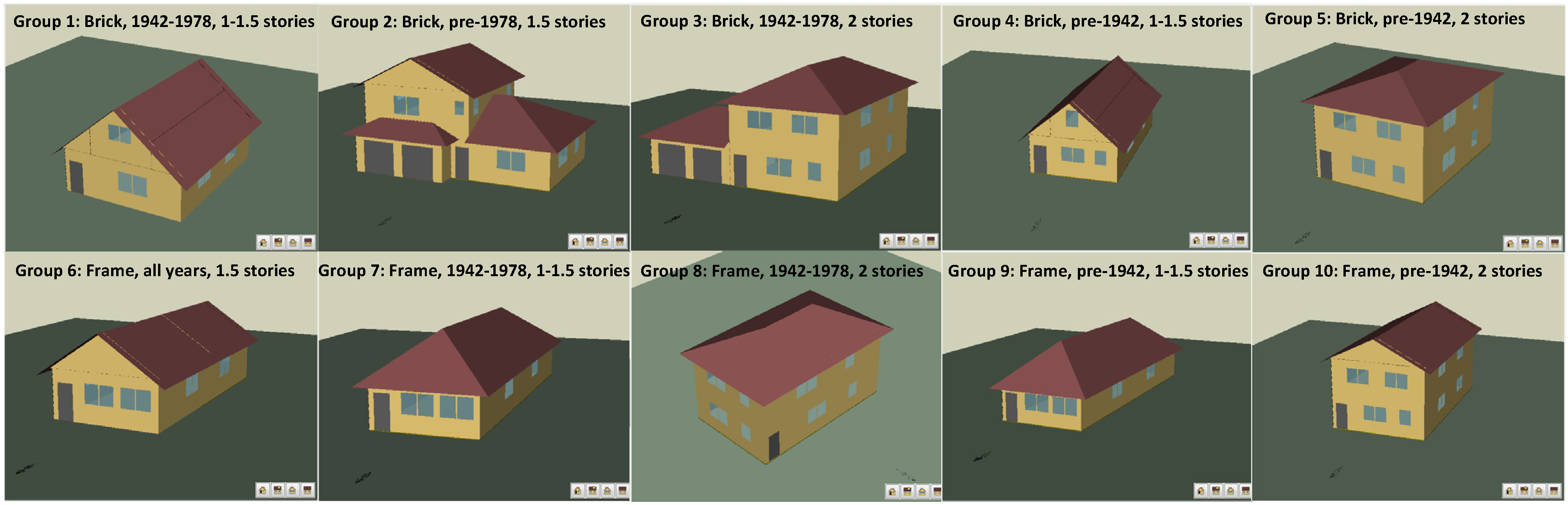
A recent study by the Partnership for Advanced Residential Retrofit (PARR) surveyed the Chicagoland residential housing stock and identified 15 common single-family housing typology groups that accurately represent the vast majority of single-family homes in the area [18]. The groups were characterized based on data collected from the Cook County assessors, utility billing history, and prior energy efficiency programs. One of the goals of the PARR report was to identify energy efficiency solutions to yield 30% annual energy savings using a simulation-based optimization approach that relied on just one generally representative home model for each of the 15 groups. Here we advance this previous work by considering the 10 least efficient typology groups of single-family homes out of the original group of 15 home types (all built prior to 1978) for finding cost-optimal deep energy retrofit packages that can achieve 50% annual site energy reductions. The 10 typology groups are represented by individual home models with the following characteristics, listed according to exterior wall structure, time period of construction, number of stories, and average floor area:

• Group 1: Brick, 1942–1978, 1–1.5 stories (no split level), 110 m² (1180 ft²)
• Group 2: Brick, Pre-1978, Split level (1.5 stories), 120 m² (1310 ft²)
• Group 3: Brick, 1942–1978, 2 stories, 190 m² (2060 ft²)
• Group 4: Brick, Pre-1942, 1–1.5 stories (no split level), 110 m² (1140 ft²)
• Group 5: Brick, Pre-1942, 2 stories, 170 m² (1870 ft²)
• Group 6: Frame, All years, Split level (1.5 stories), 120 m² (1340 ft²)
• Group 7: Frame, 1942–1978, 1–1.5 stories (no split level), 110 m² (1180 ft²)
• Group 8: Frame, 1942–1978, 2 stories, 150 m² (1580 ft²)
• Group 9: Frame, Pre-1942, 1–1.5 stories, 120 m² (1240 ft²)
• Group 10: Frame, Pre-1942, 2 stories, 190 m² (2060 ft²)

Full details of these home characteristics are described in the original PARR report [18], which also demonstrates how the individual home models accurately represent the average home in each group. A few adjustments were made to the base model inputs to yield reasonably accurate predictions of annual source and site energy use when compared to average utility bills from each home group reported in [18]. We targeted pre-retrofit simulation accuracy of within 20% of the average annual source energy use, electricity use, and natural gas consumption from each group simulated in the PARR report and we were successful in replicating pre-retrofit results for each home group within this defined range. The only deviations from [18] included modeling Group 1 homes with slab construction, Group 4 with a floored attic, and Group 9 with R-3 attic insulation. Otherwise, the same model inputs for 10 of the representative home types were used for energy simulation and optimization in the BEopt software package, as described in Section 2.2. Screenshots of each home model are shown in Figure 1.

Figure 1. Screen capture of representative homes from the 10 typology groups as modeled in BEopt.

Figure 1. Screen capture of representative homes from the 10 typology groups as modeled in BEopt.

2.2. Model Inputs for BEopt

2.2.1. General Assumptions

BEopt Version 2.2.0.2 was used with EnergyPlus 8.1.0 as the simulation engine to model each home type. The following general assumptions were applied to all home models, in direct alignment with the PARR report [18]:

• Lot size, distance to neighbors, and orientation were based on homeowner input from the PARR research team and information of a standard city and suburban lot with all homes facing north.
• The heating set point was set at 21.1 °C (70 °F) and the cooling set point was 22.2 °C (72 °F).
• All windows were modeled as double-clear (i.e., window glass plus storm window) in all cases. Note that there is not a “Double-Clear” window option in the BEopt version used for this work, but a custom option was created based on the same parameter from a previous version (BEopt version 1.0).
• Mechanical ventilation was modeled as “none” for pre-1942 homes and “spot ventilation” for the other vintages (i.e., spot exhaust fans in kitchen and bathrooms). This parameter option was also not included in the newest version of BEopt and was created based on BEopt version 1.0 parameter with the same name.
• All homes were modeled with the assumption that they were fitted with relatively modern appliances to reflect common energy upgrades typically made to houses over time (i.e., pre-1942 homes were not assumed to have appliances from 1942 but were assumed to have upgraded appliances more consistent with 10–20 year old vintages).
• Typical usage was assumed for miscellaneous electrical loads for all groups (i.e., “Other Electrical Loads” were set at “1.00”).

Next, assumptions for relevant characteristics of each home typology are described, including wall and roof construction type and insulation level, envelope airtightness, and HVAC system type and efficiency. They all assume the same “today” conditions from the PARR report [18] (i.e., very old homes were assumed to have undergone at least minor energy efficiency retrofits within the last 50 years to bring their performance closer in line with what is observed in Chicago area homes).

2.2.2. Detailed Assumptions: Pre-1942 Construction (Groups 4–6, 9, and 10)

Detailed assumptions for existing homes built prior to 1942 are as follows. Brick walls (Groups 4 and 5) were double brick construction with enclosure layers from outside to inside as: 10.2 cm (4 inch) brick, 2.5 cm (1 inch) airspace (the weep space, largely mortar and bricks connecting the inside and outside layer), an inside brick layer, wood lath with no insulation in the spaces, and 1.6 cm (5/8 inch) drywall simulating plaster. A structural brick wall was not a default option in BEopt, so a custom option was made based on concrete masonry unit (CMU) structured walls (15.2 cm (6 inch) hollow CMU) with the same physical specifications as brick. Costs associated with these options were carried over from the CMU base. Wood frame walls (Groups 6, 9, and 10) were modeled from the outside to inside as: siding, sheathing, 38 × 89 mm (2 × 4) uninsulated walls, and 1.6 cm (5/8 inch) drywall. Attic insulation was assumed to be a minimal RSI-1.2 (R-7). Bungalows were modeled with finished attic space in the upper half story. Inter-zonal knee-walls were modeled with no insulation and the roof above the living space was also modeled with no insulation. Basements were modeled as uninsulated as well. Enclosure airtightness assumptions were “very leaky” for 1-story and “leaky” for 2-story homes. Boilers with 80% efficiency were used for heating systems (representing common efficiencies from the 1980s) and window air-conditioning units with a coefficient of performance (COP) of 2.93 (energy efficiency ratio, or EER, of 10) were assumed for cooling systems. Gas water heaters were assumed with an energy factor of 0.48, and a gas dryer was also assumed.

2.2.3. Detailed Assumptions: 1942–1978 Construction (Groups 1–3, 7 and 8)

Detailed assumptions for existing homes built between 1942 and 1978 were as follows. For brick walls (Groups 1–3), 2.5 cm (1 inch) of RSI-0.5 (R-3) fiberglass was included between furring strips. For wood frame (Groups 7 and 8) and inter-zonal walls, an RSI-1.2 (R-7) fiberglass batt was modeled as the typical insulation level for that era. Attic insulation was assumed to be RSI-3.4 (R-19). Envelope airtightness was upgraded to “leaky” for 1-story homes and “typical” for 2-story homes. Gas furnaces with AFUE of 78% were assumed to have replaced boilers in the average house in this time frame. Central cooling systems were modeled with a COP of 2.6 (EER = 8.9). Gas water heaters were assumed with energy factors (EF) of 0.48. Additionally, a special case assumption was applied to improve the accuracy of the existing model for Group 1. The majority of houses in this group had slab floor construction (no basement), which best fit the measured annual energy use intensity [18]; therefore, slab construction was modeled in this case only.

2.3. Retrofit Optimizations Using BEopt and EnergyPlus

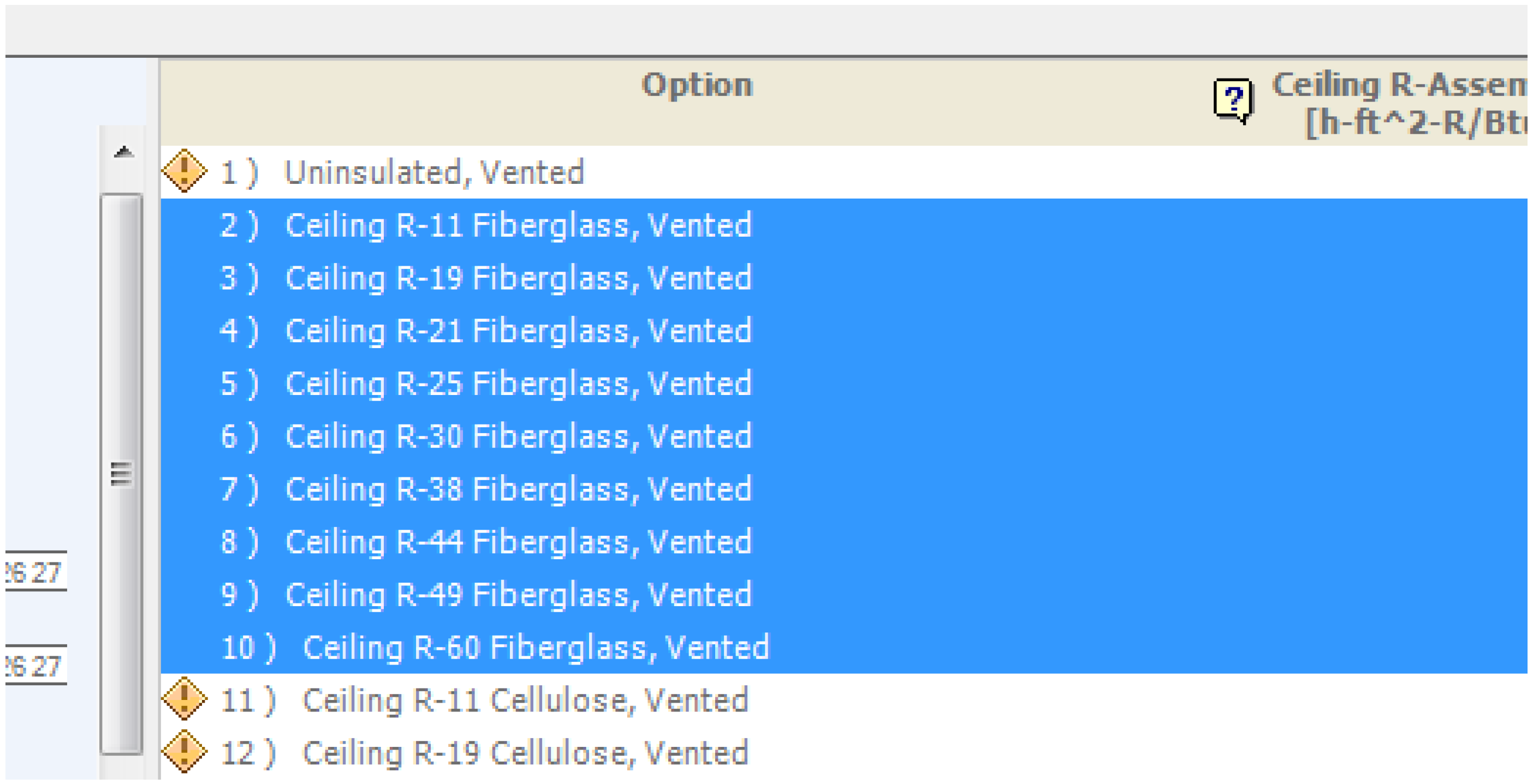
BEopt was used in “optimization mode”, which allows users to select pre-defined ranges of a number of model input parameters to consider for optimization (Figure 2 shows an example of ceiling assembly options from just one scenario). BEopt then performs energy simulations using a sequential search method to vary across all selected inputs and march towards a cost-optimal savings solution [20]. The sequential search method involves systematically applying permutations of all selected ranges of input parameters and searching for the most cost-effective option at each sequential point along the path towards zero net energy use. The method seeks the steepest downward slope along a least cost line to identify solutions that provide the most energy savings for the least amount of investment. Upfront material and construction costs for each retrofit measure were kept as default values in BEopt, which sources cost information from R.S. Means and other databases [20]. Based on the results, the most cost-effective option is selected as an optimal point on the path and included in an updated building configuration. The process is repeated until a specified desired outcome is reached (e.g., a user-defined source energy, site energy, or green house gas emissions reduction target). Each distinct simulation represents an “iteration point”, or a unique building configuration.

Figure 2. Screenshot of BEopt option list illustrating valid and invalid options for retrofit optimizations.

Figure 2. Screenshot of BEopt option list illustrating valid and invalid options for retrofit optimizations.

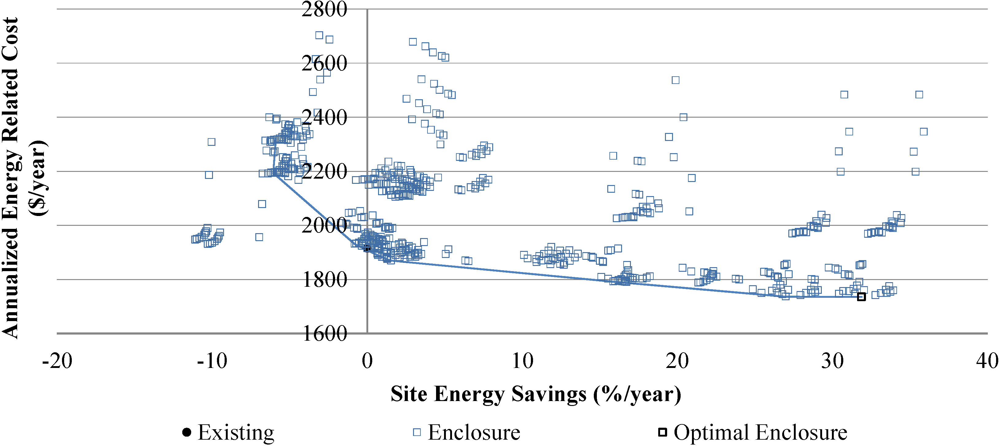
We began our optimizations for each typology group by selecting only building enclosure retrofit options in order to identify the least cost packages for reducing heating and cooling loads prior to seeking higher efficiency HVAC solutions. This is a common approach to identifying whole-house energy efficiency retrofit packages: reduce loads, and then improve equipment [21]. This approach also served to drastically reduce the computation time required to perform the simulations. Subsequently, optimizations based on the envelope-retrofitted models were then performed using a range of several HVAC system type and efficiency options. We then used the combined results to identify final cost-optimal packages for each home model representing its typology group as those that achieve at least 50% site energy savings while minimizing annualized energy related costs (AERC) and simple payback periods and providing the highest modified internal rate of return (MIRR). In each case, parameter options that BEopt deemed inappropriate or ineligible, including those for which costs could not be calculated, were denoted by an exclamation mark next to the option on the options selection screen (e.g., options 1, 11, and 12 in Figure 2). These options were not selected for use in the optimizations.

Possible building enclosure optimization options for each group included the following:

• Exterior Wood Stud Walls (Groups 6–10): For homes with frame exterior wall constructions, all higher thermal resistance options for exterior walls that were deemed valid/eligible by BEopt were chosen for optimization. These included most default 38 × 89-mm (2 × 4), 40.6 cm (16 inches) on center (o.c.) framing options insulated with fiberglass batt, blown-in cellulose, blown-in fiberglass, or spray foam insulation. Possible insulation levels ranged from RSI-1.2 m²·K/W (R-7 h∙ft²∙°F/Btu) (fiberglass batts) to RSI-4.1 (R-23) (spray foam).
• Exterior Brick Walls (Groups 1–5): For homes with brick exterior wall constructions, new CMU options for the weep space plus 10.2-cm (4-inch) interior brick were created based off existing 15.2-cm (6-inch) hollow CMU options (BEopt does not have built-in double brick wall options). All specifications for the masonry (i.e., block thickness, material conductivity, and density) were modified to reflect the specifications of brick, but all labor and material costs associated with the original default options were kept as defaults for the new brick options. These options include the double brick wall insulated with either of the following insulation types/levels within the interior side furring cavity: RSI-0.53 (R-3) fiberglass batt (5.1-cm or 2-inch furring cavity), RSI-1.76 (R-10) XPS (5.1-cm or 2-inch furring cavity), RSI-2.3 (R-13) closed cell spray foam (5.1-cm or 2-inch furring cavity), RSI-2.1 (R-12) polyiso (5.1-cm or 2-inch furring cavity), or RSI-3.3 (R-19) fiberglass batt within a 38 × 140 mm (2 × 6), 60.9 cm (24 inches) o.c. furring cavity.
• Wall Sheathing (Groups 6–10): For homes with frame exterior wall constructions, the following insulation options were chosen for optimization as being installed between the exterior finish and the frame wall: RSI-0.9 (R-5) XPS, RSI-1.8 (R-10) XPS, RSI-2.6 (R-15) XPS, RSI-1.1 (R-6) polyiso, and RSI-2.1 (R-12) polyiso.
• Exterior Finish: All colors for the appropriate finish were chosen (i.e., light or medium/dark brick for brick constructed homes, and light or medium/dark wood siding for frame constructed homes).
• Interzonal Walls: In groups where interzonal walls are present, all eligible options for 38 × 89 mm (2 × 4) 40.6 cm (16 inches) o.c. interzonal walls were chosen. This included walls insulated with either fiberglass batt, blown-in cellulose, blown-in fiberglass, or spray foam insulation, with insulation levels ranging from RSI-1.2 (R-7) (fiberglass batts) to RSI-4.1 (R-23) (spray foam).
• Unfinished Attic: In groups where unfinished attic space was present, all eligible BEopt options were chosen for optimization. Specific options varied by group and were dependent mainly on vintage and existing insulation. Options were considered appropriate if they represented an improvement in thermal resistance. Selected options included but were not limited to options with insulation installed in either the attic floor space (ceiling of the finished space), within the cavity space between 38 × 140 mm (2 × 6) rafters (roof), or both ceiling and roof (in a few cases). Insulation in the form of vented, blown-in fiberglass; vented, blown-in cellulose; fiberglass batt; or closed cell spray foam in the ceiling space, and/or closed cell spray foam in the roof were chosen with R-values ranging from RSI-1.9 (R-11) to RSI 10.6 (R-60) for both types of insulation.
• Finished Roof: In groups where finished attic space was present, all eligible options with an R-value greater than or equal to the existing levels were considered, including the existing insulation, RSI 3.3 (R-19) blown-in fiberglass within 38 × 140 mm (2 × 6) rafters, both alone and in combination with XPS having thermal resistance of RSI-2.6, 3.5, or 4.4 (R-value of 15, 20, or 25).
• Roof Material: For all groups, the options chosen for roof material included “Asphalt shingles” in all default colors: dark, medium, light, or white or cool colors.
• Radiant Barrier: For all groups, both the available options for this parameter were chosen; “none” (the existing condition), or “double-sided, foil”.
• Unfinished Basement: All default options for insulating and finishing of the basement interior perimeters were chosen for all groups.
• Interzonal Floor: Interzonal floors separate conditioned from unconditioned space (e.g., the floor separating the unfinished attic from the conditioned space below, or the ceiling area/floor area between the unconditioned garage and conditioned living space above). In models of groups for which interzonal floors were present, all default options were selected for optimization with this parameter.
• Window Type: For all groups, all eligible window options were chosen for optimization. This includes all double or triple pane; low, medium, or high gain low-e coated; insulated or non-metal frame; and air or argon filled configurations. An option for backside windows (i.e., south facing) to have a high solar heat gain coefficient (SHGC) was also included among the options chosen for optimization.
• Air Leakage: Options selected for the air leakage parameter was dependent on group vintage and number of stories. Only the existing condition and the option that represented a single step up were chosen for each group (e.g., “very leaky” to “leaky”, “leaky” to “typical”, or “typical” to “tight”), as two-step upgrades were not assumed to be realistic for the pre-1978 vintage [18].
• Mechanical Ventilation: The selection of options for mechanical ventilation parameters was dependent on group vintage. For pre-1942 groups, all default options were selected, but for 1942–1978, all eligible options were selected for optimization. “Supply” and “supply, 50% of ASHRAE 62.2” options were not deemed eligible for simulation for the latter vintages.

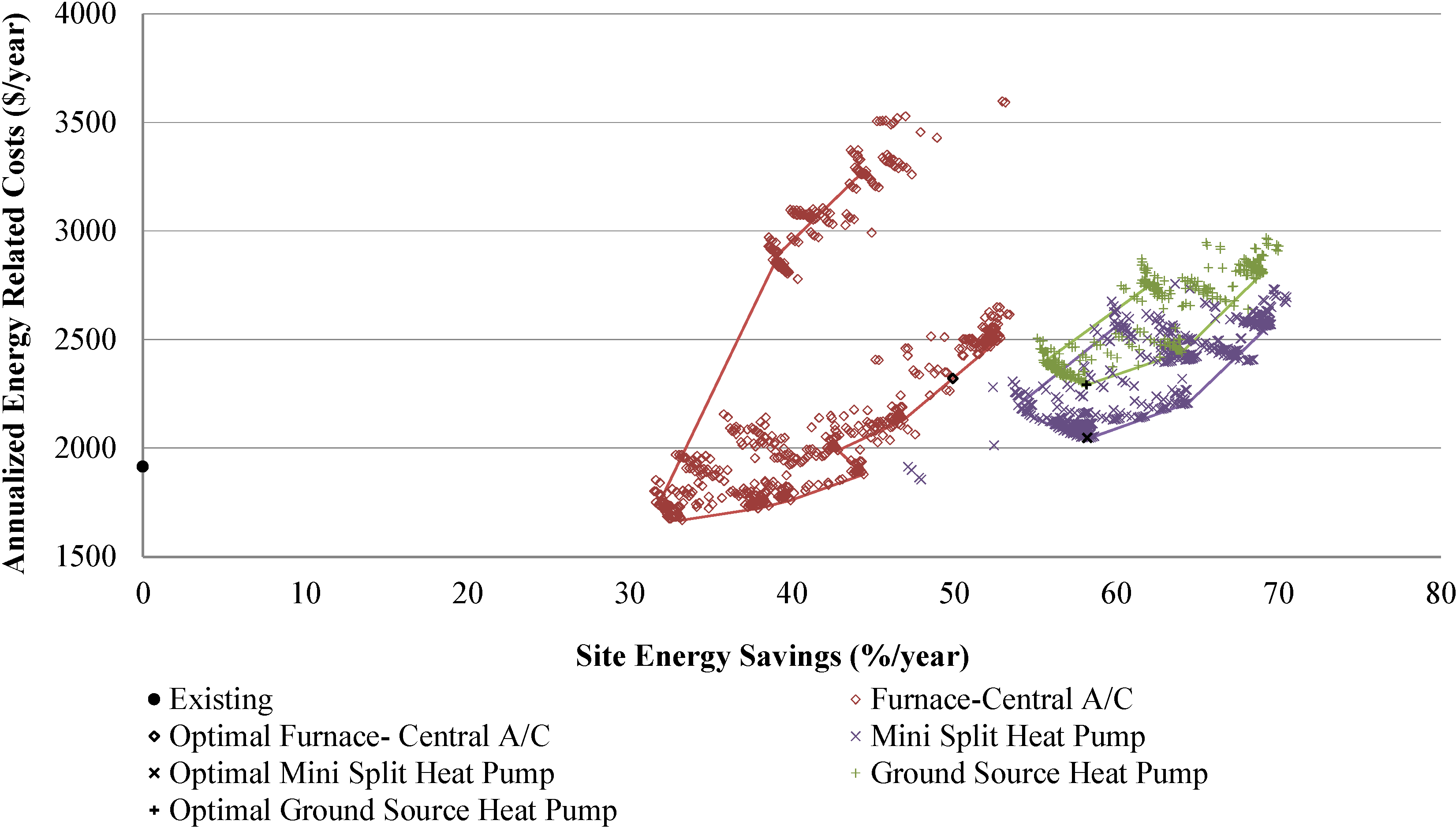
Once optimal cost-effective enclosure retrofits were identified, another set of simulations was conducted using the following options as possible HVAC system types and characteristics:

• Central A/C: Options that represented improvements to the existing central air-conditioning (A/C) system efficiency were deemed eligible by BEopt. All default options with a COP equal to or higher than 2.6 (EER equal to or higher than 8.9) were chosen for optimizing central A/C systems.
• Room A/C: All BEopt default options for room A/C parameters were deemed eligible and were only utilized for pre-1942 groups with existing boiler and room A/C combinations (Groups 4–6, 9, and 10).
• Furnace: Only options that represented improvements to the existing furnace efficiency were deemed eligible and selected for optimization. Options include gas furnaces with AFUE ratings of 78% and above (up to 98%) and an electric furnace with an AFUE of 100%.
• Boiler: Similar to the A/C and furnace parameters, the options chosen for optimization with boilers included only those that represent an improvement to the existing boiler efficiency. This includes both condensing and non-condensing gas boilers with an AFUE of 80% and higher (up to 98%). Boiler parameters were only utilized for pre-1942 groups with existing boiler and room A/C combinations (Groups 4–6, 9, and 10).
• Mini-Split Heat Pumps (MSHP): All default options were selected for optimizing mini-split heat pump systems for all groups.
• Electric Baseboards: BEopt requires for electric baseboard heaters to be selected when simulating MSHP system options; thus, the default option of 100% efficiency was chosen for electric baseboard heater optimizations.
• Ground-Source Heat Pumps (GSHP): Chicago’s close proximity to Lake Michigan has a large influence on the thermal conductivity of the area’s soil and thus the potential to incorporate geothermal heating in the form of ground-source heat pumps (GSHPs) into homes. The soil of the entire Chicago area can be classified as illitic or silty/clayish [22]. The thermal conductivity of saturated silt/clay soil has a thermal conductivity within the range of 1–1.8 W/mK for saturated unfrozen soil and 2–2.5 W/mK for saturated frozen soil [23]. From this information, an average soil thermal conductivity of 1.8 W/mK was used, which corresponds to high conductivity soil in BEopt.
• Ducts: The options deemed eligible for optimization by BEopt depended on vintage and the presence of pre-existing ductwork. For groups without pre-existing ductwork (pre-1942 homes including Groups 4–6, 9, and 10), all default options were selected. For all remaining groups (all 1942–1978 groups), only options that represented an increase in thermal resistance or a decrease in duct leakage from the existing conditions were selected, including both insulated and uninsulated ducts with leakage fractions of 15% or less, as well as an option to relocate ducts to finished space. These parameters were only applied to ducted HVAC systems (e.g., furnace-central A/C combinations and GSHP scenarios).

An air-source heat pump (ASHP) case was also initially included among the HVAC systems simulated for optimization. However, conventional ASHPs have been recommended for use mostly in more moderate climates because the effectiveness of ASHPs begins to degrade substantially as outdoor temperatures fall below −8 °C (~17.6 °F) [24]. Moreover, it has been reported that most ASHP systems shut off when ambient temperatures reach freezing and switch to backup heating [25]. Since the average mean seasonal temperature for the Chicago area winters in the past decade is 26.1 °F (−3.2 °C) [26], it was determined that the implementation of ASHP systems would indeed necessitate a backup heating system. However, supplemental heat could not be accurately modeled in BEopt simultaneously with ASHPs, as the methods of heating are considered to be mutually exclusive, unfortunately. While advancements have been made to increase feasibility of their implementation in cold climates [27], the developers of BEopt have yet to make cold climate ASHP options available/appropriate for simulation [28]. Therefore, the results of the simulations involving this particular system were ultimately considered invalid and not used herein.

Finally, the following non-HVAC and non-enclosure options were selected for all cases in all groups:

Ceiling Fan: All default options for ceiling fans were deemed eligible by BEopt; however, the options selected for optimization were limited to “none”, “benchmark”, “standard efficiency”, “high efficiency”, and “premium efficiency” ceiling fans.

d.

Water Heater: Options that represented an improvement in efficiency from the existing conditions were deemed eligible. Only those water heaters that operate using gas, electric, or heat pump water heater (HPWH) options were selected.

d.

Solar Water Heating (SWH), SWH Azimuth, and SWH Tilt: All default options for these parameters were considered appropriate and selected for optimization.

d.

Lighting: Lighting options were deemed eligible by BEopt if they consumed less electricity than the existing case and were thus selected for optimization. Included are options for 40% to 100% hardwired lighting to be converted to fluorescent lighting, 40%–100% hardwired and plug-in lighting to be converted to fluorescent lighting, conversion of 50% hardwired and plug-in lighting to fluorescent and 10% to Light-Emitting Diode (LED), and fixed annual lighting electricity consumption allowance of 1300 kWh/year (achieved by any combination of lighting technologies).

The simulations did not include analysis of any building user preference or behavior parameters such as natural ventilation, shading, or large appliances other than water heaters and HVAC equipment (e.g., refrigerators, washers, dryers, etc.). The simulations also did not include analysis of any building characteristics that are not practical to change, such as building orientation and distance from neighbors. The options for these parameters were selected based either on PARR assumptions, options that best fit measured or reported annual energy use in the PARR report (e.g., less efficient appliances were chosen to accurately reflect measured energy usage as needed), or BEopt defaults, and left unchanged throughout the simulation processes. For all simulations, the EnergyPlus weather location was set as “USA_IL_Chicago-OHare.Intl.AP.725300_TMY3.epw”. Moreover, as the scope of this work includes the entire Chicagoland area, which includes several near suburbs, therefore, the terrain was set to “Suburban” for all simulations.

The most recent release of BEopt (version 2.2) was equipped with capabilities for user-specified utility rates. For the modeling purposes of this work, a Real-Time-Pricing (RTP) electricity cost profile was created based on actual RTP costs from the local electric utility, ComEd, for the year of 2012 [29]. RTP was used instead of average block pricing because utilities are changing to this method (albeit more slowly in some locations compared to others). For natural gas pricing, an average of the monthly residential cost of gas found on the website of the local natural gas utility (Nicor Gas) was used [30]. All other values for economic assumptions (e.g., inflation rate, discount rate, etc.) and payment assumptions (e.g., loan interest rate, loan period, marginal income tax rate, etc.) were left as the BEopt default values.

The goal of this work was to identify packages that achieve a 50% site energy savings (i.e., only the energy used on-site without accounting for primary energy conversion efficiencies). However, the final BEopt optimization simulations were actually set to terminate when a 50% source energy savings was achieved, or otherwise continue the simulations until all possible input parameter combinations were exhausted. This was done primarily because a source energy reduction of 50% would ensure that at least a 50% site energy reduction was achieved, given that the source/site conversion ratios were kept at the BEopt default values of 3.15 for electricity and 1.09 for natural gas. This allowed for identifying packages with even higher site energy savings than 50% that were still cost-effective options. Ultimately none of the simulations achieved 50% source energy savings, so each optimization case actually provided an exhaustive search over all selected input parameters.

Initial BEopt simulations were performed in a Virtual workstation running Windows 7 Professional on a MacBook Air equipped with a 1.8 GHz Intel Core i7 processor and 4 GB 1333 MHZ DDR3. The first simulation was allowed to run for about 15 h, during which only eight “iterations”, or 1249 unique simulations (or “iteration points”), were completed before the test was manually terminated. Given this duration, we then decided to outsource simulations to a remote server on the Amazon Elastic Compute Cloud (EC2). For all subsequent simulations, a “C3 High-CPU Eight Extra Large” (c3.8xlarge) instance with 108 compute units, 32 cores, and 60 GB of memory was used to allow for more rapid remote simulations. The chosen instance was setup to use the latest Microsoft Windows Server operating system and BEopt was installed just as it would be on a typical PC computer. Simulations were managed though the Microsoft Remote Desktop application installed on the previously mentioned MacBook. The simulation run time was reduced down to about 1.5 h per optimization simulation case using Amazon EC2 (a case being defined as a set of simulations performed to optimize a particular home type and enclosure or type of HVAC retrofit combination). Ultimately, each group model involved the optimization of a minimum of four cases (e.g., one enclosure optimization case and at least three different HVAC system optimization cases), with each case having a minimum of nine iterations with any individual iteration points. Some cases required the simulation of upwards to 25 iterations with a mean number of about 15 iterations per case. Using the mean 15 iterations per case, it was calculated that it would have required a minimum of about 1125 h to complete simulations on the aforementioned MacBook personal computer. Using Amazon EC2, the required minimum run time was reduced to about 80 h, yielding a ~93% reduction in run time to complete simulations. Similar cloud computing approaches have been used in other recent studies as well [31,32].

3. Results and Discussion

Examples of typical inputs and outputs from the simulations are shown for just one home typology in Section 3.1 (Group 1). This serves to demonstrate the nature of the inputs required for this process and the resulting outputs for each group. Results from all home types are then explored and summarized in Section 3.2, Section 3.3 and Section 3.4.

3.1. Demonstration of Results from Group 1 (Brick, 1942–1978, 1–1.5 Stories, No Split Level)

Figure 3 shows full BEopt geometry inputs for the Group 1 representative home. After the base model and existing conditions were modeled for each home type and compared to results from those in the PARR report [18], building enclosure optimization simulations were then performed for each home. The simulations were set to terminate when the least cost package of all possible combinations of the selected parameter options was found. Figure 4 illustrates the results of the enclosure optimization simulation for the Group 1 home type based on annualized energy related costs (AERC) compared to site energy savings, along with the least cost fit line generated by the sequential search optimization method in BEopt. AERC combines the upfront costs of retrofits with the predicted resulting annual energy savings accumulated over the project analysis period (assumed to be the BEopt default of 30 years) and calculates an annualized cost metric for comparing scenarios. Each square symbol in Figure 4 represents a single combination of enclosure parameters or iteration point and the AERC for the existing home as-is (i.e., savings = 0%) is shown with a black circle. Ideally, the most desirable packages would be present in the lower right portion of the graph, with large energy savings and low annualized costs.

In this case, the least cost option that was identified as cost-optimal represents an estimated site energy savings of about 32% with an AERC of about $1740 per year (compared to an AERC in the existing home of about $1915 per year). These results demonstrate that considerable energy savings may be achieved in this home type simply by upgrading the enclosure and keeping the existing HVAC systems (the selected enclosure retrofit details are described in full in Section 3.2). It can also be seen that the least cost option has an AERC that is almost $200 per year less than the existing case for this group. In short, it pays in the long run to install the optimal enclosure retrofits.

Figure 3. BEopt model for Group 1: Foundation, first, and second (attic) floor layouts and 3D view.

Figure 3. BEopt model for Group 1: Foundation, first, and second (attic) floor layouts and 3D view.

Figure 4. Building enclosure optimization results for Group 1 homes.

Figure 4. Building enclosure optimization results for Group 1 homes.

After the optimal enclosure retrofits were implemented, the model was then optimized for various HVAC systems in order to advance beyond 32% site energy savings. For Group 1 homes, this included the existing HVAC systems (combination of a furnace and central A/C), mini split heat pump (MSHP), and ground source heat pump (GSHP). Figure 5 shows the results for the HVAC optimization simulations for this group alongside the corresponding least cost fit line generated by the sequential search optimization method in BEopt. Similar to the enclosure results, optimal packages are those that maximize energy savings while minimizing AERC. For each HVAC case, the lowest cost iteration point along the least cost fit line that achieved an annual energy use reduction greater than 50% was chosen as the cost-optimal deep energy retrofit solution (i.e., the MSHP case in Figure 5). This ensured that the package with the combined lowest AERC, highest energy savings, shortest payback period, and highest modified internal rate of return was chosen.

Note that in this example, the optimal package occurs at about 58% site energy savings for both the MSHP and the GSHP systems. Also note that in this example, there are several iteration points that represent options that have a lower AERC than the option chosen to be the optimal MSHP package but are not considered to be part of the least cost fit line. Further inspection revealed that BEopt does not consider these options to be least cost options because they were estimated to have higher payback periods than the cost-optimal package shown in Figure 5, despite the lower AERC. Moreover, the optimal package for the furnace-central A/C combination that represents the least cost at 50% savings occurs at an AERC that is higher than the absolute minimum of the least cost line for this HVAC system. Thus, Figure 5 demonstrates that the optimal retrofit package involves application of the enclosure retrofits from Figure 4 combined with conversion to a MSHP, which is predicted to yield an increase in AERC of only about $135 per year ($2050 per year compared to the original $1915 per year). In this particular home, enclosure retrofits are predicted to have net economic benefits (lower AERC than existing) but cannot achieve 50% energy savings, while additional upgrades to the HVAC system would yield greater than 50% energy savings albeit at a small additional annual cost (higher AERC).

Figure 5. HVAC optimization results for Group 1 homes.

Figure 5. HVAC optimization results for Group 1 homes.

Next, Figure 6 illustrates the breakdown of estimated energy consumption by end use for the Group 1 model, including the predicted energy use at the existing/current condition, after the implementation of optimal enclosure, and for each of the optimal HVAC packages in combination with the optimal enclosure package. Again, it is clear that the conversion to a MSHP is estimated to result in the greatest energy savings out of all simulated options for this particular group. The majority of savings stem from a reduction in heating energy consumption.

Figure 6. Site energy use of critical optimal iteration points for Group 1 homes.

Figure 6. Site energy use of critical optimal iteration points for Group 1 homes.

Finally, there are two additional metrics to compare the overall costs and benefits of optimal retrofit packages for each home type. First, the “simple payback period” of a project represents the time required for a repayment of the original investment, but does not incorporate future costs (e.g., replacement costs or technology upgrades), future changes to cost savings (e.g., utility cost changes due to fuel price escalation), or the time value of money or loan financing. Figure 7 illustrates the simple payback periods for each of the optimal HVAC packages (combined with the optimal enclosure) for Group 1 homes. When combined with the optimal enclosure retrofit, a conversion to MSHP in this home is predicted to yield annual site energy savings of 58.2% (the same values shown in Figure 5 and Figure 6) with a simple payback period of about 24 years. Further, this represents a modified internal rate of return (MIRR) of about 3.8%. These two metrics can help homeowners and decision makers better understand the costs and benefits of their investments. While a 24-year simple payback period seems like a long period of time, an MIRR of 3.8% is actually much higher than the current rate of return on, for example, U.S. savings bonds.

Figure 7. Simple payback period of critical optimal iteration points for Group 1 homes.

Figure 7. Simple payback period of critical optimal iteration points for Group 1 homes.

3.2. Optimal Cost-Effective Prescriptive Retrofit Packages for Each Pre-1978 Home Typology Group

A summary of the cost-optimal prescriptive deep energy retrofit packages resulting from the two-step optimization process applied to all 10 typology groups is shown in the following tables (Table 1, Table 2, Table 3, Table 4, Table 5, Table 6, Table 7, Table 8, Table 9 and Table 10). Metrics for evaluating and comparing each retrofit package include: initial costs, annualized energy related costs (AERC), predicted site and source energy savings, simple payback periods, and the modified internal rate of return (MIRR).

Group 1: The cost-optimal retrofit package for Group 1 homes calls for an increase in exterior wall insulation (from RSI-0.53 to RSI-3.3 using fiberglass batts within a thicker wall construction) and unfinished attic insulation (improved to blown-in closed cell spray foam insulation), an increase in air tightness of the enclosure (from “leaky” to “typical”), and a conversion from the existing furnace and central A/C system to a high-efficiency MSHP system with electric baseboard heating (Table 1). It was also recommended that 100% of the lighting be converted to fluorescent bulbs for both hardwired and plug-in fixtures. A more energy efficient water heater was not found to be a cost-effective upgrade for this particular group. The total upfront costs of this optimal retrofit package is predicted to be about $11,200, providing ~58% site energy savings with a simple payback period of 24 years and a MIRR of 3.8%. Ultimately, greater than 50% energy savings can likely be achieved in this home with additional annualized energy-related costs of only about $132 per year.

Table 1. Group 1: Brick, 1942–1978, 1–1.5 stories (no split level) Summary of retrofit package and cost and energy conservation implications.

Parameter name	Existing characteristics	Optimal enclosure + HVAC retrofit package
Exterior Wall (Masonry)	10.2-cm Hollow Brick, RSI-0.53 Fiberglass Batt, 2.5-cm furring, 61 cm o.c.	10.2-cm Hollow Brick, RSI-3.3 Fiberglass Batt, 38 × 140 mm, 61 cm o.c.
Unfinished Attic	Ceiling RSI-3.3 Fiberglass (Blown-in), Vented	Roof RSI-3.3 Closed Cell Spray Foam
Air Leakage	Leaky	Typical
Central A/C	COP 2.6	None
Furnace	Gas, 78% AFUE	None
Electric Baseboard	None	100% Efficiency
Mini Split Heat Pump	None	COP 6.1, Avg Seasonal COP 3.2
Ducts	Typical, Uninsulated (Unfinished Attic)	None
Water Heater	Gas 54% EF	No Change
Lighting	Benchmark	100% Fluorescent, Hardwired & Plug-in
Initial Cost ($)	$0	$11,242
AERC ($/year)	$1915	$2047
% Site (Source) Energy Savings	0	58.2% (39.9%)
Simple payback period (years)	N/A	24 years
Modified internal rate of return (MIRR, %)	N/A	3.8%

Table 1. Group 1: Brick, 1942–1978, 1–1.5 stories (no split level) Summary of retrofit package and cost and energy conservation implications.

Parameter name	Existing characteristics	Optimal enclosure + HVAC retrofit package
Exterior Wall (Masonry)	10.2-cm Hollow Brick, RSI-0.53 Fiberglass Batt, 2.5-cm furring, 61 cm o.c.	10.2-cm Hollow Brick, RSI-3.3 Fiberglass Batt, 38 × 140 mm, 61 cm o.c.
Unfinished Attic	Ceiling RSI-3.3 Fiberglass (Blown-in), Vented	Roof RSI-3.3 Closed Cell Spray Foam
Air Leakage	Leaky	Typical
Central A/C	COP 2.6	None
Furnace	Gas, 78% AFUE	None
Electric Baseboard	None	100% Efficiency
Mini Split Heat Pump	None	COP 6.1, Avg Seasonal COP 3.2
Ducts	Typical, Uninsulated (Unfinished Attic)	None
Water Heater	Gas 54% EF	No Change
Lighting	Benchmark	100% Fluorescent, Hardwired & Plug-in
Initial Cost ($)	$0	$11,242
AERC ($/year)	$1915	$2047
% Site (Source) Energy Savings	0	58.2% (39.9%)
Simple payback period (years)	N/A	24 years
Modified internal rate of return (MIRR, %)	N/A	3.8%

Group 2: Similar upgrades were recommended for the Group 2 home (see Table 2), including increasing thermal resistance in the exterior walls (to RSI-3.3 fiberglass batts in thicker wall), interzonal walls (to RSI-2.3 blown-in fiberglass), and the unfinished attic (to RSI-4.4 blown-in fiberglass), improving the air tightness of the enclosure (from “leaky” to “typical”), and converting to 100% fluorescent lighting. A conversion to a MSHP and electric baseboard heating was also recommended for Group 2. The total upfront costs of this retrofit package is predicted to be about $11,200, providing ~61% site energy savings with a simple payback period of 23 years and a MIRR of 3.9%. Thus, greater than 50% energy savings can likely be achieved in this home with additional annualized energy-related costs of only about $144 per year.

Group 3: For Group 3 homes, similar upgrades to the enclosure insulation and airtightness were suggested (RSI-3.3 and RSI-4.4 wall and attic insulation, respectively, and increasing airtightness from “typical” to “tight”), as well as a conversion to 100% fluorescent lighting (see Table 3). However, unlike the previous two groups, an update to the existing furnace-central A/C system (from a COP of 2.6 to 6.5 and from 78% AFUE to 98%) was found to be cost-optimal. It was also recommended that the existing ductwork be moved from the typical location in the unfinished basement to finished space. Additionally, an update from the existing water heater to a tankless water heater was found to be a cost effective upgrade. The total upfront costs of this retrofit package is predicted to be about $17,500, providing ~50% site energy savings with a simple payback period of 15 years and a MIRR of 5.9%. In this home type, we predict that these energy savings goals can be met at an annualized energy-related cost that is actually about $84 per year lower than the existing home.

Table 2. Group 2: Brick, Pre-1978, Split level (1.5 stories) Summary of retrofit package and cost and energy conservation implications.

Parameter name	Existing characteristics	Optimal enclosure + HVAC retrofit package
Exterior Wall (Masonry)	10.2-cm Hollow Brick, RSI-0.53 Fiberglass Batt, 2.5-cm furring, 60.9 cm o.c.	10.2-cm Hollow Brick, RSI-3.3 Fiberglass Batt, 38 × 140 mm, 60.9 cm o.c.
Interzonal Walls	RSI-1.2 Fiberglass Batt, GR-3, 39 × 89 mm, 40.6 cm o.c.	RSI-2.3 Fiberglass (Blown-in), Gr-1, 39 × 89 mm, 40.6 cm o.c.
Unfinished Attic	Ceiling RSI-1.9 Fiberglass (Blown-in), Vented	Ceiling RSI-4.4 Fiberglass (Blown-in), Vented
Air Leakage	Leaky	Typical
Central A/C	COP 2.6	None
Furnace	Gas 78% AFUE	None
Electric Baseboard	None	100% Efficiency
Mini Split Heat Pump	None	COP 6.6, Avg Seasonal COP 3.3
Ducts	Typical, Uninsulated (Unfinished Basement)	None
Water Heater	Gas, 54% EF	No Change
Lighting	Benchmark	100% Fluorescent, Hardwired & Plug-in
Initial Cost ($)	$0	$11,190
AERC ($/year)	$2081	$2225
% Site (Source) Energy Savings	0	61.6% (40.8%)
Simple payback period (years)	N/A	23 years
Modified internal rate of return (MIRR, %)	N/A	3.9%

Table 2. Group 2: Brick, Pre-1978, Split level (1.5 stories) Summary of retrofit package and cost and energy conservation implications.

Parameter name	Existing characteristics	Optimal enclosure + HVAC retrofit package
Exterior Wall (Masonry)	10.2-cm Hollow Brick, RSI-0.53 Fiberglass Batt, 2.5-cm furring, 60.9 cm o.c.	10.2-cm Hollow Brick, RSI-3.3 Fiberglass Batt, 38 × 140 mm, 60.9 cm o.c.
Interzonal Walls	RSI-1.2 Fiberglass Batt, GR-3, 39 × 89 mm, 40.6 cm o.c.	RSI-2.3 Fiberglass (Blown-in), Gr-1, 39 × 89 mm, 40.6 cm o.c.
Unfinished Attic	Ceiling RSI-1.9 Fiberglass (Blown-in), Vented	Ceiling RSI-4.4 Fiberglass (Blown-in), Vented
Air Leakage	Leaky	Typical
Central A/C	COP 2.6	None
Furnace	Gas 78% AFUE	None
Electric Baseboard	None	100% Efficiency
Mini Split Heat Pump	None	COP 6.6, Avg Seasonal COP 3.3
Ducts	Typical, Uninsulated (Unfinished Basement)	None
Water Heater	Gas, 54% EF	No Change
Lighting	Benchmark	100% Fluorescent, Hardwired & Plug-in
Initial Cost ($)	$0	$11,190
AERC ($/year)	$2081	$2225
% Site (Source) Energy Savings	0	61.6% (40.8%)
Simple payback period (years)	N/A	23 years
Modified internal rate of return (MIRR, %)	N/A	3.9%

Group 4: The optimal retrofit package for Group 4 again includes upgrades to the enclosure insulation and air tightness, a conversion to 100% fluorescent lighting, and conversion to a MSHP (see Table 4). Exterior wall, interzonal wall, and ceiling insulation should be increased to RSI-3.3, RSI-2.3, and RSI-3.3, respectively, using fiberglass batts or blown-in fiberglass. Airtightness should be increased from “very leaky” to “leaky”, or higher. A water heater upgrade was not suggested for this group. The total upfront costs of this retrofit package is predicted to be about $10,500, providing ~61% site energy savings with a simple payback period of 31 years and a MIRR of 4.5%. For approximately $250 more in AERC, this home type is predicted to achieve energy savings beyond the original 50% target.

Table 3. Group 3: Brick, 1942–1978, two stories Summary of retrofit package and cost and energy conservation implications.

Parameter name	Existing characteristics	Optimal enclosure + HVAC retrofit package
Exterior Wall (Masonry)	10.2-cm Hollow Brick, RSI-0.53 Fiberglass Batt, 2.5-cm furring, 60.9 cm o.c.	10.2-cm Hollow Brick, RSI-3.3 Fiberglass Batt, 38 × 140 mm, 60.9 cm o.c.
Unfinished Attic	Ceiling RSI-1.9 Fiberglass (Blown-in), Vented	Ceiling RSI-4.4 Fiberglass (Blown-in), Vented
Air Leakage	Typical	Tight
Central A/C	COP 2.6	COP 6.5
Furnace	Gas, 78% AFUE	Gas, 98% AFUE
Ducts	Typical, Uninsulated (Unfinished Basement)	In Finished Space
Water Heater	Gas, 54% EF	Gas Tankless
Lighting	Benchmark	100% Fluorescent Hardwired & Plug-in
Initial Cost ($)	$0	$17,506
AERC ($/year)	$2430	$2346
% Site (Source) Energy Savings	0	49.9% (45.5%)
Simple payback period (years)	N/A	15 years
Modified internal rate of return (MIRR, %)	N/A	5.9%

Table 3. Group 3: Brick, 1942–1978, two stories Summary of retrofit package and cost and energy conservation implications.

Parameter name	Existing characteristics	Optimal enclosure + HVAC retrofit package
Exterior Wall (Masonry)	10.2-cm Hollow Brick, RSI-0.53 Fiberglass Batt, 2.5-cm furring, 60.9 cm o.c.	10.2-cm Hollow Brick, RSI-3.3 Fiberglass Batt, 38 × 140 mm, 60.9 cm o.c.
Unfinished Attic	Ceiling RSI-1.9 Fiberglass (Blown-in), Vented	Ceiling RSI-4.4 Fiberglass (Blown-in), Vented
Air Leakage	Typical	Tight
Central A/C	COP 2.6	COP 6.5
Furnace	Gas, 78% AFUE	Gas, 98% AFUE
Ducts	Typical, Uninsulated (Unfinished Basement)	In Finished Space
Water Heater	Gas, 54% EF	Gas Tankless
Lighting	Benchmark	100% Fluorescent Hardwired & Plug-in
Initial Cost ($)	$0	$17,506
AERC ($/year)	$2430	$2346
% Site (Source) Energy Savings	0	49.9% (45.5%)
Simple payback period (years)	N/A	15 years
Modified internal rate of return (MIRR, %)	N/A	5.9%

Table 4. Group 4: Brick, Pre-1942, 1–1.5 stories (no split level) Summary of retrofit package and cost and energy conservation implications.

Parameter name	Existing characteristics	Optimal enclosure + HVAC retrofit package
Exterior Wall (Masonry)	10.2-cm Hollow Brick, Uninsulated, 2.5-cm furring, 60.9 cm o.c.	10.2-cm Hollow Brick, RSI-3.3 Fiberglass Batt, 38 × 140 mm, 60.9 cm o.c.
Interzonal Walls	Uninsulated, 39 × 89 mm, 40.6 cm o.c.	RSI-2.3 Fiberglass (Blown-in), Gr-1, 39 × 89 mm, 40.6 cm o.c.
Unfinished Attic	Ceiling RSI-1.2 Fiberglass (Blown-in), Vented	Ceiling RSI-3.3 Fiberglass (Blown-in), Vented
Air Leakage	Very Leaky	Leaky
Room A/C	COP 2.9	None
Boiler	Gas, Hot Water, Forced, 80% AFUE	None
Electric Baseboard	None	100% Efficiency
Mini Split Heat Pump	None	COP 6.1, Avg Seasonal COP 3.25
Water Heater	Gas, 54% EF	No Change
Lighting	Benchmark	100% Fluorescent, Hardwired & Plug-in
Initial Cost ($)	$0	$10,565
AERC ($/year)	$1840	$2090
% Site (Source) Energy Savings	0	60.6% (37.6%)
Simple payback period (years)	N/A	31 years
Modified internal rate of return (MIRR, %)	N/A	4.5%

Table 4. Group 4: Brick, Pre-1942, 1–1.5 stories (no split level) Summary of retrofit package and cost and energy conservation implications.

Parameter name	Existing characteristics	Optimal enclosure + HVAC retrofit package
Exterior Wall (Masonry)	10.2-cm Hollow Brick, Uninsulated, 2.5-cm furring, 60.9 cm o.c.	10.2-cm Hollow Brick, RSI-3.3 Fiberglass Batt, 38 × 140 mm, 60.9 cm o.c.
Interzonal Walls	Uninsulated, 39 × 89 mm, 40.6 cm o.c.	RSI-2.3 Fiberglass (Blown-in), Gr-1, 39 × 89 mm, 40.6 cm o.c.
Unfinished Attic	Ceiling RSI-1.2 Fiberglass (Blown-in), Vented	Ceiling RSI-3.3 Fiberglass (Blown-in), Vented
Air Leakage	Very Leaky	Leaky
Room A/C	COP 2.9	None
Boiler	Gas, Hot Water, Forced, 80% AFUE	None
Electric Baseboard	None	100% Efficiency
Mini Split Heat Pump	None	COP 6.1, Avg Seasonal COP 3.25
Water Heater	Gas, 54% EF	No Change
Lighting	Benchmark	100% Fluorescent, Hardwired & Plug-in
Initial Cost ($)	$0	$10,565
AERC ($/year)	$1840	$2090
% Site (Source) Energy Savings	0	60.6% (37.6%)
Simple payback period (years)	N/A	31 years
Modified internal rate of return (MIRR, %)	N/A	4.5%

Group 5: For Group 5 homes, similar increases in thermal resistance within the exterior walls and unfinished attic were suggested (see Table 5), including upgrading masonry walls to RSI-3.3 fiberglass batts and ceiling insulation to RSI-5.3 blown-in fiberglass. This particular group was found to benefit from an upgrade from the existing boiler system (80% AFUE) to a more energy efficient condensing unit (98% AFUE) and updated 3.1 COP window A/C units. A conversion to 100% fluorescent lighting was recommended but an updated water heater was not considered to be cost effective for this group. The total upfront costs of this retrofit package is predicted to be about $16,400, providing ~50% site energy savings with a simple payback period of 19 years and a MIRR of 6.4%. This retrofit package is predicted to achieve the target savings at a net benefit of $220 per year in AERC.

Table 5. Brick, Pre-1942, two stories—Summary of retrofit package and cost and energy conservation implications.

Parameter name	Existing characteristics	Optimal enclosure + HVAC retrofit package
Exterior Wall (Masonry)	10.2-cm Hollow Brick, Uninsulated, 2.5-cm furring, 60.9 cm O.C.	10.2-cm Hollow Brick, RSI-3.3 Fiberglass Batt, 38 × 140 mm, 60.9 cm o.c.
Unfinished Attic	Ceiling RSI-1.2 Fiberglass (Blown-in), Vented	Ceiling RSI-5.3 Fiberglass Batt, Vented
Air Leakage	Leaky	Typical
Room A/C	COP 2.9	COP 3.1, 20% Conditioned
Boiler	Gas, Hot Water, Forced, 80% AFUE	Gas, Hot Water, Condensing, 98% AFUE OAT Reset
Water Heater	Gas, 54% EF	No Change
Lighting	Benchmark	100% Fluorescent, Hardwired & Plug-in
Initial Cost ($)	$0	$16,387
AERC ($/year)	$2522	$2302
% Site (Source) Energy Savings	0	49.9% (45.3%)
Simple payback period (years)	N/A	19 years
Modified internal rate of return (MIRR, %)	N/A	6.4%

Table 5. Brick, Pre-1942, two stories—Summary of retrofit package and cost and energy conservation implications.

Parameter name	Existing characteristics	Optimal enclosure + HVAC retrofit package
Exterior Wall (Masonry)	10.2-cm Hollow Brick, Uninsulated, 2.5-cm furring, 60.9 cm O.C.	10.2-cm Hollow Brick, RSI-3.3 Fiberglass Batt, 38 × 140 mm, 60.9 cm o.c.
Unfinished Attic	Ceiling RSI-1.2 Fiberglass (Blown-in), Vented	Ceiling RSI-5.3 Fiberglass Batt, Vented
Air Leakage	Leaky	Typical
Room A/C	COP 2.9	COP 3.1, 20% Conditioned
Boiler	Gas, Hot Water, Forced, 80% AFUE	Gas, Hot Water, Condensing, 98% AFUE OAT Reset
Water Heater	Gas, 54% EF	No Change
Lighting	Benchmark	100% Fluorescent, Hardwired & Plug-in
Initial Cost ($)	$0	$16,387
AERC ($/year)	$2522	$2302
% Site (Source) Energy Savings	0	49.9% (45.3%)
Simple payback period (years)	N/A	19 years
Modified internal rate of return (MIRR, %)	N/A	6.4%

Group 6: For Group 6, the installation of continuous rigid insulation as exterior wall sheathing (RSI-2.1 polyiso) was found to be more cost effective than an increase in insulation within the interior of the wall cavity (see Table 6). Similar increases in thermal resistance within interzonal walls (RSI-2.3 blown-in fiberglass) and the unfinished attic space (RSI-3.3 blown-in fiberglass) were also recommended. Upgrades to the existing boiler (from 80% AFUE to 98%), room A/C units (from COP 2.9 to COP 3.1 units), and water heater (from 54% EF gas water heater to a tankless condensing gas water heater) were also found to be cost efficient retrofit measures, in addition to a conversion to 100% fluorescent lighting. The total upfront costs of this retrofit package is predicted to be about $15,400, providing ~49% site energy savings with a simple payback period of 27 years and a MIRR of 5.2%. For only an extra ~$63 per year in AERC, this home type is expected to achieve within 1% of the 50% energy savings goal.

Table 6. Group 6: Frame, All years, Split level (1.5 stories)—Summary of retrofit package and cost and energy conservation implications.

Parameter name	Existing characteristics	Optimal enclosure + HVAC retrofit package
Wall Sheathing	None	RSI-2.1 Polyiso
Interzonal Walls	Uninsulated, 39 × 89 mm, 40.6 cm O.C.	RSI-2.3 Fiberglass (Blown-in), Gr-1, 39 × 89 mm, 40.6 cm O.C.
Unfinished Attic	Ceiling RSI-1.2 Fiberglass (Blown-in), Vented	Ceiling RSI-3.3 Fiberglass (Blown-in), Vented
Air Leakage	Very Leaky	Leaky
Central A/C	None	None
Room A/C	COP 2.9	COP 3.1, 20% Conditioned
Furnace	None	None
Boiler	Gas, Hot Water, Forced, 80% AFUE	Gas, Hot Water, Condensing, 98% AFUE
Water Heater	Gas, 54% EF	Gas Tankless, Condensing
Lighting	Benchmark	100% Fluorescent, Hardwired & Plug-in
Initial Cost ($)	$0	$15,363
AERC ($/yer)	$2046	$2109
% Site (Source) Energy Savings	0	48.9% (42.5%)
Simple payback period (years)	N/A	27 years
Modified internal rate of return (MIRR, %)	N/A	5.2%

Table 6. Group 6: Frame, All years, Split level (1.5 stories)—Summary of retrofit package and cost and energy conservation implications.

Parameter name	Existing characteristics	Optimal enclosure + HVAC retrofit package
Wall Sheathing	None	RSI-2.1 Polyiso
Interzonal Walls	Uninsulated, 39 × 89 mm, 40.6 cm O.C.	RSI-2.3 Fiberglass (Blown-in), Gr-1, 39 × 89 mm, 40.6 cm O.C.
Unfinished Attic	Ceiling RSI-1.2 Fiberglass (Blown-in), Vented	Ceiling RSI-3.3 Fiberglass (Blown-in), Vented
Air Leakage	Very Leaky	Leaky
Central A/C	None	None
Room A/C	COP 2.9	COP 3.1, 20% Conditioned
Furnace	None	None
Boiler	Gas, Hot Water, Forced, 80% AFUE	Gas, Hot Water, Condensing, 98% AFUE
Water Heater	Gas, 54% EF	Gas Tankless, Condensing
Lighting	Benchmark	100% Fluorescent, Hardwired & Plug-in
Initial Cost ($)	$0	$15,363
AERC ($/yer)	$2046	$2109
% Site (Source) Energy Savings	0	48.9% (42.5%)
Simple payback period (years)	N/A	27 years
Modified internal rate of return (MIRR, %)	N/A	5.2%

Group 7: The optimal retrofit package for Group 7 also includes the implementation of continuous rigid insulation as wall sheathing (RSI-2.1 polyiso), as well as an upgrade in the thermal resistance of the unfinished attic insulation (to RSI-5.3 blown-in fiberglass) and an increase in enclosure airtightness from “leaky” to “typical” (see Table 7). A conversion to a high-efficiency MSHP system and electric baseboard heaters is also predicted to be the more cost effective HVAC option. As with all other groups thus far, a conversion to 100% fluorescent lighting is also suggested. However, changes to the existing water heater were not found to be cost effective. The total upfront costs of this retrofit package is predicted to be about $9000, providing ~53% site energy savings with a simple payback period of 39 years and an MIRR of 2.6%. This home group has the lowest expected MIRR and the second highest additional annualized energy-related costs to achieve the savings goal (increasing AERC by about $358 per year).

Table 7. Group 7: Frame, 1942–1978, 1–1.5 stories (no split level) Summary of retrofit package and cost and energy conservation implications.

Parameter name	Existing characteristics	Optimal enclosure + HVAC retrofit package
Wall Sheathing	None	RSI-2.1 Polyiso
Unfinished Attic	Ceiling RSI-3.3 Fiberglass (Blown-in), Vented	Ceiling RSI-5.3 Fiberglass (Blown-in), Vented
Air Leakage	Leaky	Typical
Central A/C	COP 2.6	None
Furnace	Gas, 78% AFUE	None
Electric Baseboard	None	100% Efficiency
Mini Split Heat Pump	None	COP 6.1, Avg Seasonal COP 3.25
Ducts	Typical, Uninsulated (Unfinished Basement)	None
Water Heater	Gas, 54% EF	No Change
Lighting	Benchmark	100% Fluorescent Hardwired & Plug-in
Initial Cost ($)	$0	$8977
AERC ($/year)	$1685	$2043
% Site (Source) Energy Savings	0	53.3% (30.7%)
Simple payback period (years)	N/A	39 years
Modified internal rate of return (MIRR, %)	N/A	2.6%

Table 7. Group 7: Frame, 1942–1978, 1–1.5 stories (no split level) Summary of retrofit package and cost and energy conservation implications.

Parameter name	Existing characteristics	Optimal enclosure + HVAC retrofit package
Wall Sheathing	None	RSI-2.1 Polyiso
Unfinished Attic	Ceiling RSI-3.3 Fiberglass (Blown-in), Vented	Ceiling RSI-5.3 Fiberglass (Blown-in), Vented
Air Leakage	Leaky	Typical
Central A/C	COP 2.6	None
Furnace	Gas, 78% AFUE	None
Electric Baseboard	None	100% Efficiency
Mini Split Heat Pump	None	COP 6.1, Avg Seasonal COP 3.25
Ducts	Typical, Uninsulated (Unfinished Basement)	None
Water Heater	Gas, 54% EF	No Change
Lighting	Benchmark	100% Fluorescent Hardwired & Plug-in
Initial Cost ($)	$0	$8977
AERC ($/year)	$1685	$2043
% Site (Source) Energy Savings	0	53.3% (30.7%)
Simple payback period (years)	N/A	39 years
Modified internal rate of return (MIRR, %)	N/A	2.6%

Group 8: Optimal Group 8 home upgrades include continuous rigid insulation (RSI-2.1 polyiso), improved unfinished attic insulation (RSI-5.3 blown-in fiberglass), and improved enclosure airtightness (from “leaky” to “typical”) (see Table 8). An upgrade to the existing HVAC system (from 78% AFUE to 98% AFUE and from a COP of 2.6 to 6.5) was estimated to be the most cost effective option with the suggestion for ductwork to be moved from the uninsulated and unfinished basement to finished space. The implementation of a solar water heating system in combination with a tankless water heater was also predicted to be a cost effective upgrade for this group. As with all other groups, a conversion to 100% fluorescent lighting is also recommended. The total upfront costs of this retrofit package is predicted to be about $23,100, providing ~50% site energy savings with a simple payback period of 33 years and an MIRR of 3.5%. This group had the highest predicted AERC of an additional $523 per year required to achieve the savings goal.

Group 9: The optimal retrofit package for Group 9 calls for continuous insulation to be added to the exterior walls (RSI-2.1 polyiso), upgrades to the unfinished attic insulation (to RSI-4.4 blown-in fiberglass), and improved enclosure airtightness from “very leaky” to “leaky” (see Table 9). For this group, an upgrade to the existing HVAC system was found to be the most cost effective option (from an 80% AFUE boiler to a 98% AFUE boiler and from 2.9 COP room A/C units to 3.1 COP room A/C units). The cost to upgrade the water heater was not found to be offset by the energy savings for this group. As with all other groups, a conversion to 100% fluorescent lighting is also recommended. The total upfront costs of this retrofit package is predicted to be about $13,000, providing ~51% site energy savings with a simple payback period of 18 years and an MIRR of 6.6%. The 50% energy savings goal is predicted to be met in this home group with annual energy-related cost savings of about $112 per year.

Table 8. Group 8: Frame, 1942–1978, two stories Summary of retrofit package and cost and energy conservation implications.

Parameter name	Existing characteristics	Optimal enclosure + HVAC retrofit package
Wall Sheathing	None	RSI-2.1 Polyiso
Unfinished Attic	Ceiling RSI-1.9 Fiberglass (Blown-in), Vented	Ceiling RSI-5.3 Fiberglass (Blown-in), Vented
Air Leakage	Leaky	Typical
Central A/C	COP 2.6	COP 6.5
Furnace	Gas, 78% AFUE	Gas, 98% AFUE
Ducts	Typical, Uninsulated, (Unfinished Basement)	In Finished Space
Water Heater	Gas, 54% EF	Gas Tankless
Solar Water Heating	None	5.9 m2 Closed Loop
SWH Azimuth	N/A	Back Roof
SWH Tilt	N/A	30 Degrees
Lighting	Benchmark	100% Fluorescent Hardwired & Plug-in
Initial Cost ($)	$0	$23,142
AERC ($/year)	$2102	$2625
% Site (Source) Energy Savings	0	50.1% (44.1%)
Simple payback period (years)	N/A	33 years
Modified internal rate of return (MIRR, %)	N/A	3.5%

Table 8. Group 8: Frame, 1942–1978, two stories Summary of retrofit package and cost and energy conservation implications.

Parameter name	Existing characteristics	Optimal enclosure + HVAC retrofit package
Wall Sheathing	None	RSI-2.1 Polyiso
Unfinished Attic	Ceiling RSI-1.9 Fiberglass (Blown-in), Vented	Ceiling RSI-5.3 Fiberglass (Blown-in), Vented
Air Leakage	Leaky	Typical
Central A/C	COP 2.6	COP 6.5
Furnace	Gas, 78% AFUE	Gas, 98% AFUE
Ducts	Typical, Uninsulated, (Unfinished Basement)	In Finished Space
Water Heater	Gas, 54% EF	Gas Tankless
Solar Water Heating	None	5.9 m2 Closed Loop
SWH Azimuth	N/A	Back Roof
SWH Tilt	N/A	30 Degrees
Lighting	Benchmark	100% Fluorescent Hardwired & Plug-in
Initial Cost ($)	$0	$23,142
AERC ($/year)	$2102	$2625
% Site (Source) Energy Savings	0	50.1% (44.1%)
Simple payback period (years)	N/A	33 years
Modified internal rate of return (MIRR, %)	N/A	3.5%

Group 10: Finally, the optimal retrofit package for Group 10 involves the addition of continuous insulation on the exterior walls (RSI-2.1 polyiso), an increase in the thermal resistance of insulation in the unfinished attic (to RSI-5.3 blown-in fiberglass), and an improvement in airtightness from “leaky” to “typical” (see Table 10). Upgrades to the existing HVAC systems were suggested (from an 80% AFUE boiler to a 98% AFUE boiler and a small improvement in room A/C unit efficiency), as well as an upgrade to a tankless, condensing water heater. Consistent with upgrades to the other groups, a conversion to 100% fluorescent lighting was considered a cost effective upgrade as well. The total upfront costs of this retrofit package is predicted to be about $16,600, providing ~50% site energy savings with a simple payback period of 18 years and an MIRR of 6.6%. This retrofit package is expected to yield about $257 in annual energy-related cost savings.

Table 9. Group 9: Frame, Pre-1942, 1–1.5 stories Summary of retrofit package and cost and energy conservation implications.

Parameter name	Existing characteristics	Optimal enclosure + HVAC retrofit package
Wall Sheathing	None	RSI-2.1 Polyiso
Unfinished Attic	Ceiling RSI-0.53 Fiberglass (Blown-in)	Ceiling RSI-4.4 Fiberglass (Blown-in), Vented
Air Leakage	Very Leaky	Leaky
Central A/C	None	None
Room A/C	COP 2.9	COP 3.1, 20% Conditioned
Furnace	None	None
Boiler	Gas, Hot Water, Forced, 80% AFUE	Gas, Hot Water, Condensing, 98% AFUE
Water Heater	Gas, 54% EF	No Change
Lighting	Benchmark	100% Fluorescent, Hardwired & Plug-in
Initial Cost ($)	$0	$13,013
AERC ($/year)	$2047	$1935
% Site (Source) Energy Savings	0	51.4% (46.3%)
Simple payback period (years)	N/A	18 years
Modified internal rate of return (MIRR, %)	N/A	6.6%

Table 9. Group 9: Frame, Pre-1942, 1–1.5 stories Summary of retrofit package and cost and energy conservation implications.

Parameter name	Existing characteristics	Optimal enclosure + HVAC retrofit package
Wall Sheathing	None	RSI-2.1 Polyiso
Unfinished Attic	Ceiling RSI-0.53 Fiberglass (Blown-in)	Ceiling RSI-4.4 Fiberglass (Blown-in), Vented
Air Leakage	Very Leaky	Leaky
Central A/C	None	None
Room A/C	COP 2.9	COP 3.1, 20% Conditioned
Furnace	None	None
Boiler	Gas, Hot Water, Forced, 80% AFUE	Gas, Hot Water, Condensing, 98% AFUE
Water Heater	Gas, 54% EF	No Change
Lighting	Benchmark	100% Fluorescent, Hardwired & Plug-in
Initial Cost ($)	$0	$13,013
AERC ($/year)	$2047	$1935
% Site (Source) Energy Savings	0	51.4% (46.3%)
Simple payback period (years)	N/A	18 years
Modified internal rate of return (MIRR, %)	N/A	6.6%

Table 10. Group 10: Frame, Pre-1942, two stories Summary of retrofit package and cost and energy conservation implications.

Parameter name	Existing characteristics	Optimal enclosure + HVAC retrofit package
Wall Sheathing	None	RSI-2.1 Polyiso
Unfinished Attic	Ceiling RSI-1.2 Fiberglass (Blown-in), Vented	Ceiling RSI-5.3 Fiberglass Batt, Vented
Air Leakage	Leaky	Typical
Room A/C	COP 2.9	COP 3.1, 20% Conditioned
Boiler	Gas, Hot Water, Forced Draft, 80% AFUE	Gas, Hot Water, Condensing, 98% AFUE
Water Heater	Gas, 54% EF	Gas Tankless, Condensing
Lighting	Benchmark	100% Fluorescent, Hardwired & Plug-in
Initial Cost ($)	$0	$16,647
AERC ($/year)	$2664	$2407
% Site (Source) Energy Savings	0	50.2% (44.7%)
Simple payback period (years)	N/A	18 years
Modified internal rate of return (MIRR, %)	N/A	6.6%

Table 10. Group 10: Frame, Pre-1942, two stories Summary of retrofit package and cost and energy conservation implications.

Parameter name	Existing characteristics	Optimal enclosure + HVAC retrofit package
Wall Sheathing	None	RSI-2.1 Polyiso
Unfinished Attic	Ceiling RSI-1.2 Fiberglass (Blown-in), Vented	Ceiling RSI-5.3 Fiberglass Batt, Vented
Air Leakage	Leaky	Typical
Room A/C	COP 2.9	COP 3.1, 20% Conditioned
Boiler	Gas, Hot Water, Forced Draft, 80% AFUE	Gas, Hot Water, Condensing, 98% AFUE
Water Heater	Gas, 54% EF	Gas Tankless, Condensing
Lighting	Benchmark	100% Fluorescent, Hardwired & Plug-in
Initial Cost ($)	$0	$16,647
AERC ($/year)	$2664	$2407
% Site (Source) Energy Savings	0	50.2% (44.7%)
Simple payback period (years)	N/A	18 years
Modified internal rate of return (MIRR, %)	N/A	6.6%

3.3. Generalizing the Retrofit Packages

For all groups the optimal retrofit package involves either an upgrade to existing systems or the conversion to a MSHP and electric baseboard heating system when combined with several envelope retrofit measures. The envelope improvement measures typically included increasing exterior wall insulation with either exterior rigid insulation or additional cavity insulation; increasing attic insulation with blown-in fiberglass; and increasing building enclosure airtightness. Other common improvements include upgrades to the domestic hot water system (where appropriate) and a conversion to 100% compact fluorescent lighting (true for all homes). Other upgrades such as replacing windows or altering the finishing of basement spaces were modeled but were not found to be cost effective retrofits for any of the groups.

Although there appears to be no relation between the type of optimal retrofit package and vintage, other generalizations can be made based on exterior wall construction type and number of stories. The simulations demonstrate that once the corresponding optimal enclosure is implemented, frame construction homes are more likely to benefit from an upgrade to existing HVAC systems (80% probability), whereas homes of brick construction are slightly more likely to benefit from a conversion to a MSHP system (60% probability). Also, 1–1.5 story homes, including split level homes, are most likely to convert to MSHP systems (67% probability), whereas homes having two stories are most likely to upgrade existing HVAC systems (100% probability). These generalizations are interesting to consider in this approach to use cloud-based optimization simulations to identify prescriptive retrofit packages for these homes.

3.4. Predicted Energy and Monetary Savings Implications

The predicted energy savings for each group were estimated given that the optimum retrofit package was implemented. The estimated site energy consumption for the existing and the post-retrofit cases for each group is shown in Figure 8. An average estimated site energy consumption savings of about 105.2 GJ (99.7 MMBtu) is predicted, which equates to an average of 53.4% savings in site energy consumption across all 10 groups. The results here and in Section 3.2 clearly demonstrate that the 50% site energy savings targets can be met on average across all home groups in the Chicago area, often at a net annual cost savings.

Table 11 summarizes the same simulation results for both fuel types as well as total overall savings per home for each of the 10 groups. The monetary savings for per home were calculated using values for average electricity and gas prices ($0.12/kWh for electricity and ~$8/GJ or $8.5/MMBtu for gas) obtained from the U.S. Energy Information Administration [33,34]. If the appropriate optimal retrofit package is implemented in each home group, the average total energy savings achievable per household is estimated to be about $906 per year. Using these estimates of annual energy savings, we then estimated the potential annual energy savings for the entire Chicago area, assuming that the retrofits were applied to every existing home in each home group (Table 12). The predicted savings translate to an average of 105.2 GJ (99.7 MMBtu) in annual site energy savings and 116.3 GJ (110.2 MMBtu) in annual source energy savings for each group. Impressively, the total estimated savings across all homes would be about 37,000,000 GJ per year (Table 12), or 3.7 × 10¹⁶ J per year. This equates to a 58% site energy savings and 39% source energy savings for the entire pre-1978 vintage single-family residential stock in the Chicagoland area.

Figure 8. Summary of Site energy usage for all groups (per home).

Figure 8. Summary of Site energy usage for all groups (per home).

Table 11. Summary of recommended optimal packages and estimated initial costs and savings.

Group	% Site (source) energy savings	Total site gas savings GJ/Year (MMBtu/year)	Total site gas savings ($/year)	Total site electricity savings (kWh/year)	Total site electricity savings ($/year)	Annual energy savings per home
1	58.2 (39.9)	87.0 (82.5)	$699	−359	−$42	$657
2	61.6 (40.8)	117.4 (111.3)	$943	−1659	−$195	$747
3	49.9 (45.5)	94.3 (89.4)	$757	3845	$453	$1210
4	60.6 (37.6)	111.9 (106.1)	$899	−2604	−$306	$592
5	49.9 (45.3)	114.5 (108.5)	$919	2919	$344	$1263
6	48.9 (42.5)	80.9 (76.7)	$650	1978	$233	$882
7	53.3 (30.7)	80.1 (75.9)	$643	−2261	−$266	$377
8	50.1 (44.1)	82.1 (77.8)	$659	2608	$307	$966
9	51.7 (46.3)	98.4 (93.3)	$790	2119	$249	$1040
10	50.2 (44.7)	127.3 (120.7)	$1022	2580	$304	$1326

Table 11. Summary of recommended optimal packages and estimated initial costs and savings.

Group	% Site (source) energy savings	Total site gas savings GJ/Year (MMBtu/year)	Total site gas savings ($/year)	Total site electricity savings (kWh/year)	Total site electricity savings ($/year)	Annual energy savings per home
1	58.2 (39.9)	87.0 (82.5)	$699	−359	−$42	$657
2	61.6 (40.8)	117.4 (111.3)	$943	−1659	−$195	$747
3	49.9 (45.5)	94.3 (89.4)	$757	3845	$453	$1210
4	60.6 (37.6)	111.9 (106.1)	$899	−2604	−$306	$592
5	49.9 (45.3)	114.5 (108.5)	$919	2919	$344	$1263
6	48.9 (42.5)	80.9 (76.7)	$650	1978	$233	$882
7	53.3 (30.7)	80.1 (75.9)	$643	−2261	−$266	$377
8	50.1 (44.1)	82.1 (77.8)	$659	2608	$307	$966
9	51.7 (46.3)	98.4 (93.3)	$790	2119	$249	$1040
10	50.2 (44.7)	127.3 (120.7)	$1022	2580	$304	$1326

Finally, we estimated the potential monetary savings for each group and across the entire pre-1978 existing single-family housing stock in the Chicagoland area, as shown in Table 13. Although the estimated average site electricity usage savings for each group is actually a net additional cost of $1.2 million USD per year (mostly due to switching to electric heating systems in many of the optimal retrofit packages), the average estimated savings for on-site natural gas usage by each group is about $28.9 million USD per year, providing an overall average group energy cost savings of about $27.7 million USD per year per group. When summed across the entire pre-1978 single-family residential housing stock in the Chicago area, the total potential monetary savings as a result of application of the optimal retrofit packages identified herein is about $280 million USD per year. The average upfront cost of retrofits is estimated to be about $14,400 per home, providing a total investment opportunity across all of these existing homes of about $4.6 billion USD. If these total estimated upfront costs of retrofits are compared to the total estimated energy cost savings across all of the homes in the 10 home typology groups, the simple payback period on the initial $4.6 billion investment would be less than 17 years.

Table 12. Summary of total energy savings predicted for each group and the entire Chicago area.

Group	% of Population †	Number of homes	“Today” total site consumption GJ/year (MMBtu/year)	“Today” total source consumption GJ/year (MMBtu/year)	“Post-retrofit” total site savings GJ/year (MMBtu/year)	“Post-retrofit” total source savings GJ/year (MMBtu/year)
1	17.9	77,435	11,414,275	17,641,803	6,641,716	7,066,525
			(10,819,218)	(16,722,088)	(6,295,466)	(6,698,128)
2	6.1	26,445	4,782,249	7,080,608	2,946,185	2,884,806
			(4,532,938)	(6,711,476)	(2,792,592)	(2,734,413)
3	4.8	20,755	4,498,860	6,679,316	2,244,394	3,039,238
			(4,264,322)	(6,331,105)	(2,127,388)	(2,880,794)
4	11.6	50,239	8,509,495	12,345,260	5,151,808	4,642,988
			(8,065,872)	(11,701,668)	(4,883,231)	(4,400,936)
5	4.1	17,629	4,412,145	6,148,138	2,202,074	2,782,350
			(4,182,128)	(5,827,619)	(2,087,274)	(2,637,298)
6	2.1	9225	1,662,484	2,400,198	812,653	1,020,926
			(1,575,815)	(2,275,069)	(770,288)	(967,703)
7	23.6	101,957	13,771,500	20,445,886	7,335,908	6,281,775
			(13,053,555)	(19,379,987)	(6,953,467)	(5,954,289)
8	3.8	16,411	3,000,101	4,427,608	1,502,821	1,952,975
			(2,843,698)	(4,196,785)	(1,424,475)	(1,851,161)
9	11.2	48,365	8,706,919	12,425,116	6,347,519	5,128,020
			(8,253,004)	(11,777,361)	(6,016,606)	(4,860,683)
10	2.9	12,479	3,396,791	4,688,574	1,704,912	2,097,239
			(3,219,707)	(4,444,146)	(1,616,031)	(1,987,905)
Chicagoland Total	88.1	380,940	64,154,819	94, 282,506	36,889,990	36,896,841
			(60,810,255)	(89,367,305)	(34,966,816)	(34,973,309)

^† Relative to a dataset of 432,605 homes.

Table 12. Summary of total energy savings predicted for each group and the entire Chicago area.

Group	% of Population †	Number of homes	“Today” total site consumption GJ/year (MMBtu/year)	“Today” total source consumption GJ/year (MMBtu/year)	“Post-retrofit” total site savings GJ/year (MMBtu/year)	“Post-retrofit” total source savings GJ/year (MMBtu/year)
1	17.9	77,435	11,414,275	17,641,803	6,641,716	7,066,525
			(10,819,218)	(16,722,088)	(6,295,466)	(6,698,128)
2	6.1	26,445	4,782,249	7,080,608	2,946,185	2,884,806
			(4,532,938)	(6,711,476)	(2,792,592)	(2,734,413)
3	4.8	20,755	4,498,860	6,679,316	2,244,394	3,039,238
			(4,264,322)	(6,331,105)	(2,127,388)	(2,880,794)
4	11.6	50,239	8,509,495	12,345,260	5,151,808	4,642,988
			(8,065,872)	(11,701,668)	(4,883,231)	(4,400,936)
5	4.1	17,629	4,412,145	6,148,138	2,202,074	2,782,350
			(4,182,128)	(5,827,619)	(2,087,274)	(2,637,298)
6	2.1	9225	1,662,484	2,400,198	812,653	1,020,926
			(1,575,815)	(2,275,069)	(770,288)	(967,703)
7	23.6	101,957	13,771,500	20,445,886	7,335,908	6,281,775
			(13,053,555)	(19,379,987)	(6,953,467)	(5,954,289)
8	3.8	16,411	3,000,101	4,427,608	1,502,821	1,952,975
			(2,843,698)	(4,196,785)	(1,424,475)	(1,851,161)
9	11.2	48,365	8,706,919	12,425,116	6,347,519	5,128,020
			(8,253,004)	(11,777,361)	(6,016,606)	(4,860,683)
10	2.9	12,479	3,396,791	4,688,574	1,704,912	2,097,239
			(3,219,707)	(4,444,146)	(1,616,031)	(1,987,905)
Chicagoland Total	88.1	380,940	64,154,819	94, 282,506	36,889,990	36,896,841
			(60,810,255)	(89,367,305)	(34,966,816)	(34,973,309)

^† Relative to a dataset of 432,605 homes.

Table 13. Summary of potential monetary savings for each group and the entire Chicago area.

Group	% of population †	Number of homes	Total site gas savings GJ/year (MMBtu/year)	Total site gas savings ($/year)	Total site electricity savings (kWh/year)	Total site electricity savings ($/year)	Total site energy savings ($/year)
4	17.9	77,435	6,739,749	$54,109,642	−27,799,165	−$3,271,962	$50,837,680
			(6,388,388)
5	6.1	26,445	3,105,212	$24,929,992	−43,872,255	−$5,163,764	$19,766,228
			(2,943,329)
6	4.8	20,755	1,957,549	$15,716,060	79,802,975	$9,392,810	$25,108,870
			(1,855,497)
7	11.6	50,239	5,623,528	$45,148,131	−130,822,356	−$15,397,791	$29,750,340
			(5,330,358)
8	4.1	17,629	2,017,948	$16,200,963	51,459,051	$6,056,730	$22,257,693
			(1,912,747)
10	2.1	9225	746,473	$5,993,012	18,247,050	$2,147,678	$8,140,690
			(707,558)
12	23.6	101,957	8,164,156	$65,545,402	−230,524,777	−$27,132,766	$38,412,636
			(7,738,536)
13	3.8	16,411	1,346,998	$10,814,291	42,799,888	$5,037,547	$15,851,838
			(1,276,776)
14	11.2	48,365	4,760,639	$38,220,490	102,485,435	$12,062,536	$50,283,025
			(4,512,455)
15	2.9	12,479	1,589,057	$12,757,644	32,195,820	$3,789,448	$16,547,092
			(1,506,215)
Chicagoland Total	88.1	380,940	36,051,309	$289,435,627	−106,028,334	−$12,479,535	$276,956,092
			(34,171,857)

^† Relative to a dataset of 432,605 homes.

Table 13. Summary of potential monetary savings for each group and the entire Chicago area.

Group	% of population †	Number of homes	Total site gas savings GJ/year (MMBtu/year)	Total site gas savings ($/year)	Total site electricity savings (kWh/year)	Total site electricity savings ($/year)	Total site energy savings ($/year)
4	17.9	77,435	6,739,749	$54,109,642	−27,799,165	−$3,271,962	$50,837,680
			(6,388,388)
5	6.1	26,445	3,105,212	$24,929,992	−43,872,255	−$5,163,764	$19,766,228
			(2,943,329)
6	4.8	20,755	1,957,549	$15,716,060	79,802,975	$9,392,810	$25,108,870
			(1,855,497)
7	11.6	50,239	5,623,528	$45,148,131	−130,822,356	−$15,397,791	$29,750,340
			(5,330,358)
8	4.1	17,629	2,017,948	$16,200,963	51,459,051	$6,056,730	$22,257,693
			(1,912,747)
10	2.1	9225	746,473	$5,993,012	18,247,050	$2,147,678	$8,140,690
			(707,558)
12	23.6	101,957	8,164,156	$65,545,402	−230,524,777	−$27,132,766	$38,412,636
			(7,738,536)
13	3.8	16,411	1,346,998	$10,814,291	42,799,888	$5,037,547	$15,851,838
			(1,276,776)
14	11.2	48,365	4,760,639	$38,220,490	102,485,435	$12,062,536	$50,283,025
			(4,512,455)
15	2.9	12,479	1,589,057	$12,757,644	32,195,820	$3,789,448	$16,547,092
			(1,506,215)
Chicagoland Total	88.1	380,940	36,051,309	$289,435,627	−106,028,334	−$12,479,535	$276,956,092
			(34,171,857)

^† Relative to a dataset of 432,605 homes.

3.5. Limitations and Uncertainty

There are several limitations and uncertainties that have the potential to affect the resulting optimal packages herein that must be mentioned. First, this work investigates just 10 different individual home models selected to represent more than 400,000 homes in the Chicago-area single-family building stock. Having only one model per group may not yield an accurate representation of the statistical distribution of homes within a typology group. Therefore, the optimal packages detailed herein may not result in the same level of energy savings or initial costs of retrofits for all homes in each group. Second, the results herein are limited to the assumptions for upfront costs of individual retrofits and retrofit packages. Although this could present a limitation to our findings, recent work has shown that while cost discrepancies often exist between actual retrofit packages and the same retrofit packages modeled in BEopt, BEopt cost assumptions actually tend to overestimate market costs and thus can be considered conservative pricing estimates [35]. Moreover, while any discrepancies in assumptions for upfront costs will affect output variables such as AERC, payback periods, and MIRR, they do not affect the predicted potential energy savings for any of the groups. Third, this work does not take into account changes in future energy costs and it is limited to a 30-year project analysis period. Different assumptions for energy costs or the analysis period would yield different values of AERC, payback periods, and MIRR. Last, there may be other secondary retrofit costs that have not been captured herein. For example, in groups where the prescriptive retrofit package involves a conversion to a MSHP system, our cost assumptions do not account for the potential upgrade to many existing electric service panels that may be required to be able to accommodate the added electrical load. Given these limitations, further field investigation may be required to improve the accuracy of the cost estimates associated with the prescriptive deep energy retrofit packages.

4. Conclusions

Results from this work reveal that prescriptive deep energy retrofit solutions that achieve at least 50% annual site energy reductions can indeed be defined for each of the 10 typology groups investigated, largely through common envelope retrofit measures for all groups, upgrades to lighting, and either upgrades to existing HVAC system efficiency or a conversion to mini-split heat pump (MSHP) systems. The building envelope retrofit measures typically included increasing exterior wall insulation with either exterior rigid insulation or additional cavity insulation; increasing attic insulation with blown-in fiberglass; and increasing building enclosure airtightness. Other common improvements include upgrades to the domestic hot water system and a conversion to 100% compact fluorescent lighting. Other upgrades such as replacing windows or altering the finishing of basement spaces were not found to be cost effective retrofits for any of the groups. Once the cost-optimal enclosure retrofits were implemented, frame construction homes were more likely to benefit from an upgrade to existing HVAC systems and brick construction homes were slightly more likely to benefit from a conversion to a MSHP system. Overall, the prescriptive deep energy retrofit packages described herein are expected to save between $400 and $1300 on energy costs per year per home, depending on typology. The average upfront cost of retrofits is estimated to be about $14,400, but would yield average annual site energy savings of ~54% and an average simple payback period of about 25 years per home. A scaling analysis suggests that widespread application of these deep energy retrofit packages to the entire existing pre-1978 Chicago-area residential building stock would provide a total investment opportunity of about $4.6 billion USD with approximately $280 million in annual energy cost savings and a simple payback period of less than 17 years.

References

1. Ürge-Vorsatz, D.; Danny Harvey, L.D.; Mirasgedis, S.; Levine, M.D. Mitigating CO2 emissions from energy use in the world’s buildings. Build. Res. Inf. 2007, 35, 379–398. [Google Scholar]
2. Part Data of DOE Buildings Energy Data Book. Available online: http://buildingsdatabook.eren.doe.gov/TableView.aspx?table=1.1.3 (accessed on 23 March 2015).
3. Part Data of DOE Buildings Energy Data Book. Available online: http://buildingsdatabook.eren.doe.gov/TableView.aspx?table=2.4.1 (accessed on 23 March 2015).
4. Part Data of DOE Buildings Energy Data Book. Available online: http://buildingsdatabook.eren.doe.gov/TableView.aspx?table=2.2.2 (accessed on 8 September 2010).
5. Cluett, R.; Amann, J. Residential Deep Energy Retrofits; ACEEE: Washington, DC, USA, 2014. [Google Scholar]
6. Architecture 2030. The 2030 Challenge. Available online: http://www.architecture2030.org/2030_challenge/the_2030_challenge (accessed on 23 March 2015).
7. McIlvaine, J.; Sutherland, K.; Martin, E. Energy Retrofit Field Study and Best Practices in a Hot-Humid Climate; BA-PIRC/Florida Solar Energy Center: Cocoa, FL, USA, 2013. [Google Scholar]
8. Lyons, J. Short-Term Test Results: Multifamily Home Deep Energy Efficiency Retrofit; BA-PIRC: Cocoa, FL, USA, 2013. [Google Scholar]
9. Wigington, L. Staged Approaches for Deep Energy Reductions in Existing Homes. In Proceedings of the 2010 ACEEE Summer Study on Energy Efficiency in Buildings, Pacific Grove, CA, USA, 15–20 August 2010; pp. 339–354.
10. Less, B.; Fisher, J.; Walker, I. Deep Energy Retrofits: Eleven California Case Studies; Lawrence Berkeley National Laboratory: Berkeley, CA, USA, 2012. [Google Scholar]
11. Liaukus, C. Reducing Energy Use in Existing Homes by 30%: Learning from Home Performance with Energy Star; Building America Research Alliance: Kent, WA, USA, 2014. [Google Scholar]
12. Asadi, E.; da Silva, M.G.; Antunes, C.H.; Dias, L. A multi-objective optimization model for building retrofit strategies using TRNSYS simulations, GenOpt and MATLAB. Build. Environ. 2012, 56, 370–378. [Google Scholar] [CrossRef]
13. Asadi, E.; da Silva, M.G.; Antunes, C.H.; Dias, L. Multi-objective optimization for building retrofit strategies: A model and an application. Energy Build. 2012, 44, 81–87. [Google Scholar] [CrossRef]
14. Junghans, L. Sequential equi-marginal optimization method for ranking strategies for thermal building renovation. Energy Build. 2013, 65, 10–18. [Google Scholar] [CrossRef]
15. Chantrelle, F.P.; Lahmidi, H.; Keilholz, W.; Mankibi, M.E.; Michel, P. Development of a multicriteria tool for optimizing the renovation of buildings. Appl. Energy 2011, 88, 1386–1394. [Google Scholar] [CrossRef]
16. Ma, Z.; Cooper, P.; Daly, D.; Ledo, L. Existing building retrofits: Methodology and state-of-the-art. Energy Build. 2012, 55, 889–902. [Google Scholar] [CrossRef]
17. Heo, Y.; Choudhary, R.; Augenbroe, G.A. Calibration of building energy models for retrofit analysis under uncertainty. Energy Build. 2012, 47, 550–560. [Google Scholar] [CrossRef]
18. Spanier, J.; Scheu, R.; Brand, L.; Yang, J. Chicagoland Single-Family Housing Characterization; Department of Energy. Energy Efficiency & Renewable Energy: Washington, DC, USA, 2012. [Google Scholar]
19. CNT Energy. In Chicago Regional Energy Snapshot: Profile and Strategy Analysis; Elevate Energy: Chicago, IL, USA, 2009.
20. Christensen, C.; Anderson, R.; Horowitz, S.; Courtney, A.; Spencer, J. BEopt™ Software for Building Energy Optimization: Features and Capabilities; National Renewable Energy Lab (NREL): Golden, CO, USA, 2006. [Google Scholar]
21. Bichiou, Y.; Krarti, M. Optimization of envelope and HVAC systems selection for residential buildings. Energy Build. 2011, 43, 3373–3382. [Google Scholar] [CrossRef]
22. USDA. Soil Survey of Cook County, Illinois; U.S. Department of Agriculture: Washington, DC, USA, 2012. [Google Scholar]
23. Farouki, O. Thermal Properties of Soils; United States Army Corp of Engineers, Cold Regions Research and Engineering Laboratory: Hanover, NH, USA, 1981. [Google Scholar]
24. Sami, S.M.; Tulej, P.J. A new design for an air-source heat pump using a ternary mixture for cold climates. Heat Recovery Syst. CHP 1995, 15, 521–529. [Google Scholar] [CrossRef]
25. Bertsch, S.S.; Groll, E.A. Two-stage air-source heat pump for residential heating and cooling applications in northern U.S. climates. Int. J. Refrig. 2008, 31, 1282–1292. [Google Scholar] [CrossRef]
26. National Weather Service Chicago Seasonal Temperature, Precipitation, and Snow Rankings; National Oceanic Atmospheric Administration, 2014. Available online: http://www.crh.noaa.gov/lot/?n=CHI_winter_temps (accessed on 23 March 2015).
27. Guoyuan, M.; Qinhu, C.; Yi, J. Experimental investigation of air-source heat pump for cold regions. Int. J. Refrig. 2003, 26, 12–18. [Google Scholar] [CrossRef]
28. NREL Cold Climate ASHPs? Available online: http://beopt.nrel.gov/node/186 (accessed on 1 April 2014).
29. ComEd Commonwealth Edison Company: Live Prices 2014. Available online: https://rrtp.comed.com/live-prices/ (accessed on 1 April 2014).
30. Nicor Gas Nicor Gas Price. 2014. Available online: http://nicorgas.aglr.com/Repository/Files/Nicor_Rider_6_History.pdf (accessed on 1 April 2014).
31. Richman, R.; Zirnhelt, H.; Fix, S. Large-scale building simulation using cloud computing for estimating lifecycle energy consumption. Can. J. Civ. Eng. 2014, 41, 252–262. [Google Scholar] [CrossRef]
32. Coffey, B. Approximating model predictive control with existing building simulation tools and offline optimization. J. Build. Perform. Simul. 2013, 6, 220–235. [Google Scholar] [CrossRef]
33. EIA Natural Gas Sumary: Annual Residential Price. Available online: http://www.eia.gov/dnav/ng/ng_sum_lsum_a_EPG0_PRS_DMcf_a.htm (accessed on 1 April 2014).
34. EIA Average Retail Price of Electricity. Pre-Generated report 5.6: Average retail price of electricity to ultimate customers by end-use sector, by state. Available online: http://www.eia.gov/electricity/data/browser/ (accessed on 1 April 2014).
35. Yee, S.; Milby, M.; Baker, J. Evaluation of Missed Energy Saving Opportunity Based on Illinois Home Performance Program Field Data: Homeowner Selected Upgrades Versus Cost-Optimized Solutions. Partnership for Advanced Residential Retrofit, 2014. Available online: http://apps1.eere.energy.gov/buildings/publications/pdfs/building_america/illinois_home_performance_upgrades.pdf (accessed on 1 March 2015). [Google Scholar]
Share and Cite
MDPI and ACS Style
Leinartas, H.A.; Stephens, B. Optimizing Whole House Deep Energy Retrofit Packages: A Case Study of Existing Chicago-Area Homes. Buildings 2015, 5, 323-353. https://doi.org/10.3390/buildings5020323
AMA Style
Leinartas HA, Stephens B. Optimizing Whole House Deep Energy Retrofit Packages: A Case Study of Existing Chicago-Area Homes. Buildings. 2015; 5(2):323-353. https://doi.org/10.3390/buildings5020323
Chicago/Turabian Style
Leinartas, Honnie Aguilar, and Brent Stephens. 2015. "Optimizing Whole House Deep Energy Retrofit Packages: A Case Study of Existing Chicago-Area Homes" Buildings 5, no. 2: 323-353. https://doi.org/10.3390/buildings5020323
Article Metrics
Back to TopTop