3. Proposed Approach for Modeling of RFW
When the phase change occurs, the heat supplied to the metal is used to change the molecular form instead of the increase in temperature [
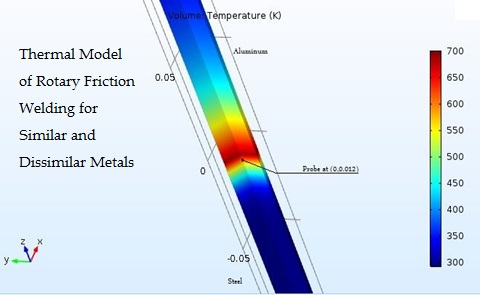
8]. Friction welding being a multi-physics phenomenon cannot be just expressed as a model of a single physical process. For this purpose, the modules of ‘solid mechanics’ and ‘heat transfer in solids’ were used. In solid mechanics, the contact pair was defined as a frictional contact with a static frictional coefficient of 0.61 between Aluminum and Steel [
9]. In heat transfer in solids, the process is to determine the ‘pair thermal contact’ and use the following equation, as used by Can et al. [
7] for calculation of the heat flux
.
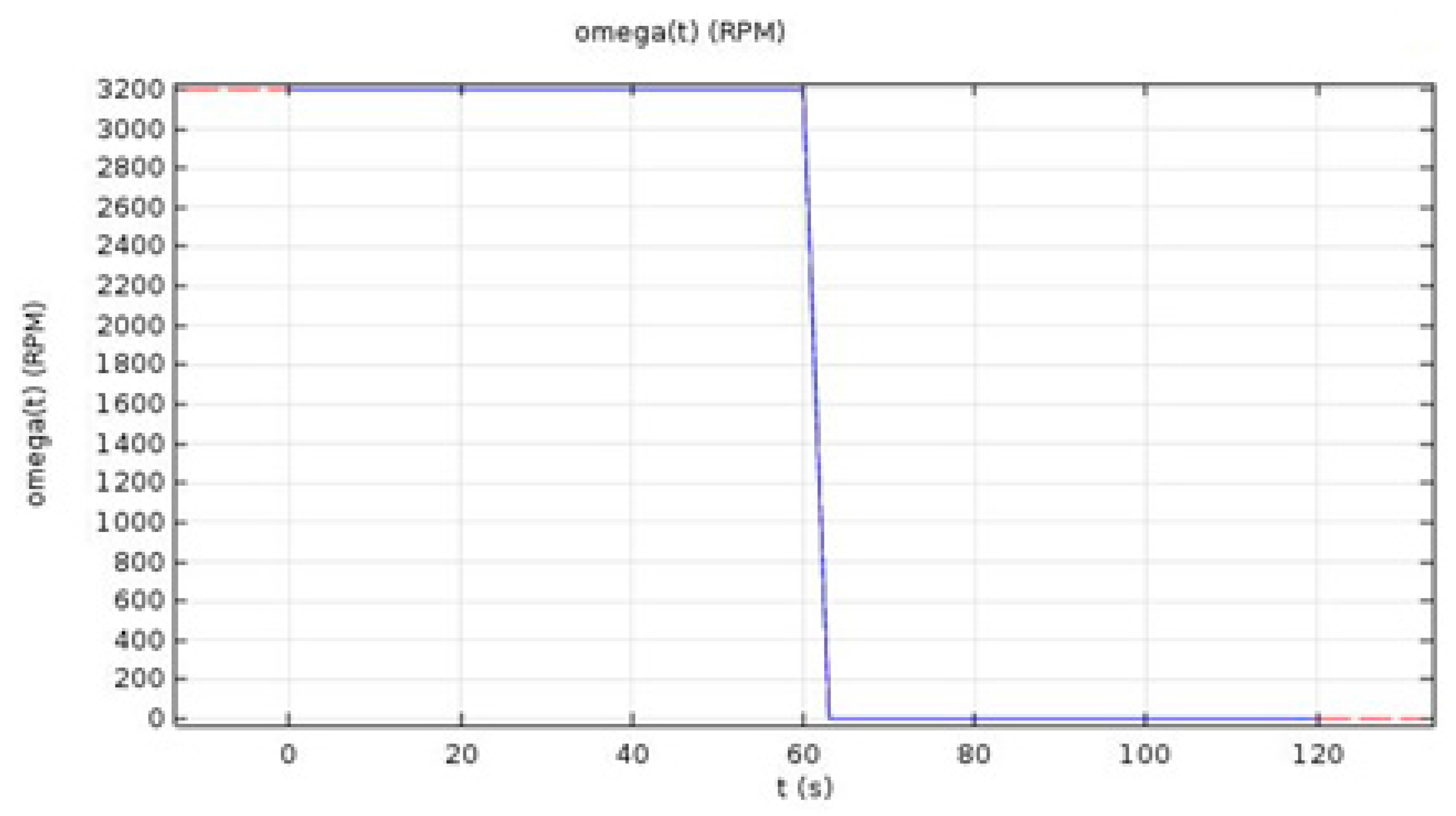
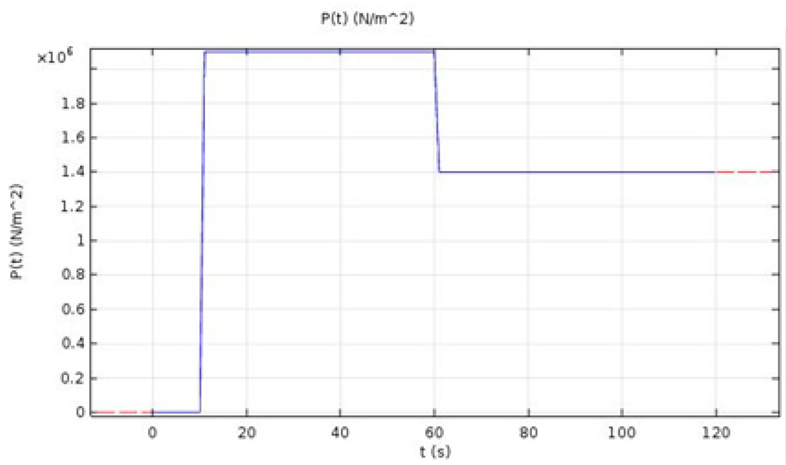
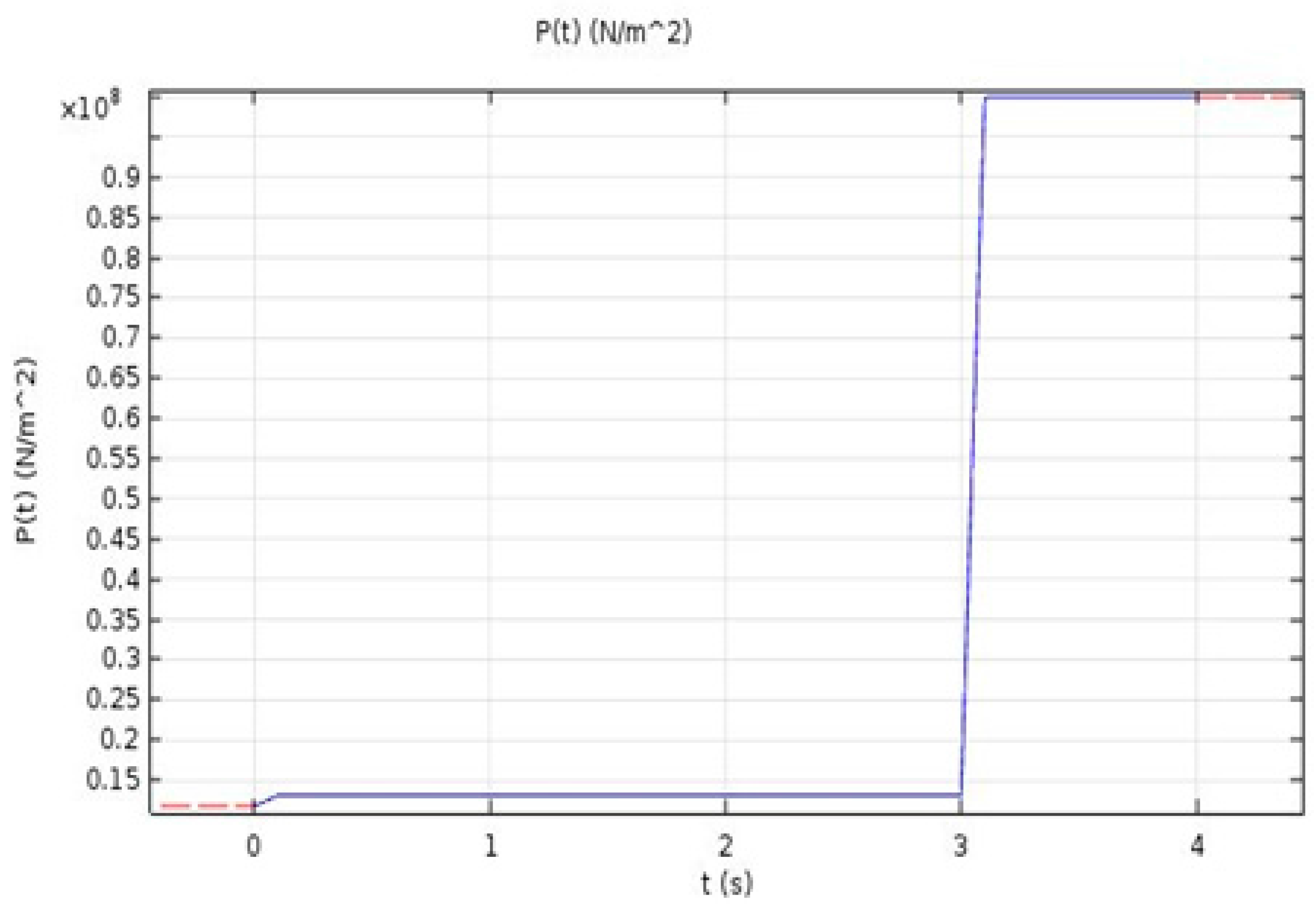
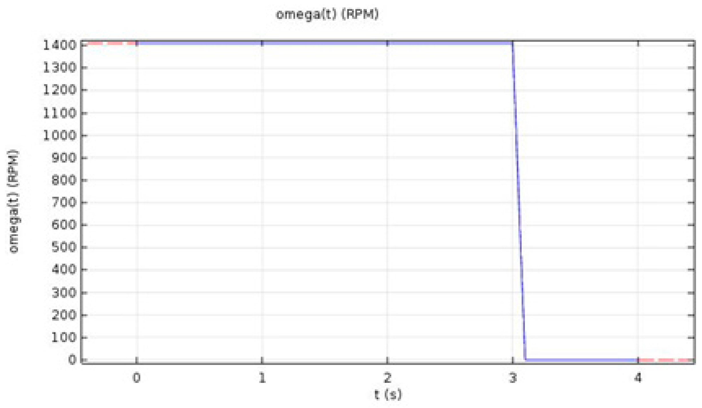
In this equation, is the rotational speed of the work-piece, P is the pressure being applied, and r is the radius of the work-piece.
The ‘heat transfer module’ in COMSOL uses the ‘apparent heat capacity method’ [
10] for the modeling of phase change phenomenon. In this method, an additional term is added to heat capacity i.e., ‘latent heat’. The heat transfer equation along with a convective term is as follows:
In this equation ρ is the density, Cp is the heat capacity, T is the temperature and k is the thermal conductivity.
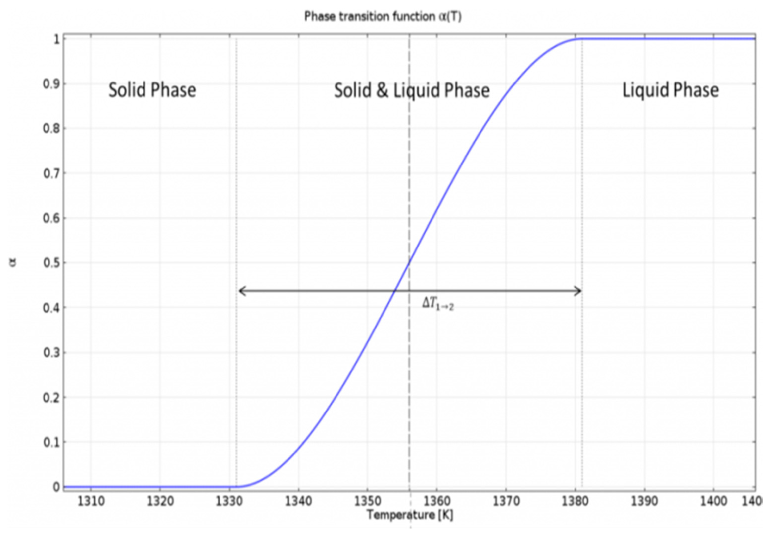
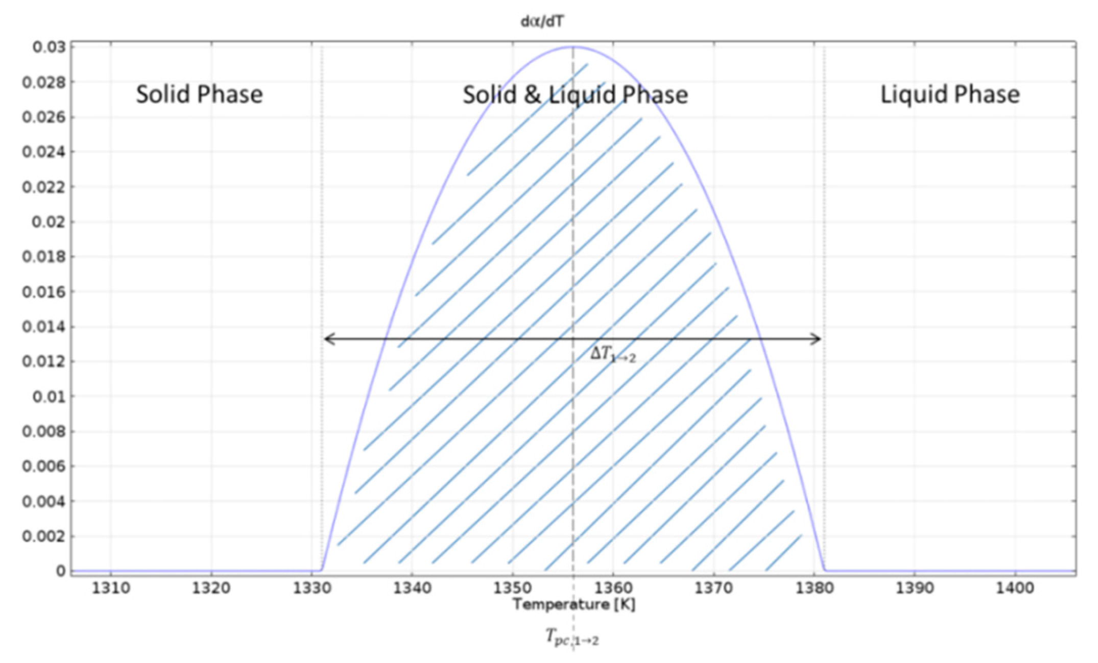
This ‘apparent heat capacity method’ uses a phase transition function
α(
T). During the implementation of the phase change, the interval (∆
T1→2) is to be defined, through which a smooth transition occurs. The material has mixed properties of liquid and solid forms in this interval, with its density ‘
ρ’ (kg/m
3) and thermal conductivity ‘
k’ (W/(m·K).
Figure 3 shows an example of the phase transition function for the phase change of iron [
11].
The transition function
α(
T) changes its value from 0 to 1 during this whole process of transition., namely
α(
T) = 0 for pure solid and for pure liquid
α(
T) = 1. In COMSOL, the material properties for solid and liquid phases are defined separately, but during the phase change, an equation depending on the transition function is used to find the combined properties for the transition phase. For the phase change, heat capacity ‘
Cp’ is given in Equation (3); wherein, ‘
α’ is the ‘linear thermal expansion coefficient’ (°K
−1) and ‘
T’ is the ‘temperature’ in (°K) [
12]:
The same process is used for finding other temperature dependent parameters, such as density and thermal conductivity. The equation caters for the change of properties during the phase transition. When ‘apparent heat capacity method’ is used, an additional term for ‘latent heat’ is added to the Equation (3).
In Equation (4),
L1→2 represents the latent heat from Phase 1 to Phase 2. The integration of this function during the interval ∆
T1→2 gives the total value of 1, and its multiplication with
L1→2 gives the amount of ‘latent heat’, which is released over ∆
T1→2 as shown in
Figure 4 below.

 ,
, 


