Future Projection with an Extreme-Learning Machine and Support Vector Regression of Reference Evapotranspiration in a Mountainous Inland Watershed in North-West China

Abstract

This study aims to project future variability of reference evapotranspiration (ET₀) using artificial intelligence methods, constructed with an extreme-learning machine (ELM) and support vector regression (SVR) in a mountainous inland watershed in north-west China. Eight global climate model (GCM) outputs retrieved from the Coupled Model Inter-comparison Project Phase 5 (CMIP5) were employed to downscale monthly ET₀ for the historical period 1960–2005 as a validation approach and for the future period 2010–2099 as a projection of ET₀ under the Representative Concentration Pathway (RCP) 4.5 and 8.5 scenarios. The following conclusions can be drawn: the ELM and SVR methods demonstrate a very good performance in estimating Food and Agriculture Organization (FAO)-56 Penman–Monteith ET₀. Variation in future ET₀ mainly occurs in the spring and autumn seasons, while the summer and winter ET₀ changes are moderately small. Annually, the ET₀ values were shown to increase at a rate of approximately 7.5 mm, 7.5 mm, 0.0 mm (8.2 mm, 15.0 mm, 15.0 mm) decade⁻¹, respectively, for the near-term projection (2010–2039), mid-term projection (2040–2069), and long-term projection (2070–2099) under the RCP4.5 (RCP8.5) scenario. Compared to the historical period, the relative changes in ET₀ were found to be approximately 2%, 5% and 6% (2%, 7% and 13%), during the near, mid- and long-term periods, respectively, under the RCP4.5 (RCP8.5) warming scenarios. In accordance with the analyses, we aver that the opportunity to downscale monthly ET₀ with artificial intelligence is useful in practice for water-management policies.

1. Introduction

Reference evapotranspiration (ET₀) is a significant parameter for agriculture, ecosystems and hydrological modeling [1,2]. ET₀ is one of the most important indicators of global climate change and hydrological regime changes [3]. Therefore, the estimation and projection of trends in ET₀ can be very important for water-resource management, precision agriculture, irrigation planning, and hydrological modeling studies [4,5,6]. In the last few decades, many different models, including water budget-based, mass transfer-based, temperature-based, radiation-based and combination approaches, have been used to estimate ET₀ [7,8,9]. Based on a significantly large number of existing research studies, the FAO-56 Penman–Monteith (PM) equation is considered to be the most precise and widely used approach for estimating ET₀ and for providing the validation standard for the other predictive models [3,10,11,12,13]. Many studies have regarded the ET₀ values estimated by the FAO-56 PM method as reference values for the other methods [14,15].

Other than the utilization of traditional ET₀ estimation methods, artificial intelligence (AI) based approaches have also been tested to estimate ET₀, as well as other real-life case studies [16,17,18,19,20,21]. For instance, Kumar et al. [22] first investigated the ability of AI-based models in ET₀ estimation, where artificial neural network (ANN) models were validated for this purpose. A number of other researchers have also paid considerable attention to the use of AI-based methods in estimating ET₀ where ANN, adaptive neuro-fuzzy inference system (ANFIS), support vector regression (SVR), general neuro-fuzzy models, gene-expression programming, M5 Model Tree (M5Tree), extreme-learning machines (ELM), and so on, have been applied [4,5,23,24,25,26,27,28,29,30,31,32,33]. Among these AI-based methods, the SVR model is considered to be one of the novel models to have been widely applied in ET₀ estimation studies. Wen et al. [34] evaluated the potential utility of SVR to model the daily ET₀ with limited climatic data in an extremely arid region. The results indicated that the SVR-based ET₀ was in good agreement with the FAO-56 PM based ET₀ calculations. Furthermore, the use of SVR, ANFIS-, regression- and climate-based models for ET₀ estimation in a semi-arid highland environment were also investigated by Tabari et al. [35], whose results revealed that the SVR model was considerably better than those attained by applying the regression- and climate-based models. In another study, the results from Yin et al. [36] obtained in a semi-arid mountain area showed that the SVR model was much better than the ANN model applied for estimating the daily ET₀ data. In fact, Kisi [37] found that the least square SVR models were considerably superior to the ANN models for the estimation of ET₀ data. Given the superiority of the SVR model in estimating ET₀, this method has been proven to possess good stability with relatively high prediction accuracy in many locations.

Recently, an extreme-learning machine (ELM), regarded as an AI-based fast and efficient learning technique, has been introduced and tested in many different fields of research [38,39,40,41,42,43,44,45,46,47]. A review of the applications and trends of studies using the ELM model has been performed by Huang et al. [48]. In respect of the use of this method for an estimation of evapotranspiration, Abdullah et al. [5] first investigated the efficiency of the ELM method for the prediction of FAO-56 PM ET₀ data for three meteorological stations in Iraq, and the results proved that the ELM model was highly efficient in ET₀ estimation. Then, Gocic et al. [49] applied the ELM model to estimate monthly ET₀ for two weather stations in Serbia using data for a 31-year period, and the ELM-based ET₀ data was compared with the results of the Hargreaves, Priestley–Taylor, and Turc equations. Evidently, the ELM model was found to be a better predictive tool than the other models considered for modeling monthly ET₀ data. Although the ELM model is a relatively new AI-based method used for ET₀ estimation, the model has been used rapidly in different locations and has proved to be an efficient and satisfactory tool for predicting ET₀.

Data from the Intergovernmental Panel on Climate Change (IPCC) repositories show that global average air temperature has increased by 0.85 °C from 1880 to 2012, and would further rise by 1.5 °C by the end of the 21st century [50,51]. If so, this can directly or indirectly affect other climatic variables because of their links to atmospheric circulation [52]. It is notable that, as a result of climatic change, ET₀ has increased or decreased in different regions of the world [52,53,54,55,56]. Considering the uncertainty as to how the ET₀ might change and its complex role in moderating climates in different regions, the projected future trends in ET₀ under the background of climate change continues to receive significant attention.

Future ET₀ projections can be performed using physically-based models and statistical methods (e.g., Penman–Monteith equations) or by AI-based models (e.g., ANN, SVR and ELM models) where the output climatic variables from global climate models (GCMs) and local-scale, nested systems such as regional climate models (RCMs) are adopted. Li et al. [57] examined the present and future characteristics of ET₀ on the Loess Plateau of China based on historical weather data in order to downscale HadCM3 (Hadley Centre Coupled Model, version 3) outputs. That study showed that the ET₀ values increased significantly during the 1961–2009 period, whereas the HadCM3 projections showed a continuous increase in ET₀ values into the 21st century. The future ET₀ projections on the Loess Plateau in the study of Gao et al. [58], using CMIP5 data, also demonstrated increasing trends during the 2001–2050 period. The future ET₀ on the Loess Plateau was also investigated by the study of Peng et al. [59] where the average annual ET₀ was shown to increase by approximately 12.7–23.9% from 1961 to 1990 towards the end of the 21st century. Xing et al. [13] conducted an investigation on present and future changes (i.e., 2011–2099) in ET₀ in the Haihe River Basin of China through the outputs of climatic variables extracted from the Phase 3 of the Coupled Model Intercomparison Project (CMIP3). Concluding that the future projection of ET₀ is significant in assessing the hydrological regime change impacted by climate change, the study of Wang et al. [3] selected different approaches to investigate the differences of future ET₀ response to climate change in accordance with HadCM3 outputs for the Hanjiang River Basin. The results showed that the water surplus exhibited a likely decreasing trend in the period 2011–2099. Kundu et al. [60] estimated the future change (2011–2099) trends of ET₀ in central India by downscaling HadCM3 output data.

In accordance with the reviews, it is evident that future ET₀ changes has been projected for many regions of the world based on simulated outputs of GCM. However, current studies have mainly been based on conventional (i.e., statistical) methods and models (e.g., the Hargreaves equation). AI-based models that have the ability to integrate historical knowledge (i.e., changes in ET₀) with GCM-simulated data in order to perform modeling have seldom been used to estimate future ET₀ values. Several studies have applied downscaling techniques based on artificial neural networks (ANN), multiple linear regressions and other statistical models, owing to their ability to capture non-linear relationships between ground and GCM-based predictors in respect of the predictands, such as rainfall, winds, cloud cover, streamflow and temperature (e.g., [61,62,63]).

In this paper, we have adopted two well-established AI techniques, the support vector regression (SVR) and extreme-learning machine (ELM) algorithms, considering their popularity as robust tools applied in the area of predictive modeling. Notably, the SVR model is a statistical model based in theory that utilizes the regularization framework, presenting advancement over conventional artificial neural network models; whereas the ELM model is a fast and efficient neuro-computational approach offering an improvement in its design and universal approximation capability compared to conventional ANN models. The ELM model was shown to perform more accurately than the SVR and ANN models for drought studies [46] and the simulation of streamflow [47]. To the authors’ best knowledge, the SVR and ELM models have not been fully explored for the future projection of ET₀. Serious consideration should be given to the fact that most of the future ET₀ projections have been based on the outputs of single-simulation climate models (e.g., HadCM3) that have some degree of uncertainty due to the models’ internal variability and fidelity. Uncertainties are likely to degrade a model’s overall predictive skill [64]. It is thus desirable that climate modelers and climate policy-makers assess more quantitatively a model’s fidelity with respect to observed records, addressed by means of multi-model ensemble projections, in order to reduce uncertainties in the downscaled variables.

Considering the aforementioned review of literature, this study employs two well-established AI-based models comprising ELM and SVR algorithms to project future changes in ET₀ in an inland mountainous watershed region of China in which data from GCM outputs of CMIP5 are utilized. In order to reduce the uncertainties of single-simulation GCM models, in this paper we have selected eight-model ensemble projections (from CMIP5) to analyze the overall future variability of ET₀ in northwest of China. The FAO-56 PM based ET₀ has been chosen as the verification standard for the downscaled data, which is meaningful for agricultural applications. The rest of the paper is structured as follows. Section 2 details the materials and methods, including a description of the study area, datasets, methodologies, model development and performance-evaluation measures; Section 3 gives the details of the results; Section 4 includes the discussion; and Section 4 lists the conclusions of this research.

2. Materials and Methods

2.1. Study Area

The Heihe is a famous inland river in China, located in the central part of the Hexi Corridor. In this study, we selected as the study area the headwater region (Yingluoxia Watershed) of the Heihe River (Figure 1) which is located on the north slope of Qilian Mountain covering an area of 10,018 km² lying between 99° to 101° E and 38° to 39° N. About 90% of the water resources of the Heihe River are generated from the Yingluoxia (YLX) Watershed. The water resources from the YLX Watershed supply more than 1.3 million people in China, support about 266,000 ha of irrigated agricultural land midstream and downstream, and also play a major role in maintaining the stability of the natural ecosystem. Considering these factors, the YLX Watershed is a very important inland area that has attracted much research attention in China. The climate of the watershed is characterized by hot and wet conditions in summer and cold and dry conditions in winter. The annual precipitation data shows a decrease in rainfall from the east to the west of the region, and an increase from approximately 200 mm to 700 mm with an increase in altitude. Detailed descriptions of the YLX Watershed can be found in previous studies of Yin et al. [65] and Cheng et al. [66].

2.2. Datasets

In this study, we have adopted two different datasets, including the observed historical weather data and the simulated global climate model (GCM) outputs, in order to calculate the ET₀ for the YLX Watershed region for the historical period 1961–2005 and the future period 2010–2099, respectively. The historical weather data including the daily maximum, minimum and mean temperature, relative humidity (%), precipitation (mm), wind speed (m/s), atmospheric pressure (hPa) and sunlight duration (h) at 4 weather stations in and around the YLX Watershed were downloaded from the China Meteorological Administration (http://data.cma.cn/) for the period 1961–2005. The simulated historical daily data in the same period for a total of 8 GCMs were acquired from the Coupled Model Intercomparison Project Phase 5 (CMIP5) project. The projected future daily data (e.g., daily maximum, minimum and mean temperature, daily relative humidity, wind speed, atmospheric pressure, etc.) were acquired for the period 2010–2099 for two distinct scenarios based on the Representative Concentration Pathways (RCP4.5 and 8.5) extracted from the simulations of the 8 GCMs.

Table 1. Summary of global climate models from CMIP5 simulation set.

Id	Model	Centre Acronym(s)/Country	Scenarios	Reference
1	ACCESS1.0	CSIRO-BOM/Australia	Historical; RCP4.5; RCP8.5	[67]
2	ACCESS1.3	CSIRO-BOM/Australia	Historical; RCP4.5; RCP8.5	[67]
3	BCC-CSM1.1(m)	BCC/China	Historical; RCP4.5; RCP8.5	[68]
4	CNRM-CM5	CNRM-CERFACS/France	Historical; RCP4.5; RCP8.5	[69]
5	HadGEM2-CC	MOHC/UK	Historical; RCP4.5; RCP8.5	[70]
6	HadGEM2-ES	MOHC/UK	Historical; RCP4.5; RCP8.5	[70]
7	MIROC5	MIROC/Japan	Historical; RCP4.5; RCP8.5	[71]
8	MRI-CGCM3	MRI/Japan	Historical; RCP4.5; RCP8.5	[72]

shows the details of the 8 GCM outputs.

In order to downscale ET₀ for the mountainous inland watershed region in north-west China, in this study we have employed two different AI-based techniques where the ELM and SVR algorithms were used to model ET₀ for the historical period (1961–2005) and the future period (2010–2099). In this regard, during the historical simulation period, the observed and simulated historical datasets were partitioned into two distinct phases; with the first 30 years’ of data (i.e., 1961–1990) utilized as a training set and the remaining 15 years’ data (i.e., 1991–2005) utilized as a testing set. The projected future datasets were also divided into three segments of 30-year forecast horizons, which were denoted as: 2010–2039, 2040–2069, 2070–2099 to represent the climate change of the near-term, mid-term and long-term periods, respectively.

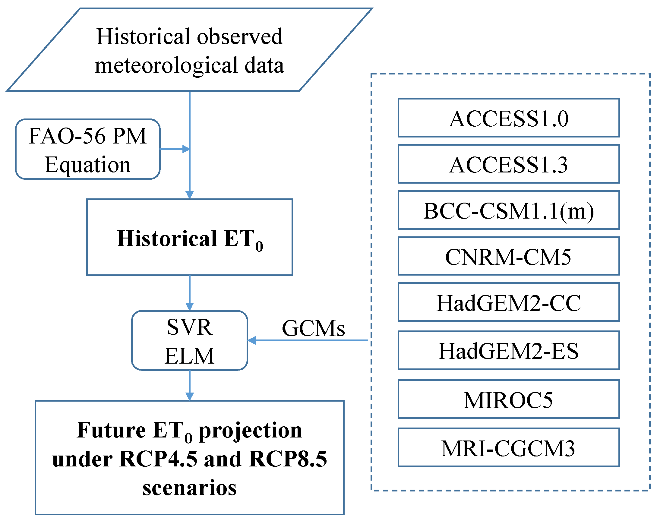
2.3. Computational Methodology

2.3.1. FAO-56 Penman–Monteith Equation

ET₀ values computed by the FAO-56 Penman–Monteith equation were used in this study to evaluate the performance of the other prediction methods. Mathematically, the Penman–Monteith equation is expressed as follows:

$$E{T}_0=\frac{0.408\Delta \left(R_n-G\right)+\gamma \frac{900}{T_{mean}+273}{U}_2\left(e_s-e_a\right)}{\Delta +\gamma \left(1+0.34U_2\right)}$$

(1)

where ET₀ is the reference evapotranspiration (mm day⁻¹); Δ is the slope of the saturation vapor pressure–temperature curve (kPa °C⁻¹); R_n is the net radiation (MJ m⁻² day⁻¹); G is the soil heat flux (MJ m² day⁻¹); γ is the psychrometric constant (kPa °C⁻¹); T_mean is the average daily air temperature at 2 m (°C); U₂ is the mean daily wind speed at 2 m (m s⁻¹); e_s is the saturation vapor pressure (kPa); and e_a is the actual vapor pressure (kPa). The computations from all data required the calculation of the ET₀ following the method and procedures outlined in Chapter 3 of the FAO-56 manual [73].

2.3.2. Extreme-Learning Machine

The extreme-learning machine (ELM) as an AI-based method was first introduced by Huang et al. [38,74]. The learning speed of the ELM model is relatively faster than the conventional feed-forward network without the need for too much human intervention, but this model is able to offer better generalization performance than the conventional ANN model [42,46,47,75]. ELM is based on single-layer feed-forward neural networks (SLFNNs) architecture [5] where there are 3 layers, including the input layer, hidden layer, and output layer. An important distinction and advantage of ELM as an improved version of the ANN model is that the hidden layer does not need to be tuned iteratively. Hence, the ELM model is able randomly to screen the input weights, and then analytically determine the output weights (e.g., feature-analyzed property) of the SLFNNs. Detailed descriptions of the ELM can be found in Huang et al. [74], Gocic et al. [49], Abdullah et al. [5], and Patil and Deka [33].

For i = 1, 2, …, N, the SLFN with L hidden neurons is expressed as:

$${\psi }_L(x)={\displaystyle \sum _{i=1}^{i=L}}{h}_i\left(x\right){\beta }_i=h(x)\beta$$

(2)

where, $\beta$ ${\left[{\beta }_1,{\beta }_2,\cdots ,{\beta }_L\right]}^T$ is the output weight matrix computed between the hidden and the output neurons; $h\left(x\right)$ $\left[h_1,h_2,\cdots ,h_L\right]$ is the hidden neuron outputs representing the randomized hidden features of predictor X_i; and $h_i\left(x\right)$ is the ith hidden neuron, given as:

$$h_i\left(\mathbf{x}\right)=\vartheta \left({\mathbf{a}}_i,b_i,\mathrm{{\rm X}}\right)and{\mathbf{a}}_i\in R^d,b_i\in R$$

(3)

The non-linear piecewise-continuous hidden layer activation function $h_i\left(x\right)$ is defined using hidden neuron parameters (a, b) and must satisfy the approximation theorem, $\mathsf{\vartheta }\left(a_i,b_i,\mathit{X}\right)$. The model’s approximation error is minimized when solving for weights connecting the hidden and output layer (β) using a least square method:

$$\underset{\beta \in R^{L\times m}}{\min }{\Vert \mathbf{H}\beta -\mathbf{T}\Vert }^2$$

(4)

here, $\Vert \Vert$ is the Frobenius norm, and

H is the hidden layer output matrix, given as:

$$\mathbf{H}=\left[\begin{array}{c}g\left(x_1\right)\\ ⋮\\ g\left(x_N\right)\end{array}\right]=\left[\begin{array}{ccc}{g}_1\left(a_1{x}_1+b_1\right)& \cdots & g_L\left(a_L{x}_1+b_L\right)\\ ⋮& \cdots & ⋮\\ g_1\left(a_N{x}_N+b_1\right)& \cdots & g_L\left(a_L{x}_N+b_L\right)\end{array}\right]$$

(5)

T is the target matrix, drawn from the training dataset, and given as:

$$\mathbf{T}=\left[\begin{array}{c}{\mathbf{t}}_1^T\\ ⋮\\ {\mathbf{t}}_N^T\end{array}\right]=\left[\begin{array}{c}{t}_{11}\\ ⋮\\ t_{N1}\end{array}\begin{array}{c}\\ \\ \end{array}\begin{array}{c}\cdots \\ \\ \cdots \end{array}\begin{array}{c}\\ \\ \end{array}\begin{array}{c}{t}_{1m}\\ ⋮\\ t_{Nm}\end{array}\right]$$

(6)

An optimal solution is then determined by solving a system of linear equations:

$${\beta }^{*}={\mathbf{H}}^{+}\mathbf{T}$$

(7)

and H⁺ is the Moore–Penrose generalized inverse function (+).

2.3.3. Support Vector Regression

Support vector regression (SVR) is an effective forecasting tool developed for solving regression problems by Vapnik [76]. SVR is a next-generation statistical learning method where data features can be learned from high-dimensional, and a small number of, training data [77]. SVR is used to describe a regression-based modeling process where the following linear estimation function could be employed:

$$f\left(x\right)=\omega \cdot \phi \left(x\right)+b$$

(8)

where ω is weight vector; b is a constant; and $\phi \left(x\right)$ denotes a mapping function in the feature space. The coefficients ω and b can be estimated by minimizing:

$$R_{reg}\left(f\right)=C\frac{1}{N}{\displaystyle {\sum }_{i=1}^N{L}_{\epsilon }\left(f\left(x_i\right),y_i\right)}+\frac{1}{2}{\Vert w\Vert }^2$$

(9)

$$L_{\epsilon }\left(f\left(x\right)-y\right)=\{\begin{array}{ll}\left|f\left(x\right)-y\right|-\epsilon & for\left|f\left(x\right)-y\right|\ge \epsilon \\ 0& otherwise\end{array}$$

(10)

where both C and ε are prescribed parameters. The term $L_{\epsilon }\left(f\left(x_i\right),y_i\right)$ is called the ε-intensive loss function. This function indicates that errors below ε are not penalized. The term $C\frac{1}{N}{\displaystyle {\sum }_{i=1}^N{L}_{\epsilon }\left(f\left(x_i\right),y_i\right)}$ is the empirical error. The term $\frac{1}{2}{\Vert w\Vert }^2$ measures the smoothness of the function. C evaluates the trade-off between the empirical risk and the smoothness of the model. A Largrange multiplier and optimality constraints are used, so a nonlinear regression function is obtained using the following expression:

$$f\left(x\right)={\displaystyle {\sum }_{i=1}^l\left({\alpha }_i-{\alpha }_i^{*}\right)k\left(x_i,x\right)}+b$$

(11)

where α_i and α_i^* are the introduced Lagrange multipliers, and k(x_i, x) is kernel function.

2.3.4. Model Development

In this study, we have employ ELM and SVR models to establish the relationship between the estimated ET₀ by the FAO-56 PM method with the historical observed meteorological variables and the GCM output variables. Figure 2 shows a schematic diagram for future ET₀ projection. First, we estimated ET₀ by using historically observed variables. Then, we used the historical ET₀ as target to directly downscale the GCM outputs by using the ELM and SVR. Thus, we divided the 45-year data set representing the current climate (1961–2005) into two sub-period datasets. The first 30 years of data (1961–1990) were used for developing and calibration the regression-based AI models; while the remaining 15 years of data (1991–2005) were used to validate the models.

To investigate the variability of future ET₀, the Sen Slope method and Mann–Kendall (M–K) Test [78] were employed.

2.3.5. Model Goodness-of-Fit Criteria

To evaluate the effectiveness of the downscaling approaches, four statistical score metrics, including the coefficient of correlation (R), mean absolute relative error (MAE), root mean square error (RMSE) and Nash–Sutcliffe efficiency (NSE) [79,80] were selected. In fact, the R value, which is expressed as the degree of correlation between the FAO-56 PM based ET₀ and the downscaled ET₀ by the SVR and ELM models, respectively, measures the covariance in the two datasets. The MAE and RMSE provide different types of information about the estimation abilities of the AI-based models, whereby the RMSE (mm/month) is able to evaluate the goodness-of-fit relevant to the peak values and the MAE (mm/month) is able to generate the performance index of modeled ET₀ and the distribution of the modeling errors. It should be noted that both of these metrics are required in the mode evaluation phase since they can provide complementary information about the accuracy of modeled ET₀. In accordance with the literature [79], the RMSE is a more appropriate metric when the error distribution is found to be Gaussian, whereas RMSE (due its squaring effects) should be used to assess the errors that are not normally distributed. Mathematically, the R value is expressed as:

$$R=\frac{{\displaystyle {\sum }_{i=1}^N\left(E{T}_{0-\mathbf{PM},i}-\overline{E{T}_{0-\mathbf{PM},i}}\right)\left(E{T}_{0-\mathbf{AI},i}-\overline{E{T}_{0-\mathbf{AI},i}}\right)}}{\sqrt{{\displaystyle {\sum }_{i=1}^N{\left(E{T}_{0-\mathbf{PM},i}-\overline{E{T}_{0-\mathbf{PM},i}}\right)}^2{\displaystyle {\sum }_{i=1}^N{\left(E{T}_{0-\mathbf{AI},i}-\overline{E{T}_{0-\mathbf{AI},i}}\right)}^2}}}}$$

(12)

The MAE value is expressed as:

$$MAE=\frac{1}{N}{\displaystyle {\sum }_{i=1}^N\left|\left(E{T}_{0-\mathbf{AI},i}-E{T}_{0-\mathbf{PM},i}\right)\right|}$$

(13)

The RMSE value can be calculated as:

$$RMSE=\sqrt{\frac{1}{N}{\displaystyle {\sum }_{i=1}^N{\left(E{T}_{0-\mathbf{AI},i}-E{T}_{0-\mathbf{PM},i}\right)}^2}}$$

(14)

The NSE value can be calculated as:

$$NSE=1-\left[\frac{{\displaystyle {\sum }_{i=1}^N{\left(E{T}_{0-\mathbf{PM},i}-E{T}_{0-\mathbf{AI},i}\right)}^2}}{{\displaystyle {\sum }_{i=1}^N{\left(E{T}_{0-\mathbf{PM},i}-\overline{E{T}_{0-\mathbf{PM},i}}\right)}^2}}\right],\infty \le NSE\le 1$$

(15)

In the above equations, N is the number of input test samples; $E{T}_{0-\mathbf{PM}}$ and $E{T}_{0-\mathbf{AI}}$ are the FAO-56 PM ET₀ and modeled ith ET₀ value; and $\overline{E{T}_{0-\mathbf{PM}}}$ and $\overline{E{T}_{0-\mathbf{AI}}}$ are the average of the FAO-56 PM value and modeled value of the ET₀. The best performances for the SVR and ELM models are expected to yield R = 1, MAE = 0, RMSE = 0 and NSE = 1, respectively.

3. Results

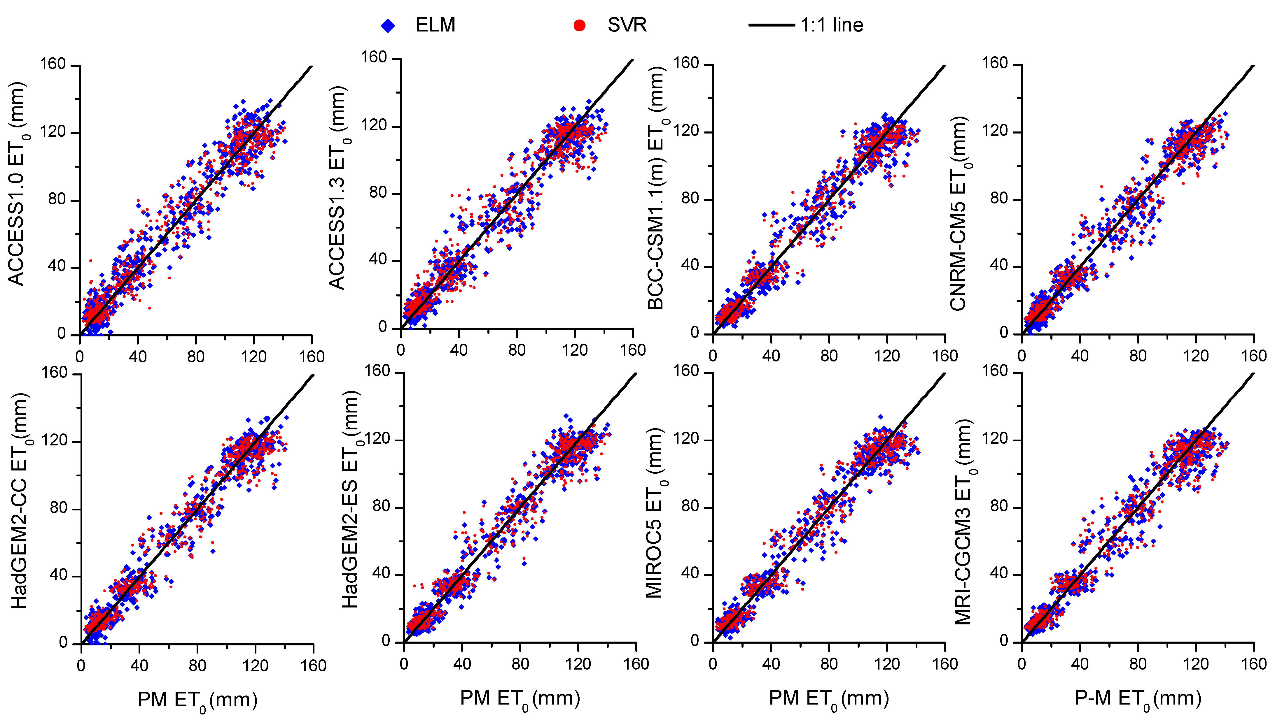
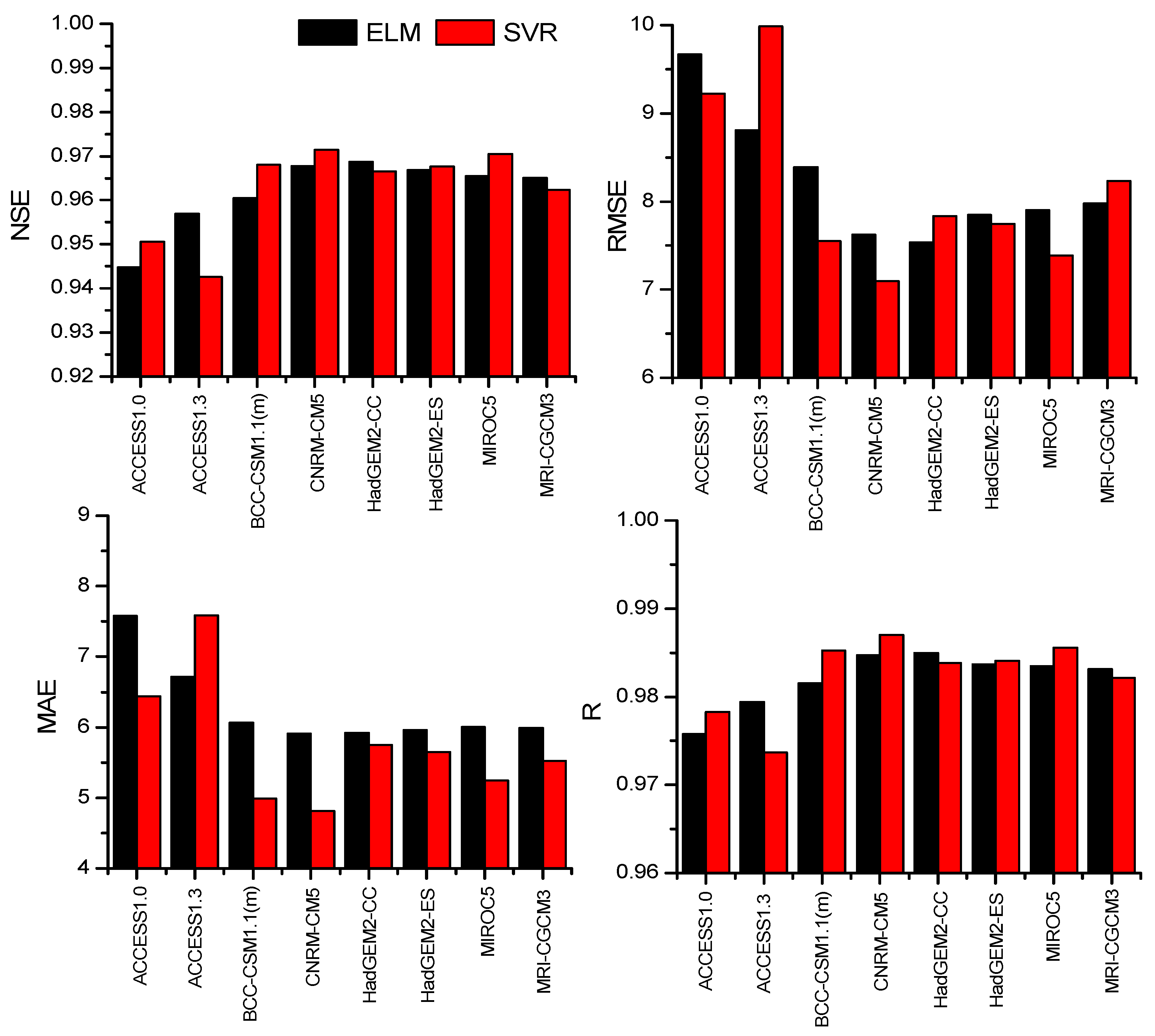
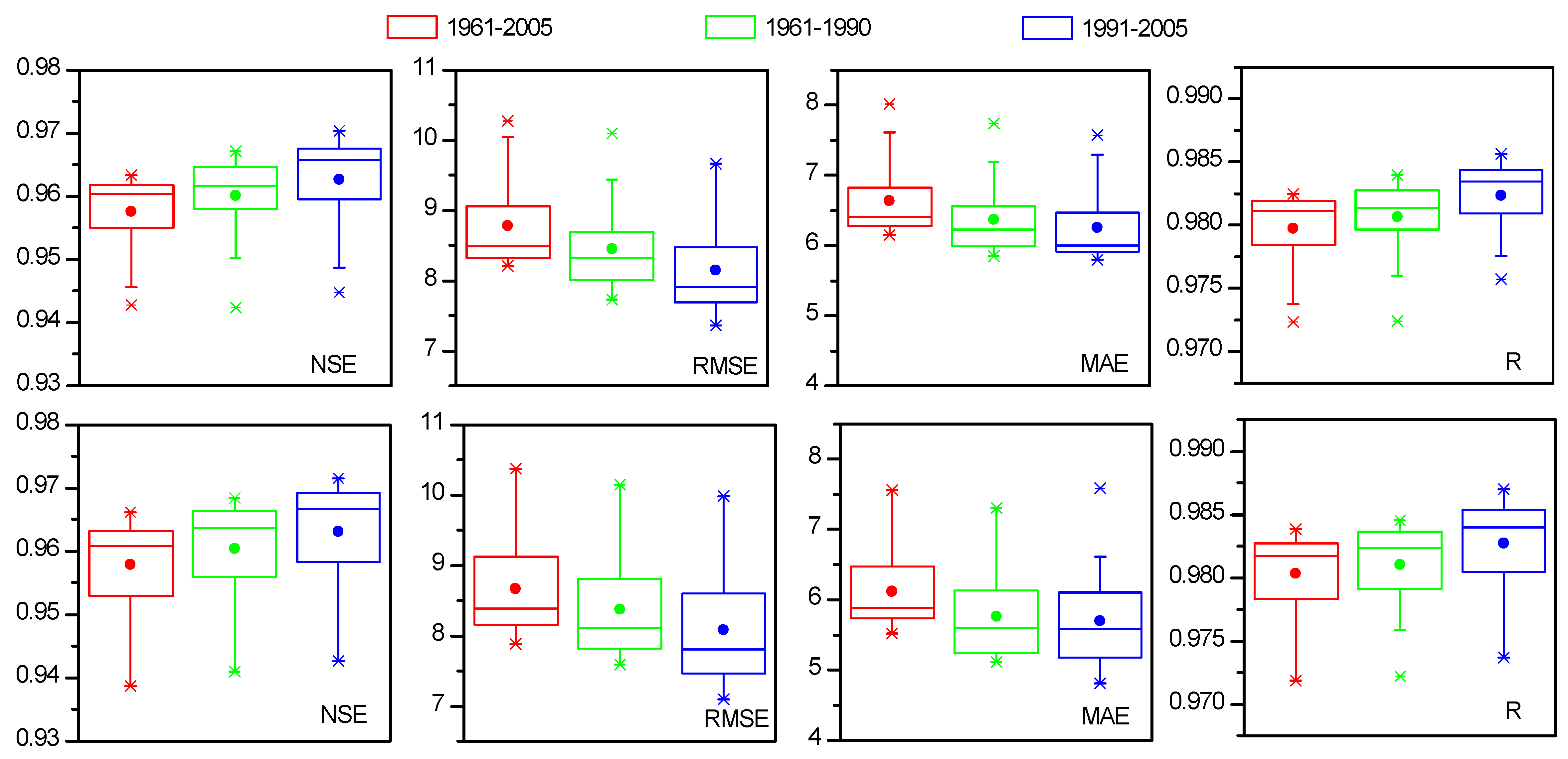
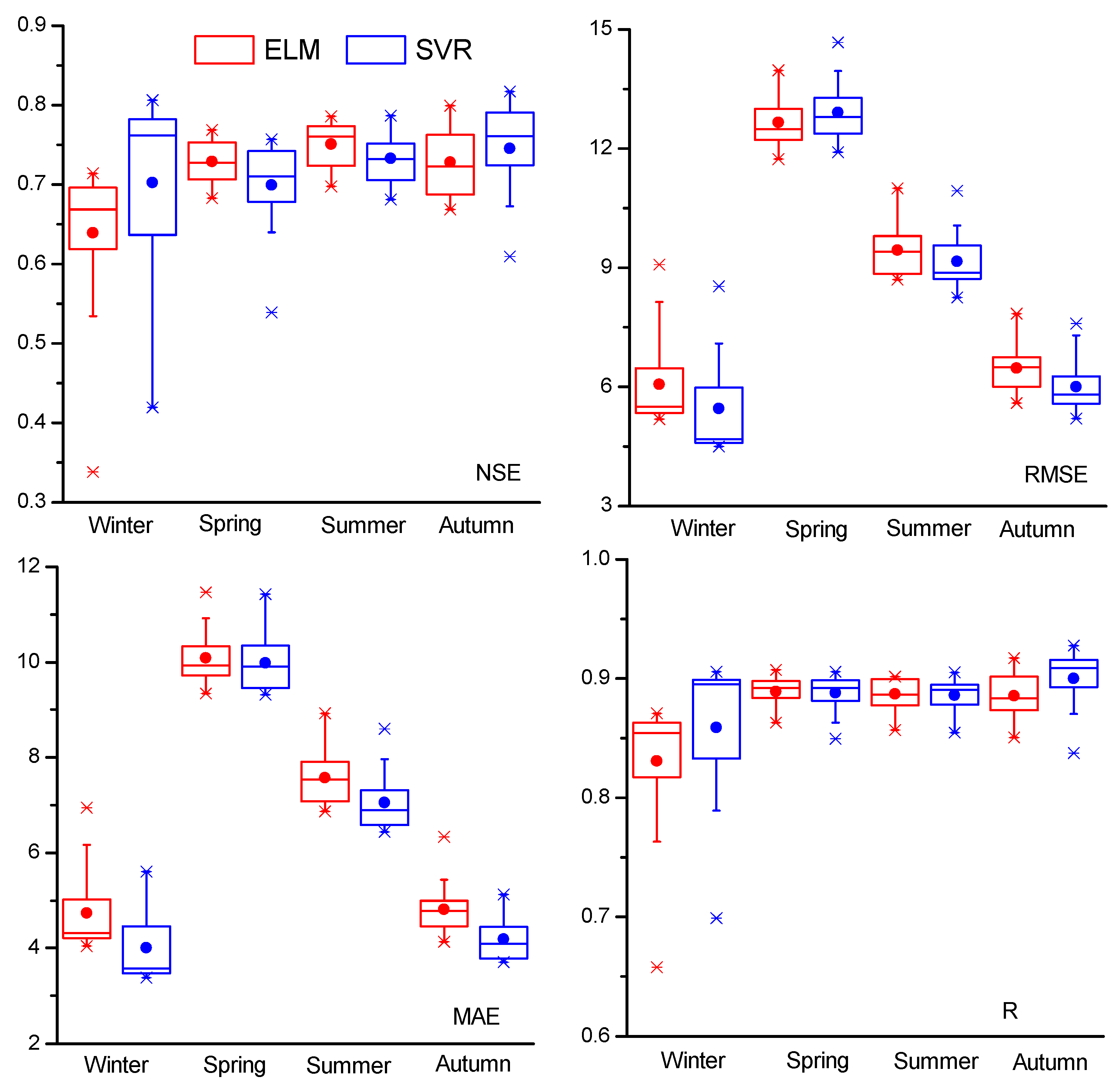
3.1. Model Verification and Comparison

The FAO-56 PM based ET₀ was calculated by deriving the historically observed meteorological variables (i.e., maximum and minimum air temperature, relative humidity, air pressure, sunlight duration and wind speed at 2 m height) for the period 1961 to 2005. The eight selected GCM outputs were extracted to compute ET₀ using ELM and SVR-based downscaling approaches. Figure 3 shows the correlation of these data with the FAO-56 PM based ET₀. Generally, it is evident that the GCM outputs-derived ET₀ exhibited a very good correlation in respect to the FAO-56 PM based ET₀ when the results for both ELM and SVR based methods were analyzed. This suggests that the GCM-derived ET₀ values are good representatives of the FAO-56 PM based ET₀ in this particular study region. The performance metrics for the GCM-derived ET₀ data in the validation period are shown in Figure 4. It is noteworthy that all of the ET₀ downscaled results revealed relatively good performances with the NSE values being greater than 0.94; the RMSE/MAE values being lower than 10 mm/month and 8 mm/month, respectively; and the R values being larger than 0.97. It is especially the case that the downscaled-derived ET₀ values from the BBC-CSM1.1(m), CNRM-CM5, HadGEM2-CC, HadGEM2-ES, MIROC5 and MRI-CGCM3 models registered acceptably high performance with NSE greater than 0.96; RMSE/MAE lower than 8 mm/month and 6 mm/month, respectively; and R values greater than 0.98. When the ELM and SVR model performances were compared, the results showed that at least five out of the eight GCM model outputs from the SVR-based calculations were better than those from the ELM-based calculations, with higher NSE and R values, and lower RMSE and MAE values. This indicates the SVR model had a better performance compared to the ELM model when used for downscaling the ET₀ data for the mountainous inland watershed region in north-west China.

Boxplots describing the four performance metrics for the ET₀ modelling by the ELM and SVR methods based on eight GCM outputs with different periods are shown in Figure 5. On the basis of these four performance metrics, the testing period (1991–2005) revealed a much better performance with a higher value of NSE and R, and a lower value of RMSE and MAE compared to those of the training period (1961–1990). It is important to note that when the entire period (1961–2005) was considered, the performance was even worse than that of the training period, indicating that the error in simulations increased with an increase in the modelling timespan. When compared in terms of the performances between the ELM and SVR approaches for downscaling the ET₀, it is observable that the median values of the NSE and R for the SVR model are considerably higher than those of the ELM model, and the RMSE and MAE values for the SVR model are much lower than those of the ELM model among the three different periods considered in this paper. This indicates that almost half of the GCM outputs-derived ET₀ calculations based on the SVR model are much better than those of the ELM model. In order to further verify this phenomenon, we have assessed the model performances at seasonal scales. Figure 6 shows the seasonal performance of the two AI-based methods, derived from the GCM outputs. Evidently, the four performance metrics for the SVR model appear to have largely increased relative to the ELM model in the winter and autumn seasons. This reveals that the SVR approach demonstrates a very good capacity to estimate the ET₀ data compared to the ELM model. In accordance with this, we can conclude that the SVR-calculated ET₀ simulations are more accurate than the ELM-based ET₀ simulations, which is attributable to the better ability of the SVR model to simulate this parameter in the winter and autumn seasons.

3.2. Evaluation of Future ET₀ Projections

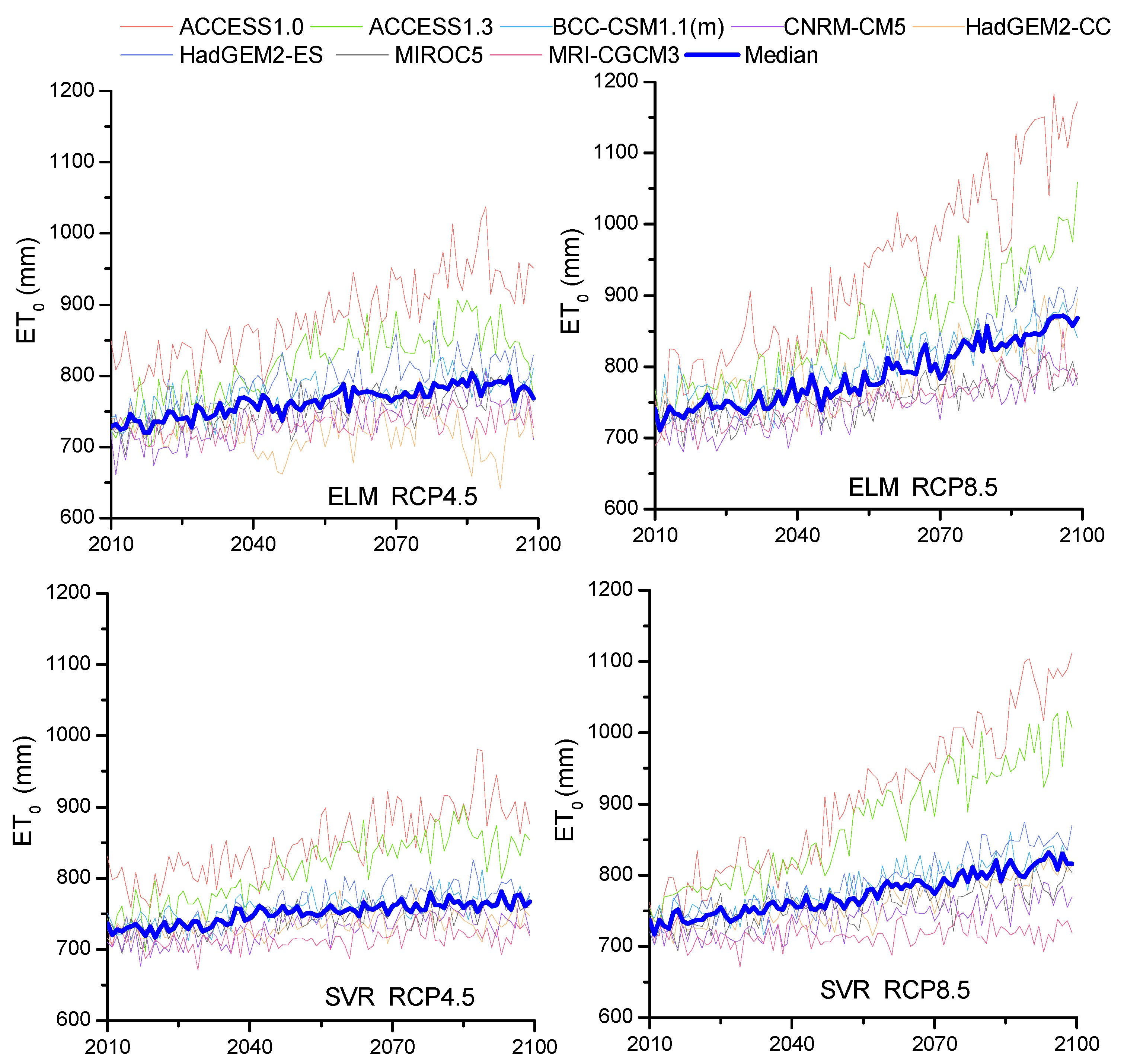
3.2.1. Annual Future ET₀

Figure 7 illustrates the future projections of ET₀ modelled by the ELM and SVR approaches, where a total of eight GCM outputs used as inputs for the AI-based models under RCP4.5 and RCP8.5 warming scenarios were investigated. In accordance with this result, there appears to be little difference between the performances of the ELM and SVR approaches for both scenarios. Notably, for the case of the RCP4.5 scenario, the ET₀ projections derived from the ACCESS1.0 model had the largest value, lying within the range of approximately 760–1100 mm for ELM and 750–970 mm for the SVR model, followed by the ACCESS1.3 model. Interestingly, the range appeared to be even broader for the case of the RCP8.5 warming scenario. The rest of the six GCM models registered very similar, and conservative, trends in the future under both warming scenarios. It should be noted that the ELM results revealed a larger variability than the SVR results. In order to eliminate the uncertainty caused by a single simulation model, we have adopted the median value of the eight GCM-derived ET₀ data to represent the ET₀ projections in the present study region. The range of the ET₀ data for the RCP4.5 is found to be approximately 720–760 mm and for the RCP8.5 warming scenario approximately 725–810 mm.

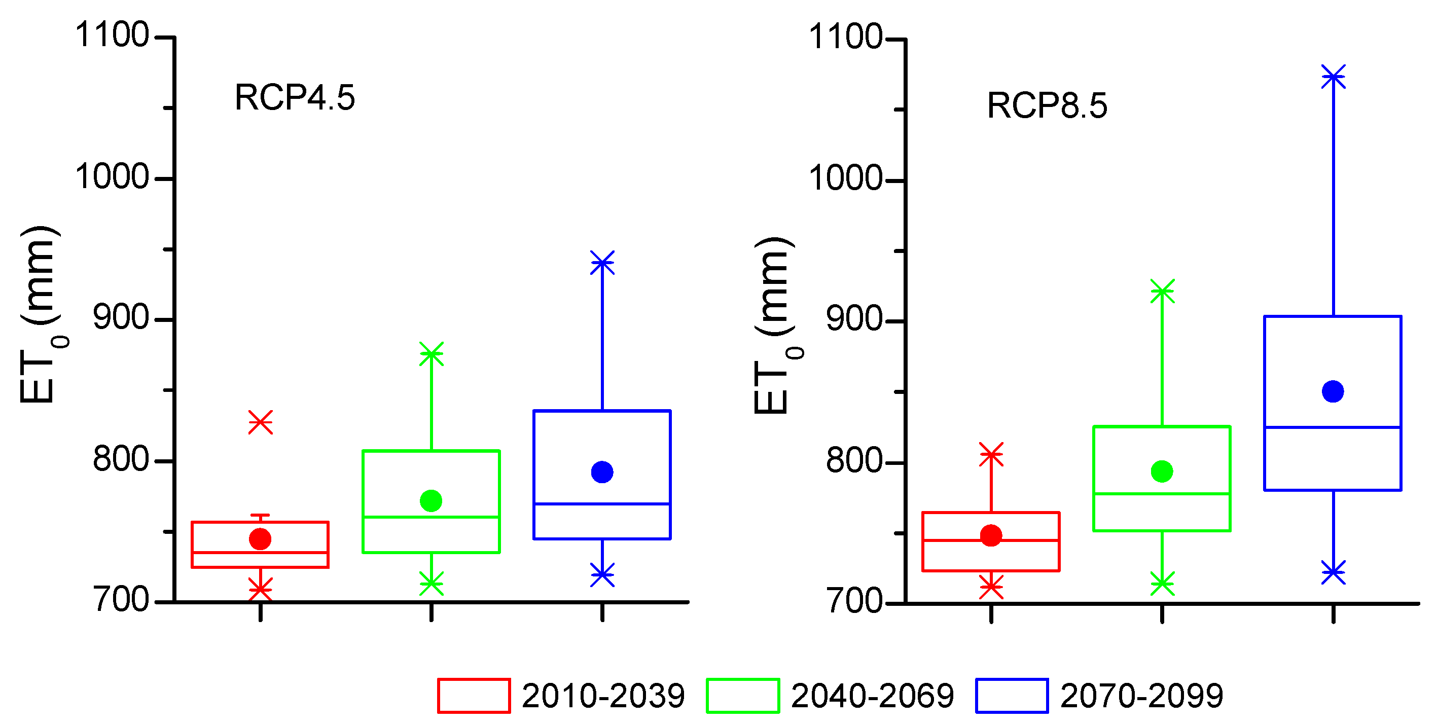
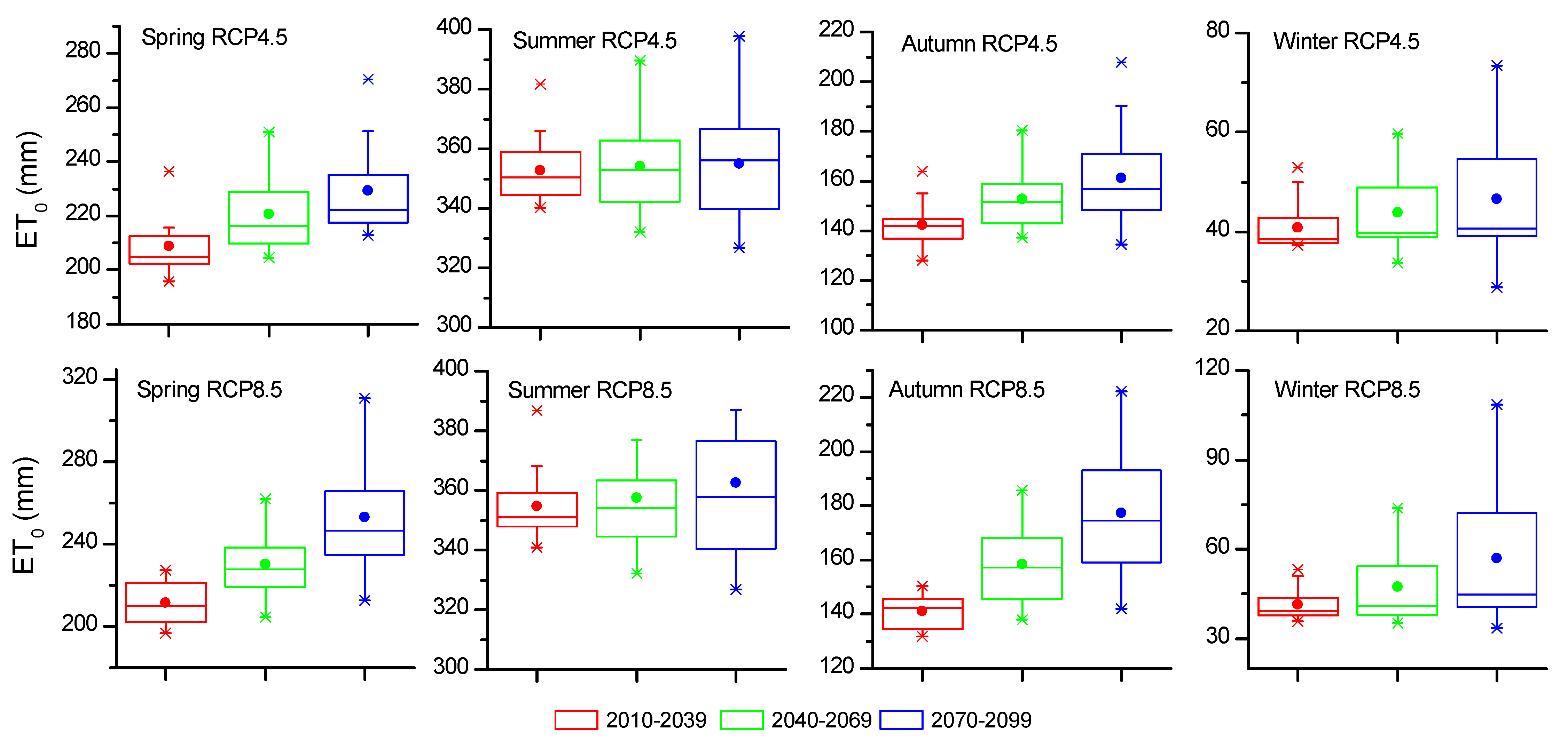
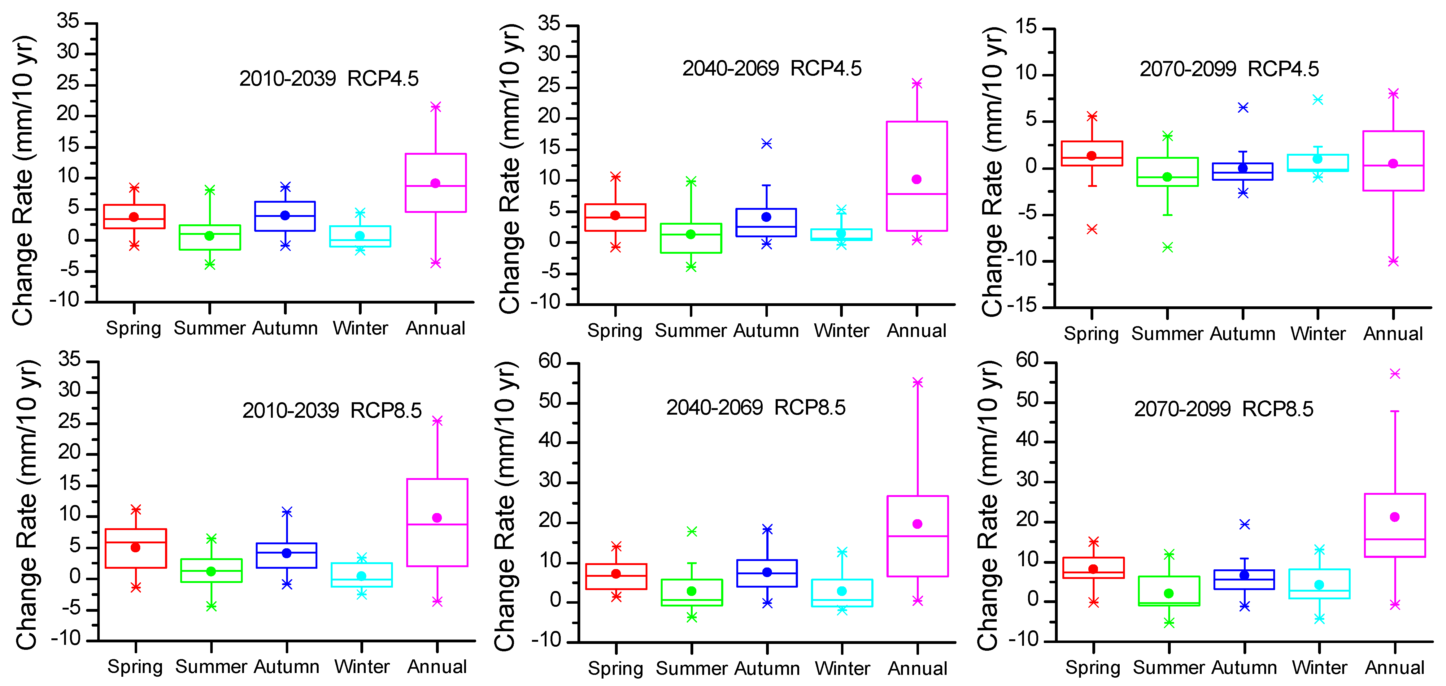
3.2.2. Decadal and Seasonal Future ET₀ Projections

Furthermore, we divided the projection horizons into three sub-periods: first, a sub-period (from 2010 to 2039) named as the near term; a second sub-period (from 2040 to 2069) as the mid term; and a third (2070 to 2099) as the long term. The statistics of ET₀ for the three periods have been illustrated in Figure 8. It is evident that the magnitudes and variations appear to increase with an increase in time at the two warming scenarios, and it is becoming more obvious with increasing uncertainty under the RCP8.5. For the near term, the ET₀ values varied between 725–755 mm under the RCP4.5 warming scenario and between 720–765 mm under the RCP8.5 warming scenario. The ranges of ET₀ in the mid term are found to be approximately 740–805 mm and 750–830 mm for the RCP4.5 and RCP8.5 scenarios, respectively; and in the long term they are found to be approximately 745–840 mm and 770–890 mm for the RCP4.5 and RCP8.5 scenarios, respectively.

Figure 9 shows the simulated the ET₀ for the four seasons. The magnitudes and variations in ET₀ for the three periods in the four seasons are seen to agree with the annual properties for both warming scenarios. That is, the summer ET₀ is found to be the largest compared to the other three seasons, with median values of approximately 350 mm, 353 mm and 357 mm for RCP4.5 and approximately 351 mm, 355 mm and 357 mm for RCP8.5 from the near to long term, respectively. The winter ET₀ value is found to be the lowest, with median values of approximately 38 mm, 40 mm and 41 mm for RCP4.5 and approximately 40 mm, 42 mm and 44 mm for RCP8.5 from the near to long term, respectively. It should be noted that the median of the summer and winter changes in ET₀ from the near to long term is lower when compared to spring and autumn. This implies that future ET₀ variations are likely to occur mainly in the spring and autumn seasons.

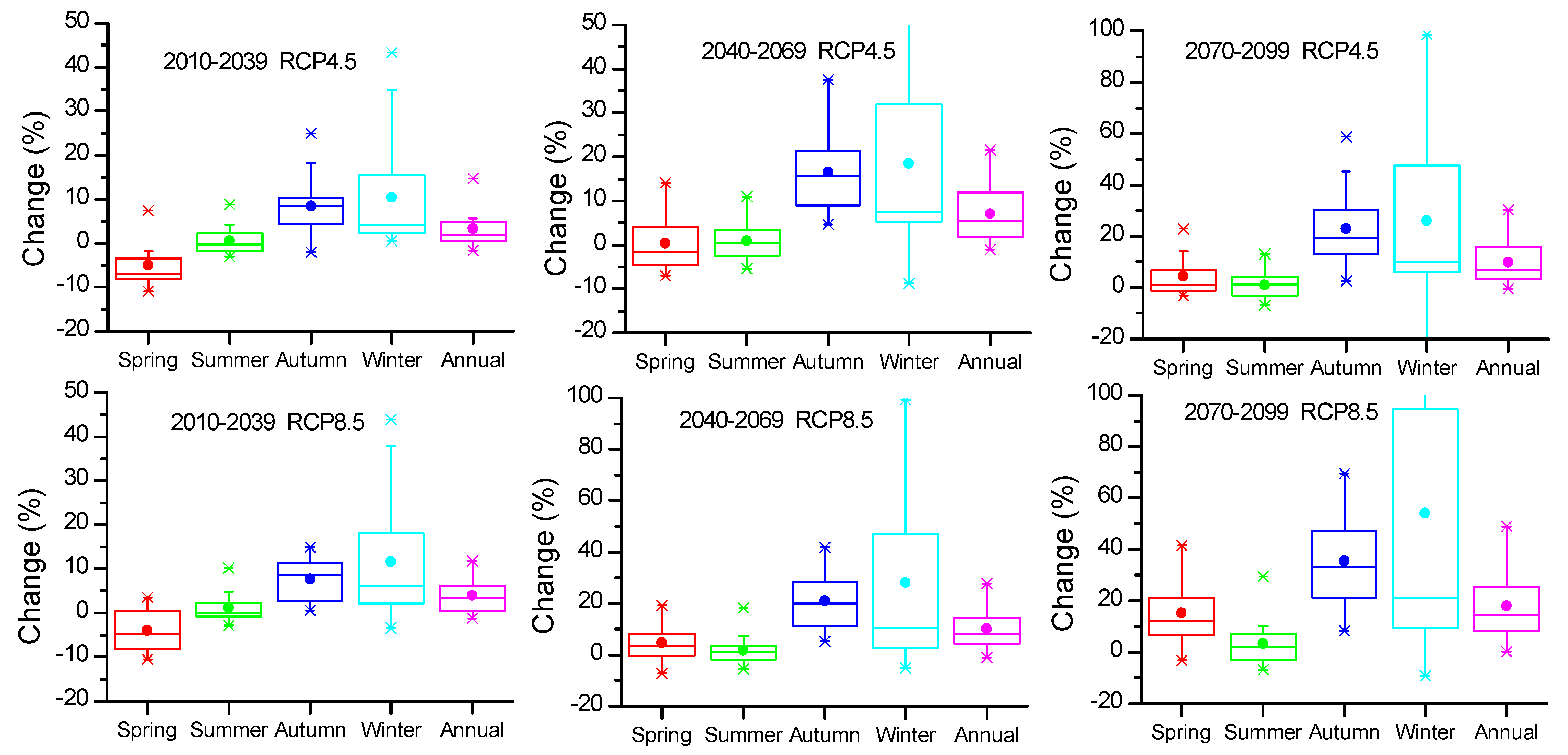
3.3. Projection of Future ET₀ Variation

In order to simulate the tendency of future ET₀ variation, the Sen Slope method was applied [78]. Figure 10 shows the seasonal and annual ET₀ change rate for the three periods considered under the two RCP warming scenarios. Seasonally, the ET₀ change rate for the summer and the winter seasons appear to be nearly close to 0 during the three periods. However, we can apparently deduce that the increasing trend is likely to occur in the spring and autumn seasons. This is more obvious under the RCP8.5 compared to the RCP4.5 warming scenarios. Annually, the ET₀ data is likely to exhibit an increase, with a median rate of 7.5 mm/decade during the near term and mid term, and nearly close to 0 during the long term under the RCP4.5 warming scenarios. Moreover, for the RCP8.5 scenario, the median rate of ET₀ for the near term is found to be approximately 8.2 mm/decade, and for the mid term is approximately 15 mm/decade.

Figure 11 shows the relative changes in simulated ET₀ compared to the historical period (1961–2005). Evidently, the results show that the spring season ET₀ is likely to decrease by approximately 5% and 10% for the RCP4.5 and RCP8.5 warning scenarios, respectively, in the near term when compared with the period 1961–2005. However, the summer ET₀ values are likely to be almost consistent with the median value, being close to 0. The relative change in the autumn seasonal ET₀ is shown to be largest when compared to the other three seasons, with a highest median value for both warming scenarios and three considered periods. The winter ET₀, however, is likely to increase with a large degree of uncertainty. It is also possible that the uncertainty is likely to increase over the passage of time. For the annual changes in ET₀, the present results show that the relative changes are likely to be approximately 2%, 5% and 6% during the near-, mid- and long-term periods, respectively, under the RCP4.5 warming scenario; whereas it is likely to be approximately 2%, 7% and 13% during the three periods considered, respectively, under the RCP8.5 warming scenario.

4. Discussion and Summary

In reality, the true reference evapotranspiration (ET₀) can be obtained experimentally; however, in many situations there are difficulties carrying out measurements. As a result, the FAO-56 Penman–Monteith formulation for ET₀ is often accepted. This paper aimed to downscale monthly ET₀ using two less-explored learning algorithms based on ELM and SVR approaches by developing and validating the regression relationships between station-based ET₀ and large-scale atmospheric variables from a suite of eight relatively high spatial-resolution GCM outputs. Without considering the physical relationship between ET₀ and the climatic variables, the approaches presented in this paper were able to successfully downscale local ET₀ time series by building on the appropriate statistical relationships between the observed ET₀ (FAO-56 PM ET₀) with the surface–atmospheric features, whereby an ensemble of models was studied in terms of the large-scale and transient changes of the host GCM models. In this regard, the downscaling approaches applied in the present study, where a study of future trends in ET₀ is based on many GCM selections, simulation methods and warming scenarios and trajectories, are considered as invaluable tools for advancing the relevance of hydrological models for more meaningful local-scale applications.

This study has projected the future variability of ET₀ by applying the ELM and SVR approaches in a mountainous inland watershed of north-west China. A total of eight relatively high spatial-resolution GCM-based model outputs from CMIP5 simulations were employed to downscale for the historical period (1960–2005) and the future period (2010–2099) ET₀ under the RCP4.5 and RCP8.5 warming scenarios.

The AI-based ELM and SVR approaches revealed satisfactory performances in estimating the ET₀ data. Moreover, the performance of the SVR model for ET₀ projection is modestly better than the ELM model. The future variation in ET₀ appeared to occur mainly in the spring and autumn seasons, while in the summer and winter seasons, the ET₀ changes were very small. Annually, the rate of increase in ET₀ was found to be approximately 7.5 mm/decade for the near and middle terms, and nearly close to 0 for the long-term period under the RCP4.5 warming scenario. By contrast, for RCP8.5, the rate of increase in ET₀ for the near term was found to be approximately 8.2 mm/decade, and 15 mm/decade for the mid-term and long-term periods. Compared to the historical period in this study (1960–2005), the relative changes were found to be approximately 2%, 5% and 6% in the near-, mid- and long-term periods, respectively, under the RCP4.5 warming scenario, whereas they were approximately 2%, 7% and 13% for the three periods, respectively, under the RCP8.5 warming scenario.

Compared to the uncertainties from the different estimation formulations and different inputs from atmospheric variables, the uncertainties derived from the different GCM outputs are a prime source of a model’s fidelity [81]. Thus, it is necessary to employ multiple GCM outputs to be used as predictor variables when a local-scale climatic property needs to be projected.

The AI-based methods developed in this case study appear to promise soft-computing approaches for the future variability of reference evapotranspiration. However, there were some unavoidable uncertainties; for example, we tested 8 GCM-based model outputs which might not completely represent future climate change. More GCM-based model outputs should be adopted. Moreover, future work should test more AI-based methods for investigating ET₀ projection.

References

1. Antonopoulos, V.Z.; Antonopoulos, A.V. Daily reference evapotranspiration estimates by artificial neural networks technique and empirical equations using limited input climate variables. Comput. Electron. Agric. 2017, 132, 86–96. [Google Scholar] [CrossRef]
2. Fan, J.; Wu, L.; Zhang, F.; Xiang, Y.; Zheng, J. Climate change effects on reference crop evapotranspiration across different climatic zones of china during 1956–2015. J. Hydrol. 2016, 542, 923–937. [Google Scholar] [CrossRef]
3. Wang, W.; Xing, W.; Shao, Q. How large are uncertainties in future projection of reference evapotranspiration through different approaches? J. Hydrol. 2015, 524, 696–700. [Google Scholar] [CrossRef]
4. Feng, Y.; Peng, Y.; Cui, N.; Gong, D.; Zhang, K. Modeling reference evapotranspiration using extreme learning machine and generalized regression neural network only with temperature data. Comput. Electron. Agric. 2017, 136, 71–78. [Google Scholar] [CrossRef]
5. Abdullah, S.S.; Malek, M.A.; Abdullah, N.S.; Kisi, O.; Yap, K.S. Extreme learning machines: A new approach for prediction of reference evapotranspiration. J. Hydrol. 2015, 527, 184–195. [Google Scholar] [CrossRef]
6. Shiri, J.; Kişi, Ö.; Landeras, G.; López, J.J.; Nazemi, A.H.; Stuyt, L.C.P.M. Daily reference evapotranspiration modeling by using genetic programming approach in the basque country (northern spain). J. Hydrol. 2012, 414–415, 302–316. [Google Scholar] [CrossRef]
7. Li, Y.; Yao, N.; Chau, H.W. Influences of removing linear and nonlinear trends from climatic variables on temporal variations of annual reference crop evapotranspiration in xinjiang, china. Sci. Total Environ. 2017, 592, 680–692. [Google Scholar] [CrossRef] [PubMed]
8. Gao, Z.; He, J.; Dong, K.; Li, X. Trends in reference evapotranspiration and their causative factors in the west liao river basin, china. Agric. For. Meteorol. 2017, 232, 106–117. [Google Scholar] [CrossRef]
9. Lu, J.; Sun, G.; Mcnulty, S.G.; Amatya, D.M. A comparison of six potential evapotranspiration methods for regional use in the southeastern united states. J. Am. Water Resour. Assoc. 2005, 41, 621–633. [Google Scholar] [CrossRef]
10. Goyal, R.K. Sensitivity of evapotranspiration to global warming: A case study of arid zone of rajasthan (india). Agr. Water Manag. 2004, 69, 1–11. [Google Scholar] [CrossRef]
11. Temesgen, B.; Eching, S.; Davidoff, B.; Frame, K. Comparison of some reference evapotranspiration equations for california. J. Irrig. Drain. Eng. 2005, 131, 73–84. [Google Scholar] [CrossRef]
12. Liu, X.; Xu, C.; Zhong, X.; Li, Y.; Yuan, X.; Cao, J. Comparison of 16 models for reference crop evapotranspiration against weighing lysimeter measurement. Agric. Water Manag. 2017, 184, 145–155. [Google Scholar] [CrossRef]
13. Xing, W.; Wang, W.; Shao, Q.; Peng, S.; Yu, Z.; Yong, B.; Taylor, J. Changes of reference evapotranspiration in the haihe river basin: Present observations and future projection from climatic variables through multi-model ensemble. Glob. Planet. Chang. 2014, 115, 1–15. [Google Scholar] [CrossRef]
14. Kisi, O.; Sanikhani, H.; Zounemat-Kermani, M.; Niazi, F. Long-term monthly evapotranspiration modeling by several data-driven methods without climatic data. Comput. Electron. Agric. 2015, 115, 66–77. [Google Scholar] [CrossRef]
15. Wang, Z.; Xie, P.; Lai, C.; Chen, X.; Wu, X.; Zeng, Z.; Li, J. Spatiotemporal variability of reference evapotranspiration and contributing climatic factors in china during 1961–2013. J. Hydrol. 2017, 544, 97–108. [Google Scholar] [CrossRef]
16. Chau, K.W.; Wu, C.L. A hybrid model coupled with singular spectrum analysis for daily rainfall prediction. J. Hydroinf. 2010, 12, 458. [Google Scholar] [CrossRef]
17. Wu, C.L.; Chau, K.W.; Fan, C. Prediction of rainfall time series using modular artificial neural networks coupled with data-preprocessing techniques. J. Hydrol. 2010, 389, 146–167. [Google Scholar] [CrossRef]
18. Chen, X.Y.; Chau, K.W.; Busari, A.O. A comparative study of population-based optimization algorithms for downstream river flow forecasting by a hybrid neural network model. Eng. Appl. Artif. Intell. 2015, 46, 258–268. [Google Scholar] [CrossRef]
19. Gholami, V.; Chau, K.W.; Fadaee, F.; Torkaman, J.; Ghaffari, A. Modeling of groundwater level fluctuations using dendrochronology in alluvial aquifers. J. Hydrol. 2015, 529, 1060–1069. [Google Scholar] [CrossRef]
20. Taormina, R.; Chau, K.-W. Data-driven input variable selection for rainfall–runoff modeling using binary-coded particle swarm optimization and extreme learning machines. J. Hydrol. 2015, 529, 1617–1632. [Google Scholar] [CrossRef]
21. Wang, W.-c.; Chau, K.-w.; Xu, D.-m.; Chen, X.-Y. Improving forecasting accuracy of annual runoff time series using arima based on eemd decomposition. Water Resour. Manag. 2015, 29, 2655–2675. [Google Scholar] [CrossRef]
22. Kumar, M.; Raghuwanshi, N.S.; Singh, R.; Wallender, W.W.; Pruitt, W.O. Estimating evapotranspiration using artificial neural network. J. Irrig. Drain. Eng. 2002, 128, 224–233. [Google Scholar] [CrossRef]
23. Kisi, O. The potential of different ann techniques in evapotranspiration modelling. Hydrol. Process. 2008, 22, 2449–2460. [Google Scholar] [CrossRef]
24. Kisi, O.; Cengiz, T.M. Fuzzy genetic approach for estimating reference evapotranspiration of turkey: Mediterranean region. Water Resour. Manag. 2013, 27, 3541–3553. [Google Scholar] [CrossRef]
25. Kim, S.; Kim, H.S. Neural networks and genetic algorithm approach for nonlinear evaporation and evapotranspiration modeling. J. Hydrol. 2008, 351, 299–317. [Google Scholar] [CrossRef]
26. Shiri, J.; Dierickx, W.; Pour-Ali Baba, A.; Neamati, S.; Ghorbani, M.A. Estimating daily pan evaporation from climatic data of the state of illinois, USA using adaptive neuro-fuzzy inference system (anfis) and artificial neural network (ann). Hydrol. Res. 2011, 42, 491. [Google Scholar] [CrossRef]
27. Shiri, J.; Nazemi, A.H.; Sadraddini, A.A.; Landeras, G.; Kisi, O.; Fakheri Fard, A.; Marti, P. Comparison of heuristic and empirical approaches for estimating reference evapotranspiration from limited inputs in iran. Comput. Electron. Agric. 2014, 108, 230–241. [Google Scholar] [CrossRef]
28. Kisi, O.; Cimen, M. Evapotranspiration modelling using support vector machines. Hydrol. Sci. J. 2009, 54, 918–928. [Google Scholar] [CrossRef]
29. Kisi, O. Modeling reference evapotranspiration using three different heuristic regression approaches. Agric. Water Manag. 2016, 169, 162–172. [Google Scholar] [CrossRef]
30. Rahimikhoob, A.; Asadi, M.; Mashal, M. A comparison between conventional and m5 model tree methods for converting pan evaporation to reference evapotranspiration for semi-arid region. Water Resour. Manag. 2013, 27, 4815–4826. [Google Scholar] [CrossRef]
31. Feng, Y.; Cui, N.; Zhao, L.; Hu, X.; Gong, D. Comparison of elm, gann, wnn and empirical models for estimating reference evapotranspiration in humid region of southwest china. J. Hydrol. 2016, 536, 376–383. [Google Scholar] [CrossRef]
32. Deo, R.C.; Şahin, M. Application of the artificial neural network model for prediction of monthly standardized precipitation and evapotranspiration index using hydrometeorological parameters and climate indices in eastern australia. Atmos. Res. 2015, 161, 65–81. [Google Scholar] [CrossRef]
33. Patil, A.P.; Deka, P.C. An extreme learning machine approach for modeling evapotranspiration using extrinsic inputs. Comput. Electron. Agric. 2016, 121, 385–392. [Google Scholar] [CrossRef]
34. Wen, X.; Si, J.; He, Z.; Wu, J.; Shao, H.; Yu, H. Support-vector-machine-based models for modeling daily reference evapotranspiration with limited climatic data in extreme arid regions. Water Resour. Manag. 2015, 29, 3195–3209. [Google Scholar] [CrossRef]
35. Tabari, H.; Kisi, O.; Ezani, A.; Hosseinzadeh Talaee, P. Svm, anfis, regression and climate based models for reference evapotranspiration modeling using limited climatic data in a semi-arid highland environment. J. Hydrol. 2012, 444–445, 78–89. [Google Scholar] [CrossRef]
36. Yin, Z.; Wen, X.; Feng, Q.; He, Z.; Zou, S.; Yang, L. Integrating genetic algorithm and support vector machine for modeling daily reference evapotranspiration in a semi-arid mountain area. Hydrol. Res. 2017, 48, 1177–1191. [Google Scholar] [CrossRef]
37. Kisi, O. Least squares support vector machine for modeling daily reference evapotranspiration. Irrig. Sci. 2013, 31, 611–619. [Google Scholar] [CrossRef]
38. Huang, G.-B.; Zhu, Q.-Y.; Siew, C.-K. Extreme learning machine: A new learning scheme of feedforward neural networks. In Proceedings of the 2004 IEEE International Joint Conference on Neural Networks (IEEE Cat. No.04CH37541), Budapest, Hungary, 25–29 July 2004. [Google Scholar]
39. Wang, X.; Han, M. Online sequential extreme learning machine with kernels for nonstationary time series prediction. Neurocomputing 2014, 145, 90–97. [Google Scholar] [CrossRef]
40. Cambria, E.; Huang, G.B.; Kasun, L.L.C.; Zhou, H.; Vong, C.M.; Lin, J.; Yin, J.; Cai, Z.; Liu, Q.; Li, K.; et al. Extreme learning machines [trends & controversies]. IEEE Intell. Syst. 2013, 28, 30–59. [Google Scholar]
41. Deo, R.C.; Downs, N.; Parisi, A.; Adamowski, J.; Quilty, J. Very short-term reactive forecasting of the solar ultraviolet index using an extreme learning machine integrated with the solar zenith angle. Environ. Res. 2017, 155, 141–166. [Google Scholar] [CrossRef] [PubMed]
42. Deo, R.C.; Şahin, M. Application of the extreme learning machine algorithm for the prediction of monthly effective drought index in eastern australia. Atmos. Res. 2015, 153, 512–525. [Google Scholar] [CrossRef]
43. Deo, R.C.; Sahin, M. An extreme learning machine model for the simulation of monthly mean streamflow water level in eastern queensland. Environ. Monit. Assess. 2016, 188, 90. [Google Scholar] [CrossRef] [PubMed]
44. Deo, R.C.; Samui, P.; Kim, D. Estimation of monthly evaporative loss using relevance vector machine, extreme learning machine and multivariate adaptive regression spline models. Stoch. Environ. Res. Risk Assess. 2015, 1–16. [Google Scholar] [CrossRef]
45. Deo, R.C.; Syktus, J.; McAlpine, C.; Lawrence, P.; McGowan, H.; Phinn, S.R. Impact of historical land cover change on daily indices of climate extremes including droughts in eastern australia. Geophys. Res. Lett. 2009, 36. [Google Scholar] [CrossRef]
46. Deo, R.C.; Tiwari, M.K.; Adamowski, J.F.; Quilty, M.J. Forecasting effective drought index using a wavelet extreme learning machine (w-elm) model. Stoch. Environ. Res. Risk Assess. 2016, 1–30. [Google Scholar] [CrossRef]
47. Yaseen, Z.M.; Jaafar, O.; Deo, R.C.; Kisi, O.; Adamowski, J.; Quilty, J.; El-Shafie, A. Stream-flow forecasting using extreme learning machines: A case study in a semi-arid region in iraq. J. Hydrol. 2016. [Google Scholar] [CrossRef]
48. Huang, G.; Huang, G.B.; Song, S.; You, K. Trends in extreme learning machines: A review. Neural Netw. 2015, 61, 32–48. [Google Scholar] [CrossRef] [PubMed]
49. Gocic, M.; Petković, D.; Shamshirband, S.; Kamsin, A. Comparative analysis of reference evapotranspiration equations modelling by extreme learning machine. Comput. Electron. Agric. 2016, 127, 56–63. [Google Scholar] [CrossRef]
50. Pachauri, R.K.; Allen, M.R.; Barros, V.R.; Broome, J.; Cramer, W.; Christ, R.; Chruch, J.A.; Clarke, L.; Dahe, Q.; Dasgupta, P. Climate Change 2014: Synthesis Report; Contribution of Working Groups I, II and III to the Fifth Assessment Report of the Intergovernmental Panel on Climate Change; IPCC: Geneva, Switzerland, 2014. [Google Scholar]
51. Piao, S.; Ciais, P.; Huang, Y.; Shen, Z.; Peng, S.; Li, J.; Zhou, L.; Liu, H.; Ma, Y.; Ding, Y.; et al. The impacts of climate change on water resources and agriculture in china. Nature 2010, 467, 43–51. [Google Scholar] [CrossRef] [PubMed]
52. Irmak, S.; Kabenge, I.; Skaggs, K.E.; Mutiibwa, D. Trend and magnitude of changes in climate variables and reference evapotranspiration over 116-yr period in the platte river basin, central nebraska–USA. J. Hydrol. 2012, 420–421, 228–244. [Google Scholar] [CrossRef]
53. Tabari, H.; Aghajanloo, M.-B. Temporal pattern of aridity index in iran with considering precipitation and evapotranspiration trends. Int. J. Climatol. 2013, 33, 396–409. [Google Scholar] [CrossRef]
54. Palumbo, A.D.; Vitale, D.; Campi, P.; Mastrorilli, M. Time trend in reference evapotranspiration: Analysis of a long series of agrometeorological measurements in southern italy. Irrig. Drain. Syst. 2011, 25, 395–411. [Google Scholar] [CrossRef]
55. Piticar, A.; Mihăilă, D.; Lazurca, L.G.; Bistricean, P.-I.; Puţuntică, A.; Briciu, A.-E. Spatiotemporal distribution of reference evapotranspiration in the republic of moldova. Theor. Appl. Climatol. 2016, 124, 1133–1144. [Google Scholar] [CrossRef]
56. Bandyopadhyay, A.; Bhadra, A.; Raghuwanshi, N.S.; Singh, R. Temporal trends in estimates of reference evapotranspiration over india. J. Hydrol. Eng. 2009, 14, 508–515. [Google Scholar] [CrossRef]
57. Li, Z.; Zheng, F.-L.; Liu, W.-Z. Spatiotemporal characteristics of reference evapotranspiration during 1961–2009 and its projected changes during 2011–2099 on the loess plateau of china. Agric. For. Meteorol. 2012, 154–155, 147–155. [Google Scholar] [CrossRef]
58. Gao, X.; Zhao, Q.; Zhao, X.; Wu, P.; Pan, W.; Gao, X.; Sun, M. Temporal and spatial evolution of the standardized precipitation evapotranspiration index (spei) in the loess plateau under climate change from 2001 to 2050. Sci. Total Environ. 2017, 595, 191–200. [Google Scholar] [CrossRef] [PubMed]
59. Peng, S.; Ding, Y.; Wen, Z.; Chen, Y.; Cao, Y.; Ren, J. Spatiotemporal change and trend analysis of potential evapotranspiration over the loess plateau of china during 2011–2100. Agric. For. Meteorol. 2017, 233, 183–194. [Google Scholar] [CrossRef]
60. Kundu, S.; Khare, D.; Mondal, A. Future changes in rainfall, temperature and reference evapotranspiration in the central india by least square support vector machine. Geosci. Front. 2017, 8, 583–596. [Google Scholar] [CrossRef]
61. Aksornsingchai, P.; Srinilta, C. Statistical downscaling for rainfall and temperature prediction in thailand. In Proceedings of the international multiconference of engineers and computer scientists, Hong Kong, China, 16–18 March 2011. [Google Scholar]
62. Tripathi, S.; Srinivas, V.; Nanjundiah, R.S. Downscaling of precipitation for climate change scenarios: A support vector machine approach. J. Hydrol. 2006, 330, 621–640. [Google Scholar] [CrossRef]
63. Sachindra, D.; Huang, F.; Barton, A.; Perera, B. Least square support vector and multi-linear regression for statistically downscaling general circulation model outputs to catchment streamflows. Int. J. Climatol. 2013, 33, 1087–1106. [Google Scholar] [CrossRef]
64. Kharin, V.; Scinocca, J. The impact of model fidelity on seasonal predictive skill. Geophys. Res. Lett. 2012, 39. [Google Scholar] [CrossRef]
65. Yin, Z.; Feng, Q.; Zou, S.; Yang, L. Assessing variation in water balance components in mountainous inland river basin experiencing climate change. Water 2016, 8, 472. [Google Scholar] [CrossRef]
66. Cheng, G.; Li, X.; Zhao, W.; Xu, Z.; Feng, Q.; Xiao, S.; Xiao, H. Integrated study of the water–ecosystem–economy in the heihe river basin. Natl. Sci. Rev. 2014, 1, 413–428. [Google Scholar] [CrossRef]
67. Marsland, S.; Bi, D.; Uotila, P.; Fiedler, R.; Griffies, S.; Lorbacher, K.; O'Farrell, S.; Sullivan, A.; Uhe, P.; Zhou, X.; et al. Evaluation of access climate model ocean diagnostics in cmip5 simulations. Aust. Meteorol. Oceanogr. J. 2013, 63, 101–119. [Google Scholar] [CrossRef]
68. Ren, H.-L.; Wu, J.; Zhao, C.-B.; Cheng, Y.-J.; Liu, X.-W. Mjo ensemble prediction in bcc-csm1.1(m) using different initialization schemes. Atmos. Ocean. Sci. Lett. 2016, 9, 60–65. [Google Scholar] [CrossRef]
69. Voldoire, A.; Sanchez-Gomez, E.; Salas y Mélia, D.; Decharme, B.; Cassou, C.; Sénési, S.; Valcke, S.; Beau, I.; Alias, A.; Chevallier, M.; et al. The cnrm-cm5.1 global climate model: Description and basic evaluation. Clim. Dyn. 2013, 40, 2091–2121. [Google Scholar] [CrossRef] [Green Version]
70. Martin, G.M.; Bellouin, N.; Collins, W.J.; Culverwell, I.D.; Halloran, P.R.; Hardiman, S.C.; Hinton, T.J.; Jones, C.D.; McDonald, R.E.; McLaren, A.J.; et al. The hadgem2 family of met office unified model climate configurations. Geosci. Model Dev. 2011, 4, 723–757. [Google Scholar]
71. Watanabe, M.; Suzuki, T.; O’ishi, R.; Komuro, Y.; Watanabe, S.; Emori, S.; Takemura, T.; Chikira, M.; Ogura, T.; Sekiguchi, M.; et al. Improved climate simulation by miroc5: Mean states, variability, and climate sensitivity. J. Clim. 2010, 23, 6312–6335. [Google Scholar] [CrossRef]
72. Yukimoto, S.; Adachi, Y.; Hosaka, M.; Sakami, T.; Yoshimura, H.; Hirabara, M.; Tanaka, T.Y.; Shindo, E.; Tsujino, H.; Deushi, M.; et al. A new global climate model of the meteorological research institute: Mri-cgcm3 —model description and basic performance&mdash. J. Meteorol. Soc. Jpn. Ser. II 2012, 90A, 23–64. [Google Scholar]
73. Allen, R.G.; Pereira, L.S.; Raes, D.; Smith, M. Crop Evapotranspiration: Guidelines for Computing Crop Requirements Fao Irrigation and Drainage Paper No. 56; FAO: Rome, Italy, 1998. [Google Scholar]
74. Huang, G.-B.; Zhu, Q.-Y.; Siew, C.-K. Extreme learning machine: Theory and applications. Neurocomputing 2006, 70, 489–501. [Google Scholar] [CrossRef]
75. Deo, R.C.; Şahin, M. An extreme learning machine model for the simulation of monthly mean streamflow water level in eastern queensland. Environ. Monit. Assess. 2016. [Google Scholar] [CrossRef]
76. Vapnik, V. The Nature of Statistical Learning Theory; Springer: New York, NY, USA, 1995. [Google Scholar]
77. Tezel, G.; Buyukyildiz, M. Monthly evaporation forecasting using artificial neural networks and support vector machines. Theor. Appl. Climatol. 2016, 124, 69–80. [Google Scholar] [CrossRef]
78. Yang, L.; Feng, Q.; Li, C.; Si, J.; Wen, X.; Yin, Z. Detecting climate variability impacts on reference and actual evapotranspiration in the taohe river basin, nw china. Hydrol. Res. 2017, 48, 596–612. [Google Scholar] [CrossRef]
79. Chai, T.; Draxler, R.R. Root mean square error (rmse) or mean absolute error (mae)?–arguments against avoiding rmse in the literature. Geosci. Model Dev. 2014, 7, 1247–1250. [Google Scholar] [CrossRef]
80. Nash, J.; Sutcliffe, J. River flow forecasting through conceptual models part i—A discussion of principles. J. Hydrol. 1970, 10, 282–290. [Google Scholar] [CrossRef]
81. Thompson, J.R.; Green, A.J.; Kingston, D.G. Potential evapotranspiration-related uncertainty in climate change impacts on river flow: An assessment for the mekong river basin. J. Hydrol. 2014, 510, 259–279. [Google Scholar] [CrossRef]
Figure 1. (a) and (b) Location of the Yingluoxia (YLX) Watershed; (c) mean monthly rainfall and temperature at the Yeniugou weather station from 1961 to 2013; (d) the global climate model (GCM) points and grids of ACCESS1.0, ACCESS1.3, HadGEM2-CC and HadGEM2-ES; (e) the GCM points and grids of BCC-CSM1.1(m) and MRI-CGCM3; (f) the GCM points and grids of CNRM-CM5 and MIROC5.
Water 09 00880 g001
Figure 2. Schematic diagram for the modelling process followed to generate future reference evapotranspiration (ET0) projections.
Water 09 00880 g002
Figure 3. Scatter plots for the historical ET0 (1961–2005) calculated by the Penman–Monteith equation with the observed meteorological data downscaled by the extreme-learning machine (ELM) and support vector regression (SVR) approaches derived for the eight GCM outputs.
Water 09 00880 g003
Figure 4. Performances for the ELM and SVR models applied to the eight GCM outputs for downscaling the ET0 in validation period (1990–2005).
Water 09 00880 g004
Figure 5. Boxplots for the performances of ELM (top) and SVR (bottom) models for ET0, calculated for different periods.
Water 09 00880 g005
Figure 6. Performances of the ELM and SVR model for downscaling GCM-derived ET0 at seasonal scales during the 1961–2005 period.
Water 09 00880 g006
Figure 7. Results of future ET0 projection derived from GCM outputs under the RCP4.5 and RCP8.5 scenarios.
Water 09 00880 g007
Figure 8. Boxplots for the future annual ET0 projection under the RCP4.5 and RCP8.5 scenarios.
Water 09 00880 g008
Figure 9. Boxplots for the future seasonal ET0 projection under the RCP4.5 and RCP8.5 scenarios.
Water 09 00880 g009
Figure 10. Boxplots for the change slope of future ET0 at seasonal and annual scales calculated by the Sen Slope method.
Water 09 00880 g010
Figure 11. Boxplots for percentage change of future ET0 related to the period 1961–2005 at seasonal and annual scales.
Water 09 00880 g011