“In-Process Type” Dynamic Muskingum Model Parameter Estimation Method
by
 , ,
, ,
Gang Zhang
1,* ,
,
Tuo Xie
1,
Lei Zhang
1,
Xia Hua
2,
Chen Wu
1,
Xi Chen
1,
Fangfeng Li
1 and
Bin Zhao
1 1
Institute of Water Resources and Hydro-Electric Engineering, Xi’an University of Technology, Xi’an 710048, China
2
State Grid Gansu Electric Power Company, Gansu Electric Power Research Institute, Lanzhou 730050, China
*
Author to whom correspondence should be addressed.
Water 2017, 9(11), 849; https://doi.org/10.3390/w9110849
Submission received: 29 August 2017
/
Revised: 30 October 2017
/
Accepted: 31 October 2017
/
Published: 2 November 2017
Abstract
:This paper discusses the Muskingum model as a novel parameter estimation method. Sixty representative floods over the past four decades serve as research objects; a linear Muskingum model and Pigeon-inspired optimization (PIO) algorithm are used to obtain the parameters of each flood. The proposed “in-process type” dynamic parameter estimation (IP-DPE) method is used to establish the characteristic attributes set of 50 floods. The characteristic attributes set refers to a set of parameters that could describe the shape, magnitude, and duration of the flood before flood peak; they are the input, whereas parameters K and x of each flood are the output to establish a Neural Network model. Then we input flood characteristic attributes to obtain flood parameters when estimating flood parameters practically. Ten floods were used to test the parameter estimation and flood routing efficacy. The results show that the IP-DPE method can quickly identify parameters and facilitate accurate river flood forecasting.
1. Introduction
The Muskingum model has been commonly utilized for river flood forecasting across various parts of the world since it was first proposed in the 1930s [1,2]. For the model to work properly, its parameters must be accurately estimated. Several methods for such parameter estimation have been proposed in recent years, including trial-and-error [3], the least-square method [4,5,6], and nonlinear programming [7,8]. In practice, however, these approaches come with high computational complexity, poor universality, and susceptibility to local optima [9]. Advancements in computer technology have allowed for innovative parameter estimation optimization algorithms such as the Genetic Algorithm [10,11], Particle Swarm Optimization Algorithm [12,13], Chaotic Particle Swarm Optimization Algorithm [14], and Ant Colony Algorithm [15].
Both traditional approaches and optimized algorithms have assisted in developing a useful Muskingum model parameter estimation method [2]. However, there still are important problems to be resolved:
- (1)
- At present, most methods are developed with the sole focus on improving the simulation accuracy of one flood [16,17,18], such as in [16], where the average relative errors obtained from four algorithms were 1.16%, 1.11%, 1.13%, and 1.10%, respectively, and the improvement was inherently limited. Also, although the obtained flood parameters could forecast the selected flood, they did not validate whether the parameters can be applied to the other floods, and the practicality of the model is generally ignored.
- (2)
Although the floods occur in the same river channel, their model parameters may not be the same and sometimes have big differences [9,20]. The ultimate goal of flood forecasting, to this effect, is to secure parameters that are ultimately applicable to the entire river channel. Ye et al. [21] used the mean value of estimated parameters as final parameter values. Wang et al. [19] established parameters according to flow classifications (i.e., flood magnitudes), and this technique was also used in another study [22]. Both methods have relatively high forecasting accuracy but still come with limited performance. To remedy these problems, we suggest that:
- (1)
- The Muskingum model parameters should not be unique to a given river course, and should change dynamically with the characteristics of different floods (e.g., flood flow, velocity, flood volume).
- (2)
- The Muskingum model parameters should not be determined by one flood or the mean of several floods, it should be obtained from the real-time dynamic parameter estimation.
This paper proposes the “in-process type” dynamic parameter estimation Muskingum model based on the Back-Propagation Artificial Neural Network (BP-ANN). We selected several floods with different magnitudes over the past 40 years from a river channel (between Sunkou and Gaocun Hydrometric Stations) of the Yellow River and applied the Pigeon-inspired optimization (PIO) algorithm to estimate their respective parameters. We compared the results against three other methods to validate the applicability of the PIO algorithm, then extracted the characteristic attributes of each flood—which showed the form feature, different orders of magnitude, and duration of the flood—and analyzed the correlation between each attribute and parameter. The characteristic attributes were input to the BP-Neural Network, and the resulting optimization algorithm estimates were taken as output to train the Neural Network model. Finally, the trained model was applied to several floods to validate the reliability and practicality of the proposed method.
2. Materials and Methods
2.1. Muskingum Model
2.1.1. Introduction to Muskingum Model Theories
The flood routing of a river course is meant to deduce the flood process of the downstream section according to the process of the upstream section. The Muskingum model is an effective channel flood routing model that has been widely used. This method is mainly used to carry out flood routing of a river course by establishing a river channel storage equation and solving the water balance equation simultaneously. The basic equation for flood routing in the Muskingum model is:
in which W is the river course storage volume, t is the time, I and Q are the inflow and outflow of the river reach, respectively, x is the weighting factor, and K is a constant of the Muskingum model for the river reach.
The differential Equation (1) can be discretized as follows:
where and are the calculated outflow and the observed outflow, respectively, at the calculation time i, is the inflow at the calculation time i, n is the total amount of time, , and are flow routing coefficients, and satisfy the following:
The flood flow routing equation of the Muskingum model consists of Equations (2) and (3). As discussed above, parameter estimation is one of the most important aspects of correctly applying the Muskingum model. It involves the estimation of parameters K and x (or parameters ).
2.1.2. Establishing the Muskingum Parameter Optimization Model
According to Equations (2) and (3), the parameter optimization problem of the Muskingum model can be transformed as follows:
In the Equation (5), the objective function refers to minimizing the relative error sum between calculated outflow and observed outflow. In the constraints, the range of , and are all from 0 to 1 [9,16,23], and, considering that if the value of is less than 0, it will not satisfy the constraints , we added the penalty function to ensure that meet the constraints of .
The optimization function is:
where is the penalty term. When the constraint is satisfied, the value is 0; otherwise, the value is 106.
Equation (6) is the objective function of the Muskingum parameter optimization model based on the PIO algorithm.
2.2. Single-Flood Muskingum Model Parameter Estimation Based on Pigeon-Inspired Optimization Algorithm
Reliable input and output samples are required for dynamic Muskingum model parameter estimation. The output samples are the parameter estimation values of each flood. We used the Pigeon-inspired optimization (PIO) algorithm to estimate the each flood parameter.
2.2.1. Pigeon-Inspired Optimization (PIO) Algorithm
Pigeons are naturally excellent navigators. Inspired by pigeons’ unique homing characteristics, Duan et al. [24] first proposed the PIO intelligent swarm optimization algorithm. Guilford et al. [25] found that pigeons use different navigation tools at different stages of their journey, relying on the Earth’s magnetic field in the early stages and later relying on landmarks. Whiten et al. [26] proved that the sun is also an important factor that influences pigeons’ navigation ability. Pigeons initially sense magnetic fields then draw a mental map accordingly, towards which they constantly adjust their flight direction. As they approach their destination, they use familiar landmarks as their primary navigation tool (or follow the others who are familiar with the landmarks). To simulate these two stages of homing behavior, the PIO algorithm uses the Map and Compass operator and the Landmark operator. While solving the optimization problem, the Map and Compass operator is first used to conduct calculations until the maximum set number of iterations, then the currently obtained positions of all individuals in this stage are passed to the Landmark operator to continue the calculation in the second stage. A detailed introduction to the PIO algorithm can be found in our references, (e.g., [27]).
The PIO algorithm solution procedure for the Muskingum model parameter estimation problem is as follows.
- Step 1
- Generate the initial population, in which the position of each individual i is , which means the values of , the initial velocity , and the position satisfy the upper and lower bound (i.e., range = [0, 1]) of the problem to be solved. That is to say, the value range of is from 0 to 1. The maximum iteration of the Map and Compass operator is , the maximum iteration of the Landmark operator is , the population size is N, the dimension of the problem is D, and the compass factor is R.
- Step 2
- Set the best position of the individuals , in which means the optimal value of , and iterations , then calculate the fitness value of all individuals of the population (i.e., the solution of Equation (6)) and obtain the optimum value , which is the optimal value of the optimization function.
- Step 3
- Start the iteration procedure of the Map and Compass operator. Update the position and velocity of each individual in each iteration procedure, and note that each should satisfy the range. Run this iteration until the iterations , then update and .
- Step 4
- Take the population obtained in Step 3 as the input of the iteration procedure of the Landmark operator. In each iteration, the individual population is first ranked by the fitness value; the first half is selected as the reference population, then the center position of the better population is calculated as the landmark. Next, update the position of each individual until the iterations reach the maximum , then stop the iteration procedure and update the best position and best fitness .
- Step 5
- is the required global optimum.
2.2.2. Single-Flood Muskingum Model Parameter Estimation
The river channel from Chenggouwan to Linqing is located at the South Grand Canal of the Haihe River Basin. It is about 83.8 km long and contains no branch import. We selected a flood event which occurred in this river channel in 1961 as the flood routing example and applied the PIO algorithm, Least-Square (L-S) method [28], Accelerated Genetic Algorithm (AGA) [29], and Ant Colony Optimization (ACO) algorithm [17] to solve a single-flood Muskingum model parameter estimation problem. We then evaluated the estimation performance and flood routing accuracy of all four algorithms by comparison. Our PC infrastructure includes an Intel Core i7-3537U CPU with a clock speed of 2.50 GHz, a Windows 8.1 operating system, and the Java programming language. The PIO algorithm parameter set included population size , dimension , compass factor , maximum iterations of the Map and Compass operator , maximum iterations of the Landmark operator , and upper and lower bounds of the search space . The results are provided below.
The absolute error of the simulated results obtained from the four algorithms is shown in Figure 1. Absolute error was calculated as follows:
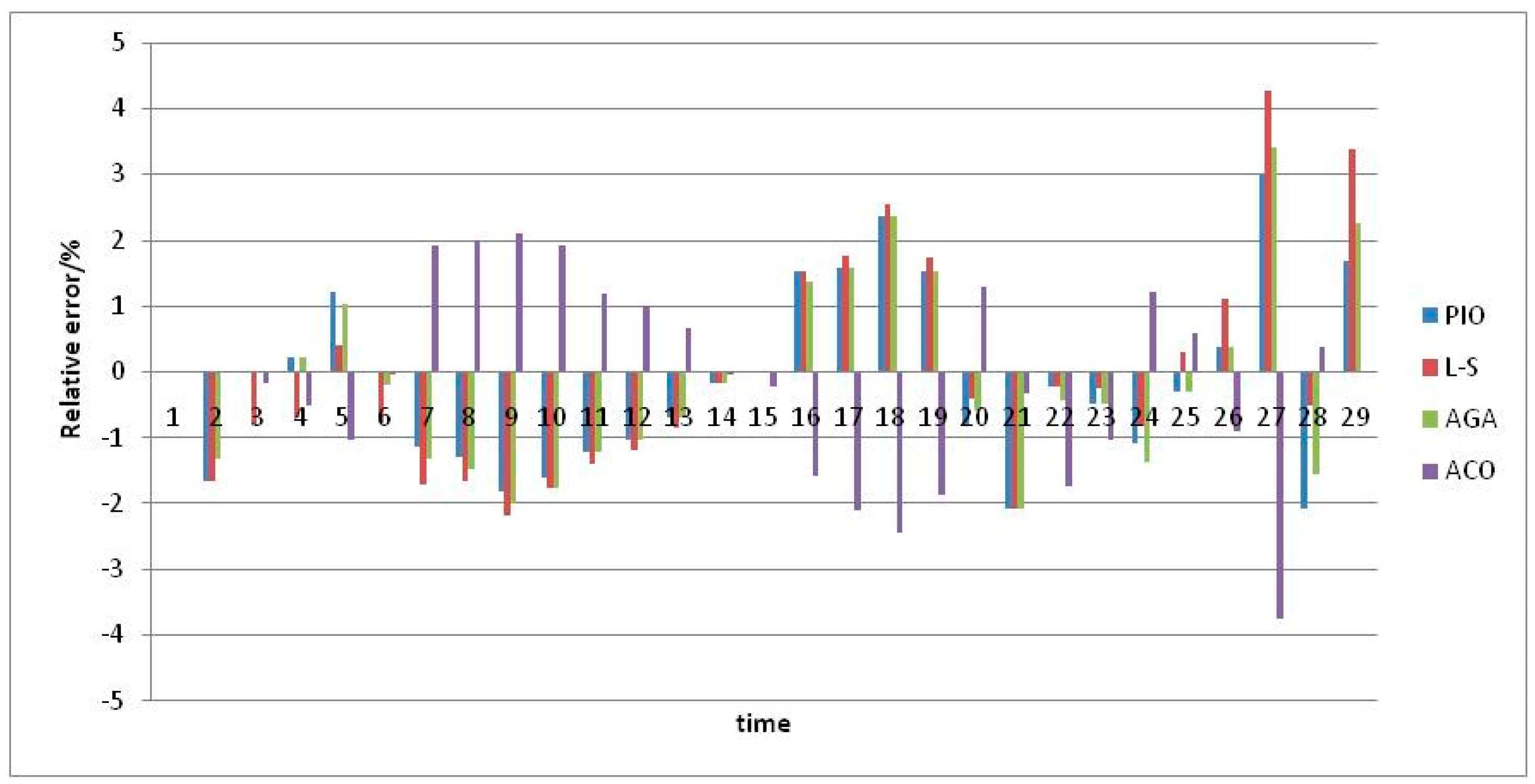
The relative error of the simulated results obtained from the four algorithms is shown in Figure 2, as calculated by:
The simulation results of four algorithms are shown in Figure 3. As shown in Figure 3, the PIO algorithm performs well in terms of solving the parameter estimation problem of the Muskingum model. The parameter estimation results of the four algorithms, their average absolute error, and the average relative error among their simulation results are shown in Table 1.
The PIO algorithm results have the lowest average absolute error and average relative error, i.e., PIO possesses better solution accuracy and better optimization performance than the three other algorithms we tested. Also, its computational time was 1.625 s. Thus, the PIO algorithm is an excellent approach to solving the Muskingum model parameter estimation problem.
2.3. “In-Process Type” Dynamic Parameter Estimation of the Muskingum Model Based on BP-Neural Network
2.3.1. Basic Principles of BP-Neural Network
The artificial neural network is a simulation of human physiological structures and mechanisms which depart from symbolic reasoning or logical thinking [30,31]. It plays a role in mitigating imperfect associative memory, defective feature pattern recognition, automatic rule-learning, and other functions. It plays an especially crucial role in solving complex problems [32,33,34] which are difficult to model, such as the computer-aided molecular design problem [32], spatial distribution of soil heavy metals problem [33], and modulation transfer function estimation problem [34].
The Back-Propagation (BP) Neural Network is one of the most commonly used neural network models. The research group led by Rumelhart and McClelland [35] analyzed the error back-propagation algorithm of multilayer feed-forward networks, which possess a nonlinear continuous transfer function, in the book Parallel Distributed Processing. The basic idea of the BP algorithm is that the learning process consists of two processes: forward propagation of signal and backward propagation of error. In the process of forward propagation, the input samples are imported from the input layer and then transmitted to the output layer after being processed in the hidden layer. If the errors between actual outputs of the output layer and the expected outputs do not meet the requirements, they then transfer to the error backward propagation. The error back-propagation is used to transfer the output errors to the input layer through the hidden layer, and then apportion the error to all the units of each layer in order to obtain the error signal of each unit, which is the basis for correcting each unit. The process of adjusting the weight of each layer in signal forward-propagation and error back-propagation goes on again and again, and the procedure of weight adjustment is the so-called learning and training process of the network. This process will not stop until the error of the network output is reduced to an acceptable level or to the preset number of studies.
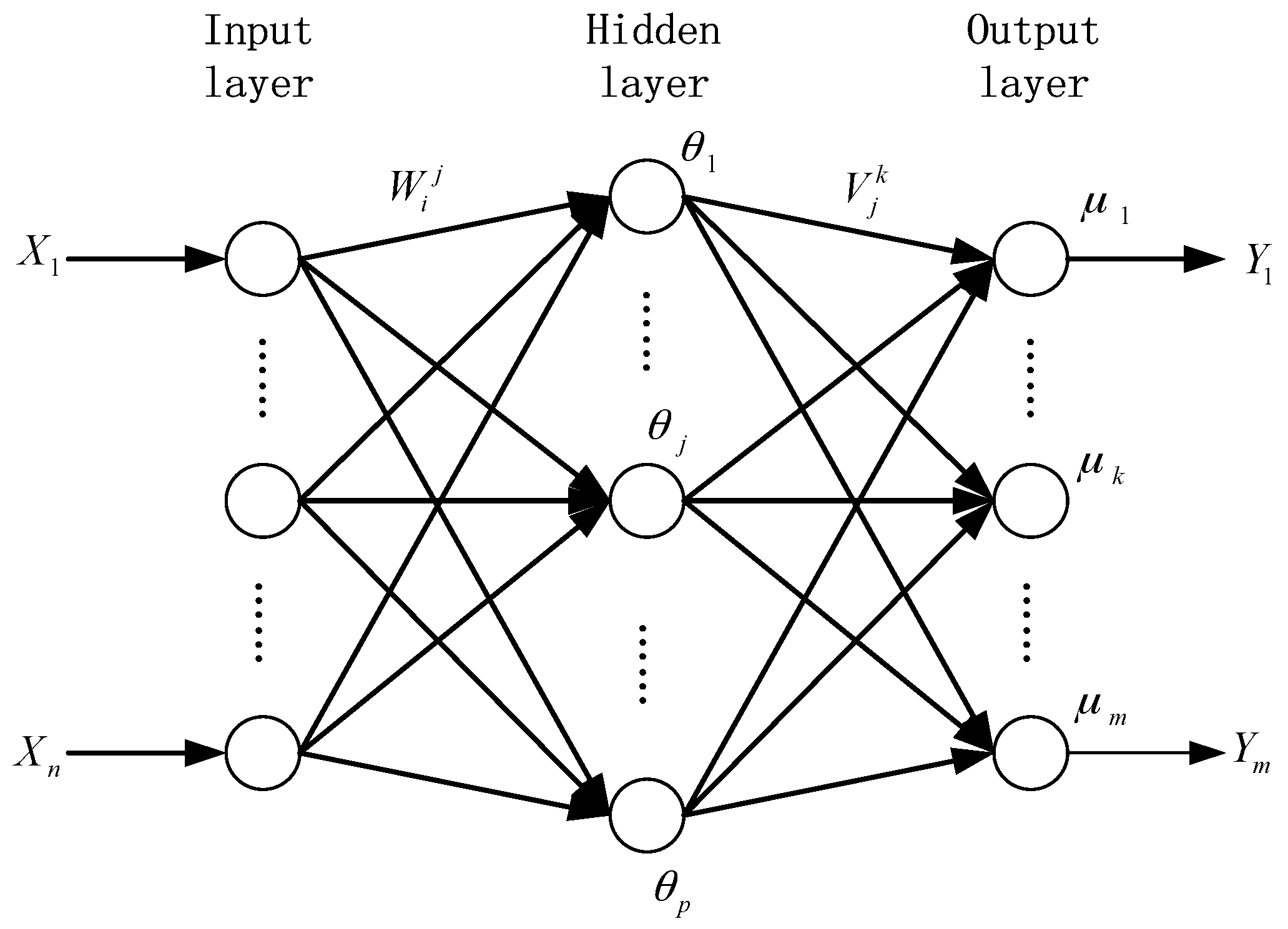
Its advantages include: (1) a simple structure and strong operability; (2) nonlinear mapping from input to output, which realizes any complex nonlinear mapping; and (3) strong self-learning and summarization abilities [36]. We selected a three-layer BP network for dynamic Muskingum model parameter estimation. The three layer BP network topology is shown in Figure 4.
The network contains an input layer, a hidden layer, and an output layer, and the learning procedure of the BP-ANN model is shown as below.
- Step 1
- Network initialization. The number of node in the input layer is n, in the hidden layer is p, and in the output layer the node number is m. The connection weights between the input layer and the hidden layer, the hidden layer and the output layer is and , respectively. The threshold of hidden layer is and the threshold of output layer is
- Step 2
- Calculate the output of hidden layer. The calculation formula is:where is the excitation function of hidden layer, and is the input of node i.
- Step 3
- Calculate the output of output layer. It is calculated by
- Step 4
- Update the weights through the equations as follows:where is the learning rate and , , , and is momentum factor and .
- Step 5
- Threshold update. Update the value of and according to the error between the network output and the desired output . The formulas to calculate and are:
- Step 6
- Determine whether the iteration ends. If it doesn’t end, go back to step 2.
2.3.2. Basic Theory of “In-Process Type” Dynamic Parameter Estimation
As discussed above, the Muskingum model has continually increased in popularity since its proposal in 1938; the most important function of the model is the selection of parameters K and x. Hydrologists such as Xu et al. [16,18,37] have taken a single set of parameters as the Muskingum model parameters in one river channel, which can be determined by the estimation of one of the floods or the mean estimated value of multiple floods. Modern optimization algorithms, as opposed to traditional methods like trial-and error, have contributed substantially to the development of today’s single-flood parameter estimation models. However, a river with only a single set of model parameters does not readily satisfy the application requirements [9].
Thus, Liang [38] proposed that the parameter K should be determined by the flow classification method—that is to say, the peak discharge with varying magnitudes should adopt different K values while the parameter x is still determined by the estimated mean. Although this remedies the application defect of a single parameter set to some extent, the problem remains fundamentally unresolved due to the large nonlinearity between the peak discharge and the values of K and x. We suggest that the flood model parameters should be determined by the specific flood condition, and that real-time dynamic parameter estimation of the Muskingum model for river course flood should also be realized.
Most of the commonly used Muskingum model parameter estimation methods are “posterior type” [9], where flood parameters are estimated via simulation of floods which have already occurred. Of course, the accuracy of this type of flood simulation is generally high, but the actual forecast may have insufficient accuracy even when the parameter accuracy of the posterior estimation is sufficient. Each flood has its own characteristics, which causes variations in the model parameters (or sometimes even markedly diverge them). The “in-process type” parameter estimation method better accounts for this; it estimates parameters while a flood is occurring, then assigns a set of unique parameter sets to the flood.
As to the real-time flood forecasting, it corrects the results and parameters in the process of model prediction. The research of real-time flood forecasting was carried out earlier, and Japanese scholar M. Hino [39,40] proposed that the method of Kalman Filter could be applied to hydrological forecasting, and he developed it in his later papers in 1973. And Todini [41], a professor of University of Bologna in Italy, established the mutually interactive state-parameter (MISP) algorithm in 1978, becoming the first-generation real-time flood forecasting model. Kleanidis and Bras [42] improved the Sacramento model in 1980, realizing real-time prediction through the application of the Kalman filtering model. In 1987, Georgakakos [43] presented a stochastic and dynamic meteorological and hydrological forecast model.
In 1995, Song [44] first introduced and improved the method of recursive least-squares parameter identification raised by T.R. Fortesuce et al., based on variable forgetting factors, which provided a powerful tool for parameter identification of real-time flood forecasting model. Then, in 1995, Zhong et al. [45] tried to introduce artificial neural network technology into real-time flood forecasting. In 1996, Guo et al. [46] developed an integrated automation system of reservoir operation for the Tuo Xi hydropower station in Hunan. From then on, a decision support system for real-time flood forecasting, flood control, and power generation dispatching had been developed, and the automation of forecast dispatching had also been realized. In 2011, Luo et al. [9] thought that floods from the same river should have different parameters, and presented the Muskingum model with adaptive parameter using the time series similarity search method. However, this article also has some shortcomings; only after the flood from upstream has finished can the parameters be obtained, thus the forecast period of the flood is shortened. From this point of view, this paper puts forward the research idea.
In this study, based on the previous single-flood parameter estimation method in Section 2.2.2, we first estimated the flood parameter and extracted the characteristic attributes of several floods, then took these attributes as inputs and flood parameters as the outputs to train the BP-ANN model. After that, if we could obtain the attributes of the happening flood, then the flood parameters could also be obtained from the BP-ANN model. Thus, the Muskingum model parameters could be dynamically estimated in real-time. The proposed method was implemented as follows.
- Step 1
- Select multiple floods and use the PIO algorithm to estimate their respective parameters.
- Step 2
- Extract the characteristic attributes of each flood according to the specific river conditions.
- Step 3
- Take the extracted characteristic attributes of each flood as the input, and parameters and of the Muskingum model as outputs to train the Neural Network model; use the PIO algorithm to estimate the parameters.
- Step 4
- Extract the characteristic attributes of the flood to be forecasted and plug them into the Neural Network to calculate parameters and of the Muskingum model, then use the Muskingum model to perform the flood routing computation.
The Neural Network model is not invariable once it has been established. New data should be updated into the database and the model continually trained to improve its prediction accuracy.
2.3.3. Study River Channel
The Yellow River is located in Northern China. It has a total length of 5464 km and its basin covers 752,443 km2, making it the fifth longest river in the world and the second longest river in China. The annual precipitation in most parts of the Yellow River Basin is about 200 to 650 mm, and the annual precipitation in the lower reach is more than 650 mm. The Sunkou and Gaocun Hydrometric Stations, which are the national key hydrometric stations in the lower reaches of the Yellow River, are located in Shandong Province. There are about 197 km between the two hydrometric stations, in which there are no tributary imports or exports. We selected this river channel to validate the proposed dynamic parameter estimation method of the Muskingum model (Figure 5).
2.3.4. Extracting Flood Characteristic Attributes
There are several characteristic attributes that influence flood routing processes, including antecedent rainfall, soil moisture content, water level, flow velocity, and peak discharge. We analyzed the 60 floods which occurred over the past 40 years according to the Gaocun and Sunkou Hydrometric Stations, and we found that it takes about 6–65 h for the flood routing from Gaocun to Sunkou; a single flood in this portion of the Yellow River lasts for about 5–36 days. After a comprehensive analysis, we extracted the following characteristic attributes of the floods in this river reach via the proposed “in-process type” estimation method, which can be shown in Figure 6:
- (1)
- The initial water level (IWL), which corresponds to the rising point (the time at ) of the flood, reflects the rising conditions of the flood and the previous water volume of the river. The larger the previous water volume, the more prone the area of interest is to flooding. The water level also reflects flow velocity information and thus exerts some influence on flood routing.
- (2)
- The peak discharge (PD), which reflects the magnitude of the flood and has significant influence on flood routing.
- (3)
- The flood peak emergence time (FPET), i.e., the time at which the flood appears. FPET is usually an instantaneous value, so it cannot exactly reflect the characteristics of each flood along the entire route. Here, we consider the point at which the flood peak appears as the FPET; that is to say, , in which T is the duration time of the flood.
- (4)
- The total flood volume on the first two days after a flood appears (FVFT) reflects the rising conditions of the flood.
- (5)
- The flood volume on the day before the flood peak appears (FVBFP), which reflects the width of the flood peak.
- (6)
- The average discharge before the flood peak (ADBFP), i.e., the mean discharge prior to the flood peak, which reflects the ratio between the total flood volume and time.
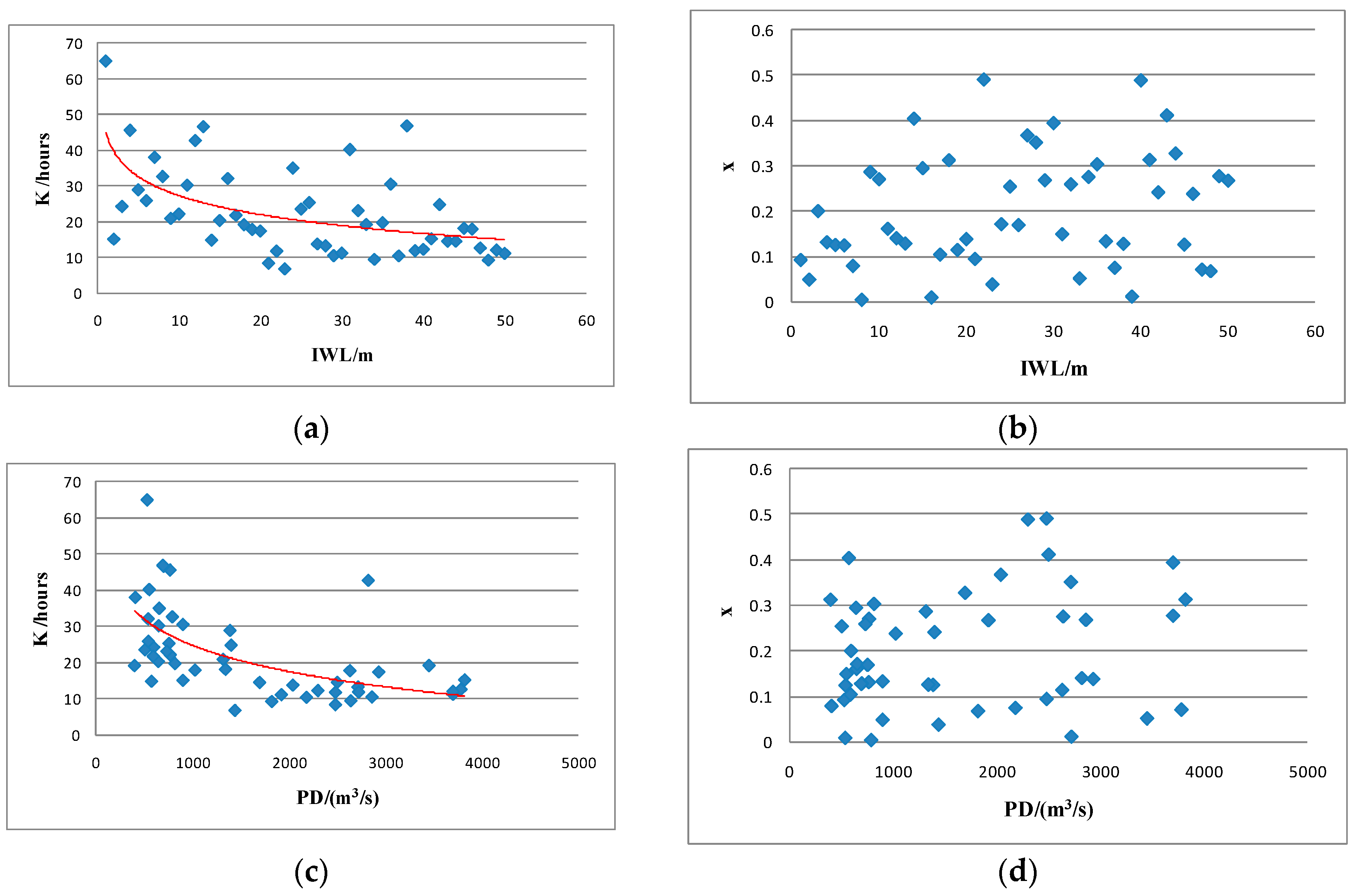
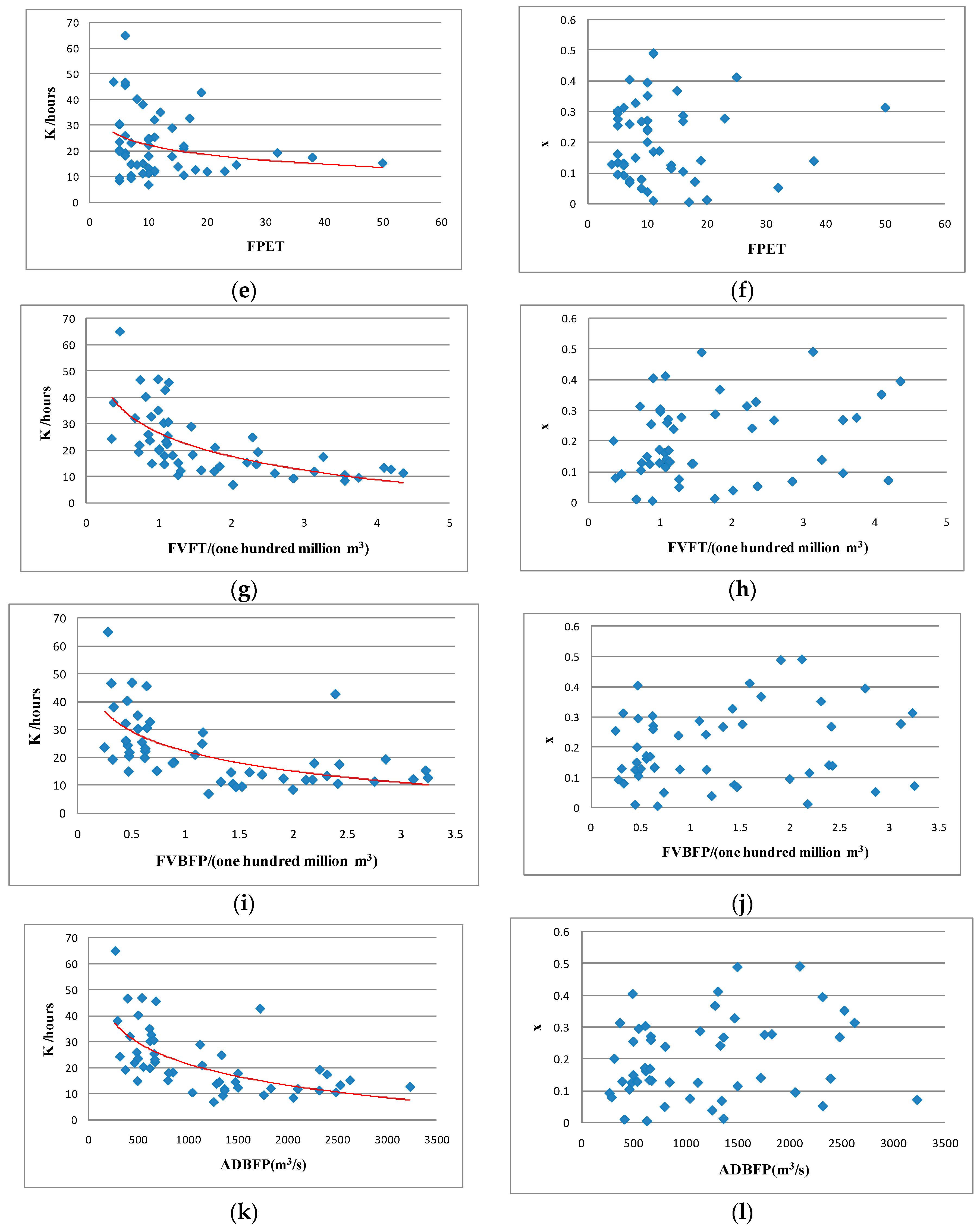
Based on the first 50 floods in our dataset, we used the PIO algorithm to estimate the Muskingum model parameters. We used the same PIO parameters as those defined in Section 2.2.2 and calculation period , then as to each flood, we ran the algorithm five times to obtain five results of the parameter to make sure that the results are believable. We took the optimum of the objective function as the parameter estimation result. The last ten floods were used to validate the constructed dynamic parameter estimation model, while PIO was used to estimate parameters K and x. We can obtain the correlation between the characteristic attributes and K and x, as shown in Figure 7, according to the pre-extracted characteristic attributes of each flood.
Figure 7a,c,e,g,i,k indicate that the value of parameter K varies from 5 to 65. K decreases as the value of each characteristic attribute increases; it has a large variation range. These results suggest that error is inevitable regardless of whether the mean K value or the K value in accordance with the peak discharge magnitude is utilized.
As shown in Figure 7b,d,f,h,j,l, the value of parameter x fluctuates between 0 and 0.5; in other words, it fluctuates considerably as each characteristic attribute increases in value. We found no obvious change trend in x. To this effect, substituting the mean value of x into the Muskingum model will cause an error.
2.3.5. The Flow Chart of the IP-DPE Method
To clearly explain the process of the proposed IP-DPE method, we provide a flow chart as Figure 8.
3. Results
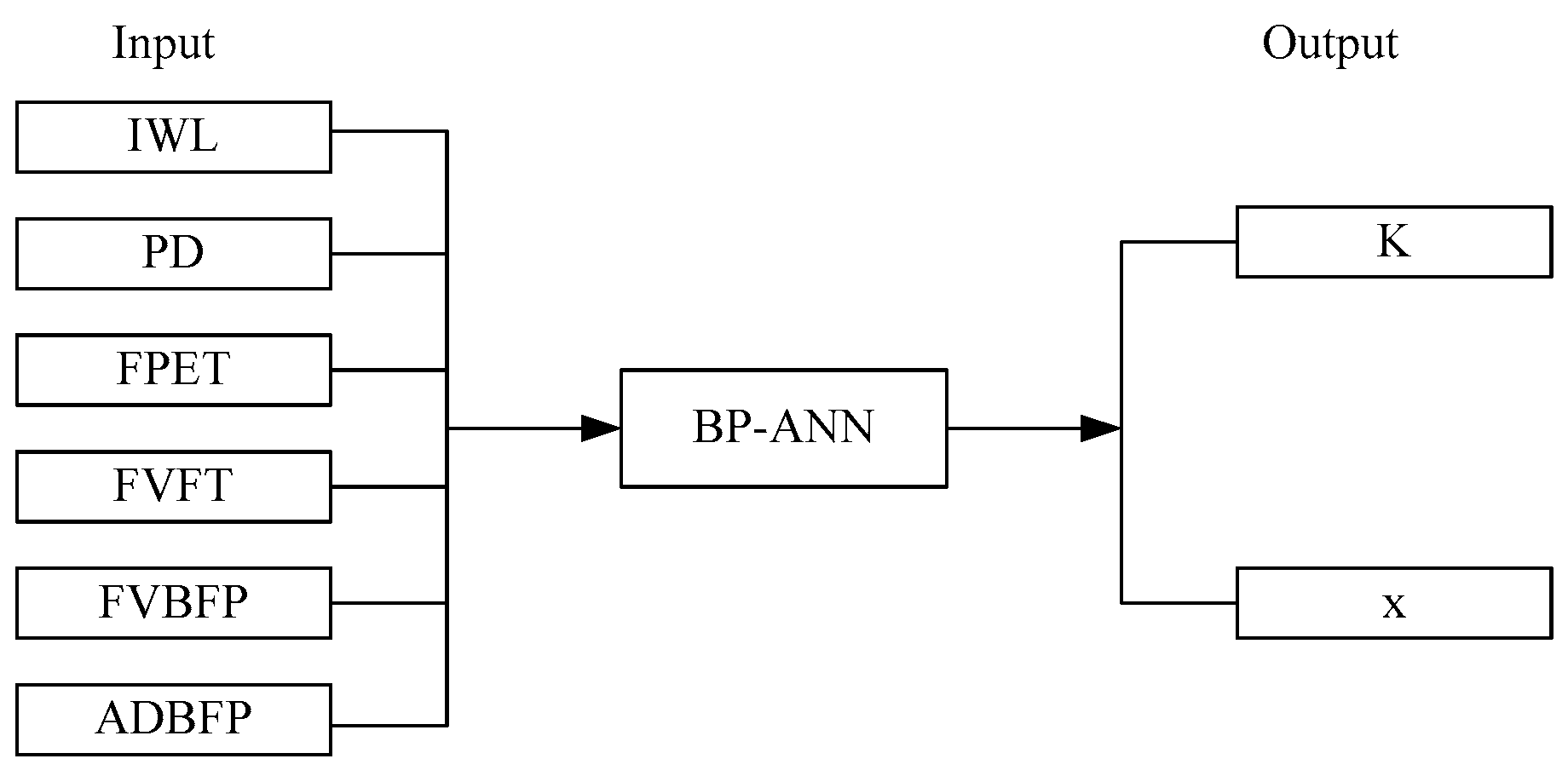
We established the dynamic parameter estimation method of the Muskingum model based on the BP-Neural Network, as discussed above. The characteristic attributes of each flood were input to the model. The input layer of the Neural Network has six nodes, the hidden layer has five nodes, and the outputs of the Neural Network are the Muskingum model parameters K and x—this comprises the “6-5-2 type” BP-Neural Network model. There are 42 parameters in the Neural Network model, as established. Because the traditional Newton Iteration and Gradient methods easily fall into local optima [47,48], we used the PIO algorithm to realize parameter estimation in the Neural Network model, using the same parameters referred to above. The structure diagram of the resulting BP-Neural Network is shown in Figure 8.
The first 50 floods were substituted into the Neural Network to train the model, and the last 10 floods were used to verify the model. We also ran the traditional Muskingum model parameter optimization methods, mean value (MV) method, and flow classification (FC) method for comparison against the proposed “in-process type” dynamic parameter estimation (IP-DPE) method. According to the Standard for Hydrological Information and Hydrological Forecasting (SL 250-2000), we used the following three indexes to evaluate the results.
- (1)
- The mean absolute error (MAE) of the flood (m3/s):where T is the duration of the flood, is the observed flow of the flood at time i, and is the calculated flow of the flood at time i.
- (2)
- The average relative error (ARE) of the flood (%):
- (3)
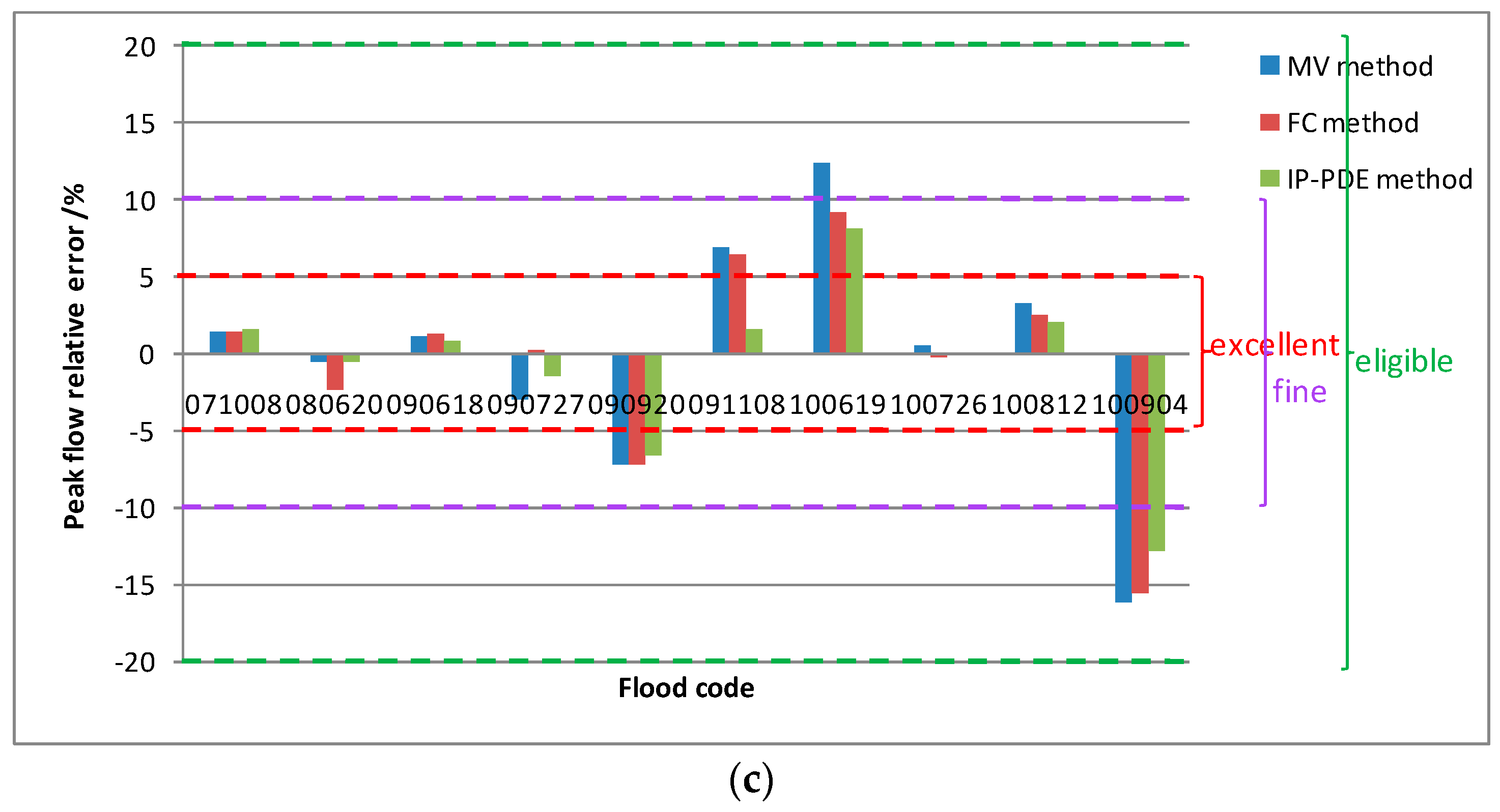
- The peak flow relative error (PFRE) of the flood (%):where represents the observed peak flow of the flood and is the calculated peak flow of the flood. The evaluation results are shown in Table 2.
The simulated performance of the three methods is shown in Figure 9.
As shown in Table 2 and Figure 9, the flood forecasting results obtained from the three methods are all technically reasonable but do show marked differences in forecasting accuracy. The MAE value can well reflect the actual prediction error without the positive and negative values cancellation. Nine of the optimal MAE values of floods were obtained from the IP-DPE method, and one optimum was obtained from the FC method. The MV method had the worst estimation results of six floods, and the simulated MAE of flood No. 090618 was almost three times that of IP-DPE method. The MAE range of the MV method was 16.177–216.32, that of the FC method was 16.294–160.83, and that of the IP-DPE method was 15.765–153.97. The IP-DPE method had the least fluctuation range and the error is generally low; in other words, IP-DPE had smaller fluctuations and was more stable than the other methods, and the MV method had the worst performance.
The ARE value can reflect the overall situation of the prediction error; nine optimal ARE values were obtained from the IP-DPE method and one optimal from the FC method. Seven of the MV method forecast results were the worst, and the simulated ARE of flood No. 091108 was nearly two times that of the IP-DPE method. The three floods estimated by the MV method fluctuated by more than 10% in ARE, and one flood estimated by the FC method exceeded 10%. The ten floods estimated by the IP-DPE method fluctuated less than 9% in ARE values, again indicating that the proposed method has more stable performance.
Eight optimal PFRE values were obtained from the IP-DPE method. The estimation error of MV and FC methods for flood No. 100904 both exceeded 15%, indicating that their peak flow forecasting performance is poor. The IP-DPE method also has the optimal fluctuation range among them.
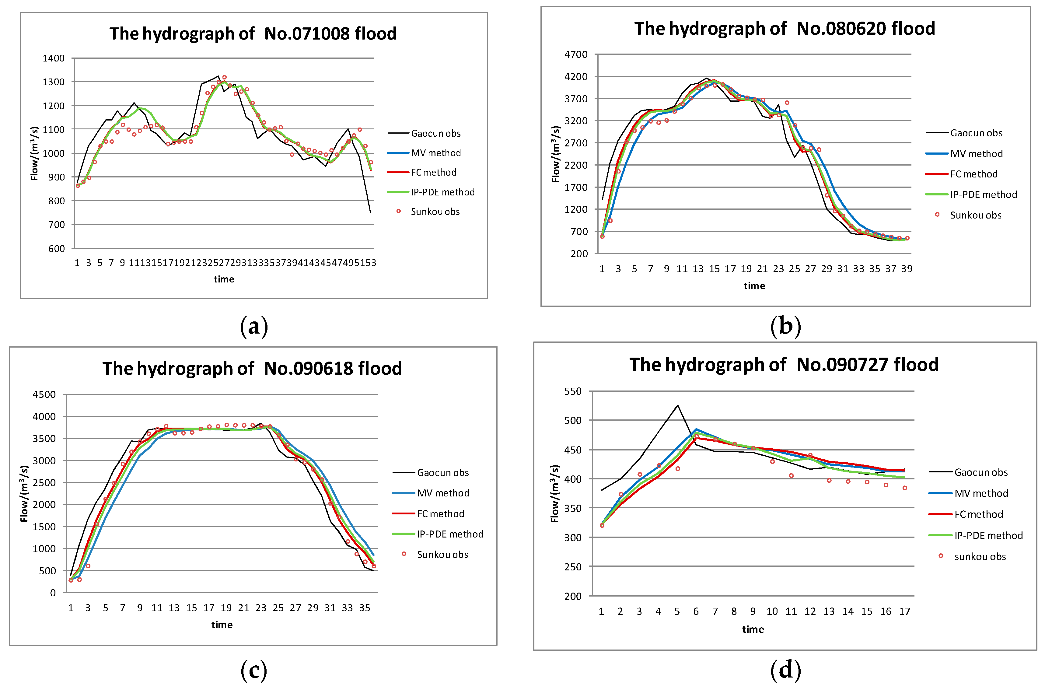
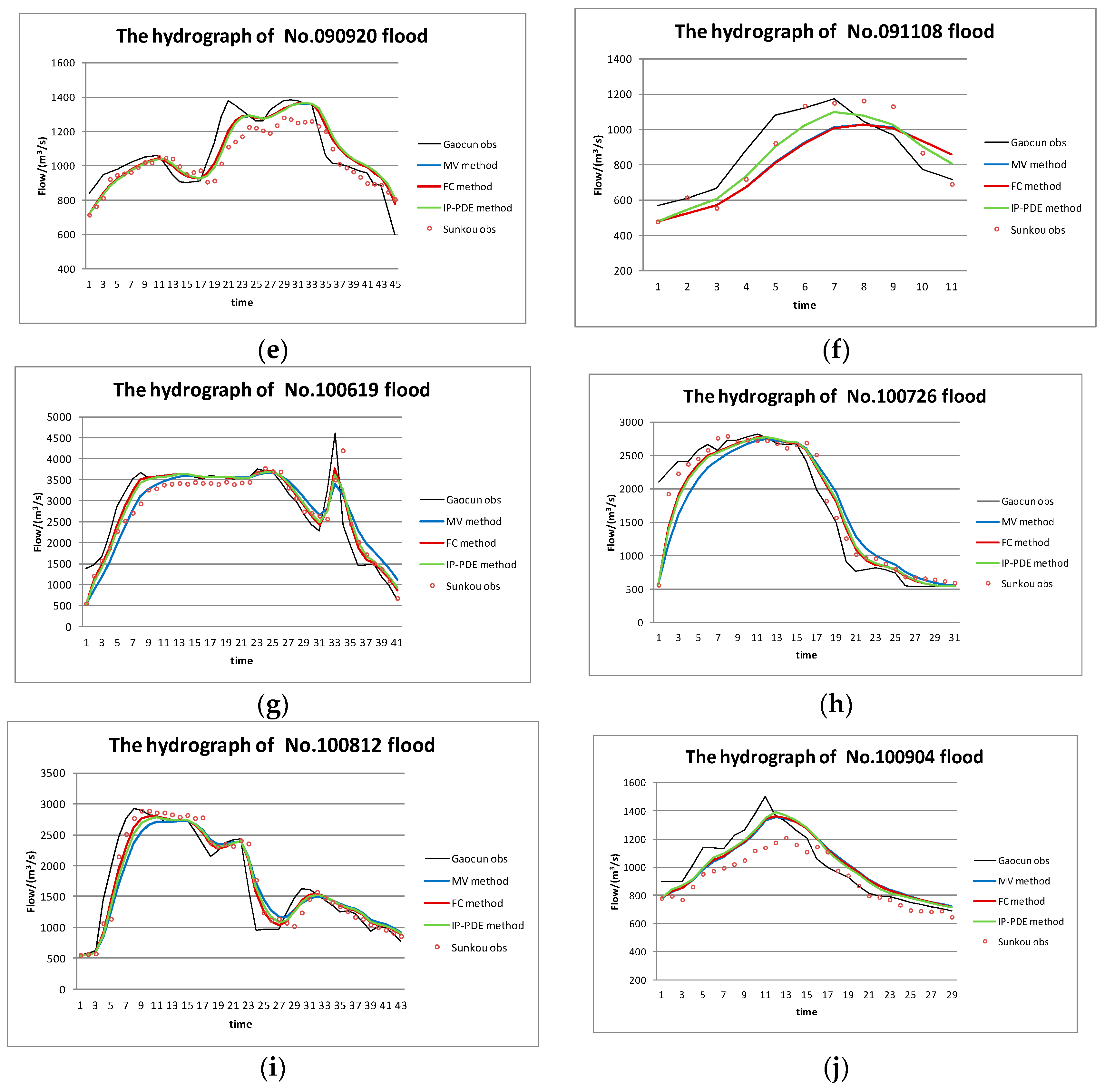
A comparison among the prediction results of the three methods is shown in Figure 10. “Gaocun obs” refers to the observed values of Gaocun Hydrometric Station, while “Sunkou obs” refers to those of the Sunkou Hydrometric Station.
Our results indicate that the IP-DPE method had the best performance and the MV method had the poorest performance of the three methods we tested.
From Figure 11, we can find that the flood has moderate attenuation from the upstream section to the downstream section, especially the decreases of flood peak and when the flood peak becomes chunky. In this regard, Zhang et al. [49] believe that if there is no bed scouring and siltation in the river channel, and the shapes of cross-sections are unchanged along the channel, the flow is assumed as clear water. Under the circumstance of constant roughness, the flood peak discharge attenuates and peak pattern grows chunky along the river because of the influence of the channel storage and side wall resistance. In the case that roughness decreases with time and the reduction rate of the upper reaches is greater than that of the lower reaches, the discharge increases abnormally along the river channel. In addition, the greater the reduction rate, the more obvious the peak increase. In this paper, we use the Muskingum model to carry out our research from the hydrological point of view. These effects have all been included in the model parameters, and the floods evolved by these parameters also verify this phenomenon.
4. Discussion
Theoretically, for the same river channel, we can suppose that the values K and x are constant in the linear Muskingum model. In practice, however, the factors that impact the flood forecasting accuracy may contain the uncertainty of data; the rainfall conditions before the flood, runoff in the river channel, flood magnitude, and discharge hydrograph vary under so many influence factors that using one group of parameters in the same river channel is no longer applicable. Although the factors that cause the forecasting errors may be known, it is quite difficult to analyze their exact influence or the exact extent of said influence. We use the Neural Network black-box model to synthesize the characteristic attributes of the flood to output the necessary parameters in such a way that these influence factors are minimized.
We can see from Figure 11, in the process of validation, that there is a small part of floods presenting inaccurate forecasts of peak timing. After the analysis, we found that the inaccurate results mainly appear in the prediction of multi-peak floods, and there is a tiny fluctuation near some parts of the flood peaks of the multi-peak flood. However, in the course of flood routing, the next period data was obtained by superimposing the data of the previous period with the data of this period. Therefore, it is possible that the peak timing is not completely consistent after the superposition of the current and the previous period. Although there are errors between the actual values and the predicted values, the errors are very small and will almost not affect the flood forecast.
Though the results obtained through the proposed method are more accurate than through the traditional method, IP-DPE is not perfect. For example, the model can only accurately reflect floods with the specific characteristic attributes that are substituted into it. The same attributes may not be available for a model of a different river channel. Although the current simulation accuracy is higher than the other methods, some of the flood characteristics are made available very close the flood peak, and there may also be altogether better attributes than those we used in this study. We plan to continue researching IP-DPE using other river channels as case studies and with different characteristic attributes for parameter estimation in order to continue improving the model’s efficiency and efficacy.
5. Conclusions
In researching the more commonly used Muskingum model parameter estimation methods, we observed a tendency to set parameters according to mean values or flow magnitude, in which the practicability of the model and the applicability of the parameter are not fully considered. We assert that because each flood has its own particular parameters, that an “in-process type” dynamic parameter estimation method based on the PIO algorithm and BP-Artificial Neural Network model is the better choice for building a highly accurate Muskingum model.
After a brief literature review, we established the proposed Muskingum model parameter optimization model via the PIO algorithm. We then used data of floods occurring in the river channel from Chenggouwan to Linqing of Haihe River Basin in the year 1961 as an example and ran the PIO algorithm, L-S method, AGA method, and ACO algorithm to estimate Muskingum model parameters to validate the applicability and excellent performance of the PIO algorithm by comparison among them.
We also proposed the “in-process type” dynamic parameter estimation method for the Muskingum model based on the BP-Artificial Neural Network. According to the single-flood parameter estimation results, we extracted six characteristic attributes of each flood: IWL, PD, FPET, FVFT, FVBFP, and ADBFP, which were taken as input to obtain Muskingum model parameters K and x, which we used to establish the BP-ANN model.
We next took a channel of the Yellow River from Sunkou Hydrometric Station to Gaocun Hydrometric Station as a case study. We selected 60 floods which occurred over the past 40 years for analysis and applied the PIO algorithm to estimate the Muskingum model parameters of each flood. These results were used to obtain the correlation between the characteristic attributes and parameters K and x. We found that K decreases nonlinearly as each characteristic attribute increases, while x has a larger fluctuation range with no obvious rule. Therefore, if we select the mean parameter values, or take the parameter values in accordance with peak discharge magnitude as the input of the river flood forecasting model, it will cause an error.
Finally, we established IP-DPE for the Muskingum model based on the “6-5-2 type” BP-Artificial Neural Network. We used the first 50 floods from the dataset for model training and the last ten for validation. We also ran the MV and FC parameter estimation methods for performance comparison. We took the average absolute error, average relative error, and peak flow relative error as evaluation criteria to evaluate the simulation performance of the three methods and give out the flood simulation results of the last ten floods. The results showed that the proposed IP-DPE method had the most satisfying simulation results and best performance.
Acknowledgments
This work was supported by the National Key Research and Development Program of China (2016YFC0401409), the National Natural Science Foundation of China under Grant No. 51507141, and the special scientific research plan project of Shaanxi Province Education Office (17JK0547).
Author Contributions
Gang Zhang and Tuo Xie conceived and designed the experiments. Gang Zhang, Lei Zhang, and Bin Zhao performed the experiments. Tuo Xie, Lei Zhang, Xi Chen, and Fangfeng Li analyzed the data. Gang Zhang and Xia Hua contributed reagents/materials/analysis tools. Gang Zhang, Xia Hua, and Lei Zhang wrote the paper. Gang Zhang, Lei Zhang, and Chen Wu translated and revised the paper.
Conflicts of Interest
The authors declare no conflict of interest.
References
- Vijay, P.S.; Roger, C.M. Some notes on Muskingum method of flood routing. J. Hydrol. 1980, 48, 343–361. [Google Scholar]
- Kumar, D.N.; Baliarsingh, F.; Raju, K.S. Extended Muskingum method for flood routing. J. Hydro-Environ. Res. 2011, 5, 127–135. [Google Scholar] [CrossRef]
- Wang, G.S.; Ning, G.F.; Xiao, F. Practical Hydrological Forecasting Methods; Water Power Press: Beijing, China, 2008. [Google Scholar]
- Gill, M.A. Flood routing by the Muskingum method. J. Hydrol. 1978, 36, 353–363. [Google Scholar] [CrossRef]
- O’Donnell, T. A direct three-parameter Muskingum procedure incorporating lateral inflow. Hydrol. Sci. J. 1985, 30, 479–496. [Google Scholar] [CrossRef]
- Aldama, A.A. Least-squares parameter estimation for Muskingum routing. J. Hydraul. Eng. 1990, 116, 580–586. [Google Scholar] [CrossRef]
- Kshirsagar, M.M.; Rajagopalan, B.; Lal, U. Optimal parameter estimation for Muskingum routing with ungauged lateral inflow. J. Hydrol. 1995, 169, 25–35. [Google Scholar] [CrossRef]
- Yoon, J.; Padmanabhan, G. Parameter estimation of linear and nonlinear Muskingum models. J. Water Resour. Plan. Manag. 1993, 119, 600–610. [Google Scholar] [CrossRef]
- Luo, J.G.; Xie, J.C.; Zhang, G. Parameter adaptive Muskingum method of flood routing. J. Hydroelectr. Eng. 2011, 30, 57–64. [Google Scholar]
- Chen, J.J.; Yang, X.H. Optimal parameter estimation for Muskingum model based on Gray-encoded accelerating genetic algorithm. Commun. Nonlinear Sci. Numer. Simul. 2007, 12, 849–858. [Google Scholar] [CrossRef]
- Cheng, C.T.; Ou, C.P.; Chau, K.W. Combining a fuzzy optimal model with a genetic algorithm to solve multi-objective rainfall-runoff model calibration. J. Hydrol. 2002, 268, 72–86. [Google Scholar] [CrossRef]
- Moghaddam, A.; Behmanesh, J.; Farsijiani, A. Parameters Estimation for the New Four-Parameter Nonlinear Muskingum Model Using the Particle Swarm Optimization. Water Resour. Manag. 2016, 30, 2143–2160. [Google Scholar] [CrossRef]
- Ouyang, A.J.; Li, K.L.; Tung, K.T.; Sallam, A.; Sha, E.H.-M. Hybrid particle swarm optimization for parameter estimation of Muskingum model. Neural Comput. Appl. 2014, 25, 1785–1799. [Google Scholar] [CrossRef]
- Shao, N.H.; Shen, B. Application of Chaotic Particle Swarm Optimization to Parameter Estimation in Mustingum Model. J. Water Resour. Water Eng. 2009, 20, 30–33. [Google Scholar]
- Zhan, S.C.; Xu, J. Application of ant colony algorithm to parameter estimation of muskingum routing model. J. Nat. Disasters 2005, 14, 20–24. [Google Scholar]
- Xu, D.M.; Qiu, L.; Wang, W.C. Effective parameter estimation of Muskingum model based on the SCE-UA algorithm. Yellow River 2008, 30, 31–35. [Google Scholar]
- Lu, F.; Jiang, Y.Z.; Wang, H.; Niu, C.W. Application of multi-agent genetic algorithm to parameter estimation of Muskingum Model. J. Hydraul. Eng. 2007, 38, 289–294. [Google Scholar]
- Song, W.Z.; Lei, X.H.; Huang, X.M.; Tang, B.; Jiang, Y.Z. Application of multi-objective Particle Swarm Optimization in Muskingum parameter estimation considering crowding distance. Water Resour. Power 2013, 31, 38–41. [Google Scholar]
- Wang, H.X.; Zhang, C.; Dong, S.H. Variable parameters of Muskingum model for flood routing. Water Resour. Power 2012, 30, 47–49. [Google Scholar]
- Hostache, R.; Matgen, P.; Schumann, G.; Puech, C.; Hoffmann, L.; Pfister, L. Water level estimation and reduction of hydraulic model calibration uncertainties using satellite SAR images of floods. IEEE Trans. Geosci. Remote Sens. 2009, 47, 431–441. [Google Scholar] [CrossRef]
- Ye, S.Z.; Zhan, D.J. Engineering Hydrology; China Water & Power Press: Beijing, China, 1999. [Google Scholar]
- Lin, S.Y. Hydrologic Forecasting; China Water & Power Press: Beijing, China, 2001. [Google Scholar]
- Li, M.M.; Li, C.J.; Zhang, M. The application of improved PSO algorithm in the parameter estimation of Muskingum model. Yangtze River 2008, 39, 60–61. [Google Scholar]
- Duan, H.B.; Qiao, P.X. Pigeon-inspired optimization: A new swarm intelligence optimizer for air robot path planning. Int. J. Intell. Comput. Cybern. 2014, 7, 24–37. [Google Scholar] [CrossRef]
- Guilford, T.; Robert, S.; Biro, D.; Rezek, I. Positional entropy during pigeon homing II: Navigational interpretation of Bayesian latent state models. J. Theor. Biol. 2004, 227, 25–38. [Google Scholar] [CrossRef] [PubMed]
- Whiten, A. Operant study of sun altitude and pigeon navigation. Nature 1972, 237, 405–406. [Google Scholar] [CrossRef]
- Duan, H.B.; Ye, F. Progresses in pigeon-inspired optimization algorithms. J. Beijing Univ. Technol. 2017, 43, 1–7. [Google Scholar]
- Yangzhou Water Conservancy Institute. Hydrologic Forecasting; China Water & Power Press: Beijing, China, 1979. [Google Scholar]
- Yang, X.H.; Jin, J.L.; Chen, Z.S.; Wei, Y.M.; Tan, J.W. A new approach for parameter estimation of Muskingum routing model. J. Catastrophol. 1998, 13, 1–6. [Google Scholar]
- Li, X.Y.; Cheng, C.T.; Lin, J.Y. Bayesian probabilistic forecasting model based on BP ANN. J. Hydraul. Eng. 2006, 37, 354–359. [Google Scholar]
- Kalteh, A.M. Monthly river flow forecasting using artificial neural network and support vector regression models coupled with wavelet transform. Comput. Geosci. 2013, 54, 1–8. [Google Scholar] [CrossRef]
- Zhou, X.; He, X.R.; Chen, B.Z.; Qiu, T. Computer-aided molecular design with BP-ANN and global optimization algorithm. Comput. Aided Chem. Eng. 2003, 15, 690–695. [Google Scholar]
- Li, Y.; Li, C.K.; Tao, J.J.; Wang, L.D. Study on spatial distribution of soil heavy metals in Huizhou City based on BP-ANN modeling and GIS. Procedia Environ. Sci. 2011, 10, 1953–1960. [Google Scholar] [CrossRef]
- Gu, Y.Y.; Shen, X.H.; He, G.X. MTF estimation via BP neural networks and Markov model for space optical camera. J. Frankl. Inst. 2013, 350, 3100–3115. [Google Scholar] [CrossRef]
- James, L.M.; David, E.R.; The PDP Research Group. Parallel Distributed Processing; The MIT Press: Cambridge, UK, 1987. [Google Scholar]
- Zhang, D.F. Evaluation of sustainable use of water resources in Wenshan based on AHP-BP model. J. Water Resour. Water Eng. 2013, 24, 203–209. [Google Scholar]
- Cheng, Y.C.; Zuo, X. Parameter estimation method of nonlinear Muskingum model based on Chaos-simulated annerling method. J. Shandong Agric. Univ. 2006, 37, 235–239. [Google Scholar]
- Liang, H. The Research of Parameter and the Optimal Parameters’ Estimation Method of Muskingum Model for River Flood Routing; Guangxi University: Nanning, China, 2015. [Google Scholar]
- Hino, M. Runoff forcasts by linear predictive filter. J. Hydraul. Div. 1970, 96, 681–701. [Google Scholar]
- Hino, M. On-line prediction of a hydrologic System. In Proceedings of the 15th IAHR Congress, Istanbul, Turkey, 1973. [Google Scholar]
- Todini, E. Mutually interactive state-parameter estimation. In Proceedings of the American Geophysical Union Chapman Conference on Application of Kalman Filtering Theory and Techniques to Hydrology, Hydraulics and Water Resources, Pittsburgh, PA, USA, May 1978; Volume 5. [Google Scholar]
- Kidanidis, P.K.; Bras, R.L. Real-time forecasting with a conceptual hydrologic model [(1) Anaiysls of UnCertainty; (2) Application and results]. Water Resour. Res. 1980, 16, 1025–1033. [Google Scholar] [CrossRef]
- Georgakakos, K.P. Real-time flash flood prediction. J. Geophys. Res. 1987, 92, 9615–9629. [Google Scholar] [CrossRef]
- Song, X.Y. Research on the flood diffuse wave real-time forecast model for water level. Int. J. Hydroelectr. Energy 1995, 13, 215–220. [Google Scholar]
- Zhong, D.H.; Wang, R.C.; Pi, J. The time series neural network model for hydrologic forecasting. J. Hydraul. Eng. 1995, 2, 69–75. [Google Scholar]
- Guo, S.L.; Dai, Z.Q.; Song, X.Y.; Zhang, G.Q. Recent advances associated with decision support systems in hydrology and water resources. Int. J. Hydroelectr. Energy 1996, 14, 14–18. [Google Scholar]
- Chen, L.; Li, C.J.; Leng, M.; Ren, S.; Liu, G.; Ren, Q. Prediction of sulfur solubility in high sulfur gas based on genetic algorithm and LM-BP artificial neural network. Mod. Chem. Ind. 2014, 34, 142–147. [Google Scholar]
- Hu, L.J.; Wei, Y.N.; Zhao, X.J.; Guo, H.L.; Hu, Z.F.; Gao, W.J.; Zeng, H. Study of screening the effective components of traditional Chinese medicine based on GA-ANN pattern recognition technique. China J. Tradit. Chin. Med. Pharm. 2015, 30, 274–277. [Google Scholar]
- Zhang, X.F.; Yuan, Y.; Zhao, Z.H. Study on numerical simulation of relationship between roughness decrease and flood peak increase. J. Sediment Res. 2014, 6, 36–43. [Google Scholar]
Figure 1.
Absolute error results of four algorithms.
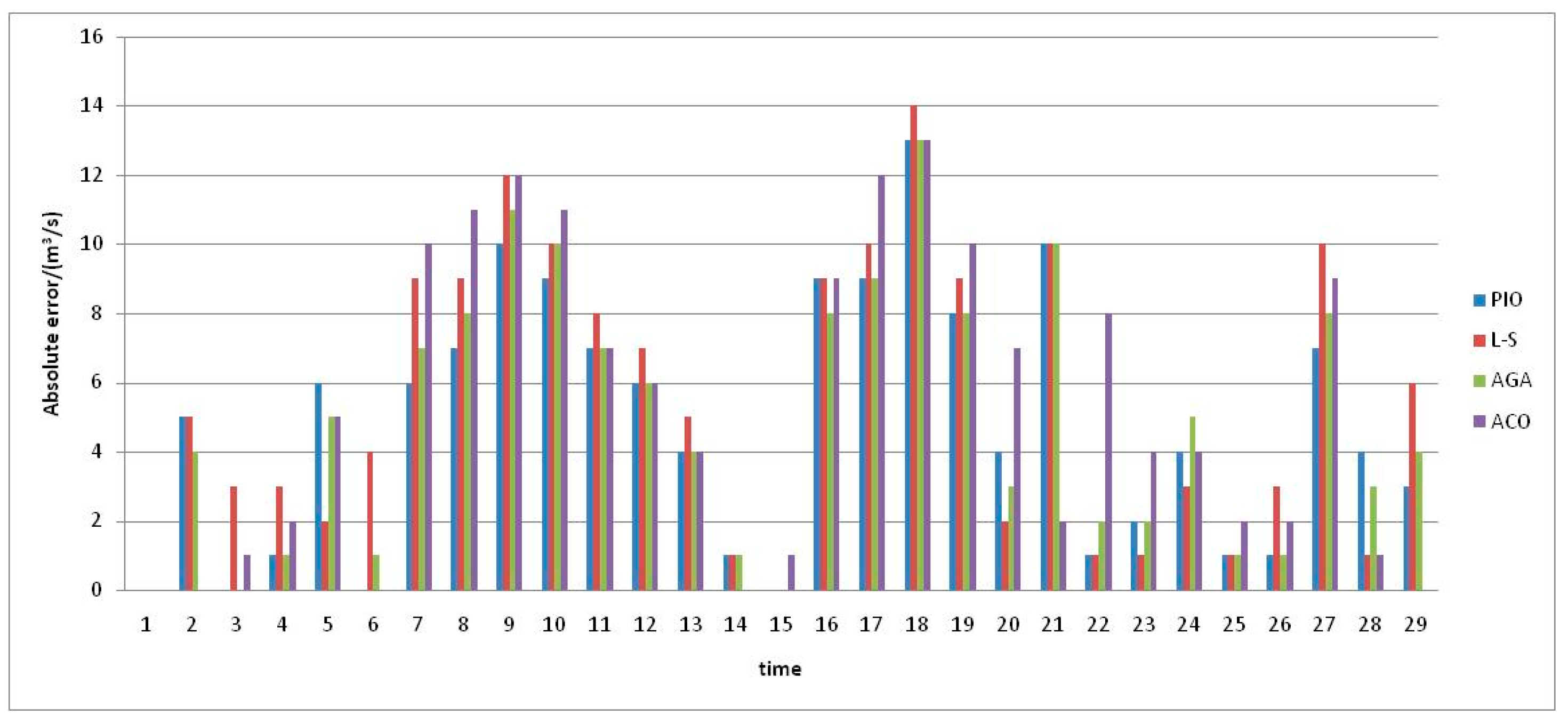
Figure 2.
Relative error results of four algorithms.

Figure 3.
Simulation results of four algorithms. Abbreviations: PIO, Pigeon-Inspired Optimization algorithm; L-S, Least-Square method; AGA, Accelerated Genetic Algorithm; ACO, Ant Colony Optimization algorithm.
Figure 3.
Simulation results of four algorithms. Abbreviations: PIO, Pigeon-Inspired Optimization algorithm; L-S, Least-Square method; AGA, Accelerated Genetic Algorithm; ACO, Ant Colony Optimization algorithm.
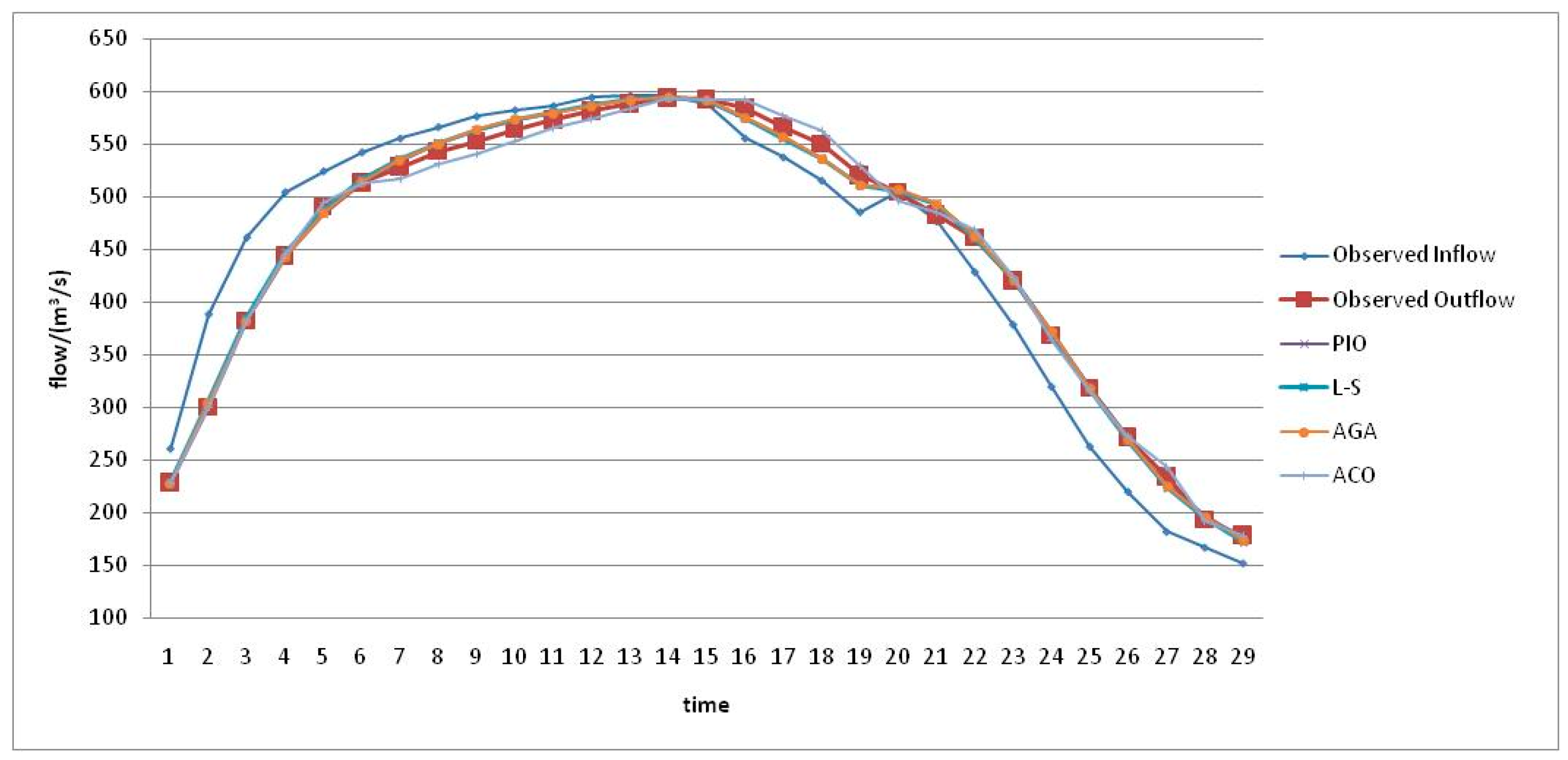
Figure 4.
Three-layer BP network.

Figure 5.
The study river channel.
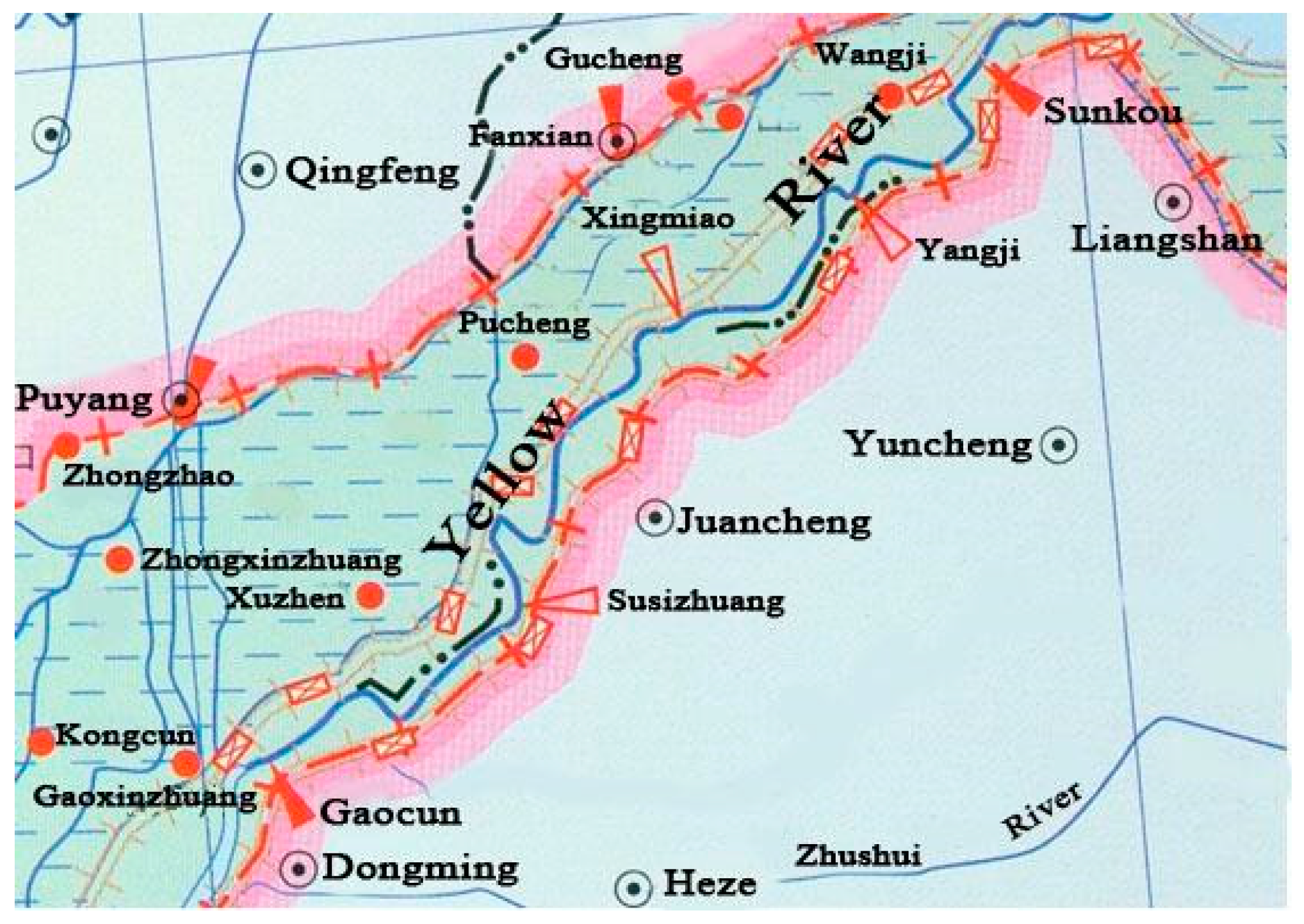
Figure 6.
Flood process diagram.
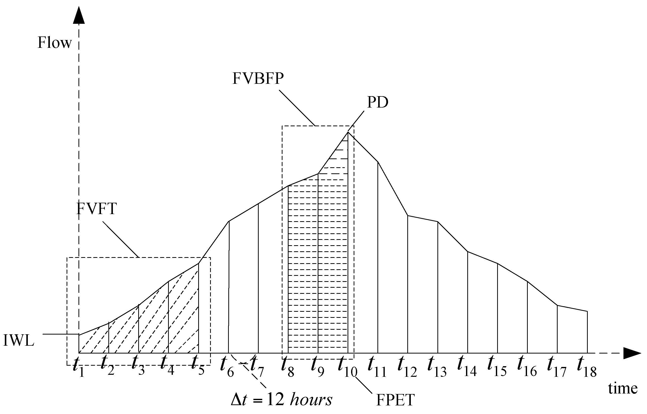
Figure 7.
Correlation between each flood characteristic attribute and Muskingum model parameters. (a) Correlation between IWL and parameter K; (b) Correlation between IWL and parameter x; (c) Correlation between PD and parameter K; (d) Correlation between PD and parameter x; (e) Correlation between FPET and parameter K; (f) Correlation between FPET and parameter x; (g) Correlation between FVFT and parameter K; (h) Correlation between FVFT and parameter x; (i) Correlation between FVBFP and parameter K; (j) Correlation between FVBFP and parameter x; (k) Correlation between ADBFP and parameter K; (l) Correlation between ADBFP and parameter x.


Figure 8.
The flow chart of the “In-Process Type” Dynamic Parameter Estimation (IP-DPE) method.
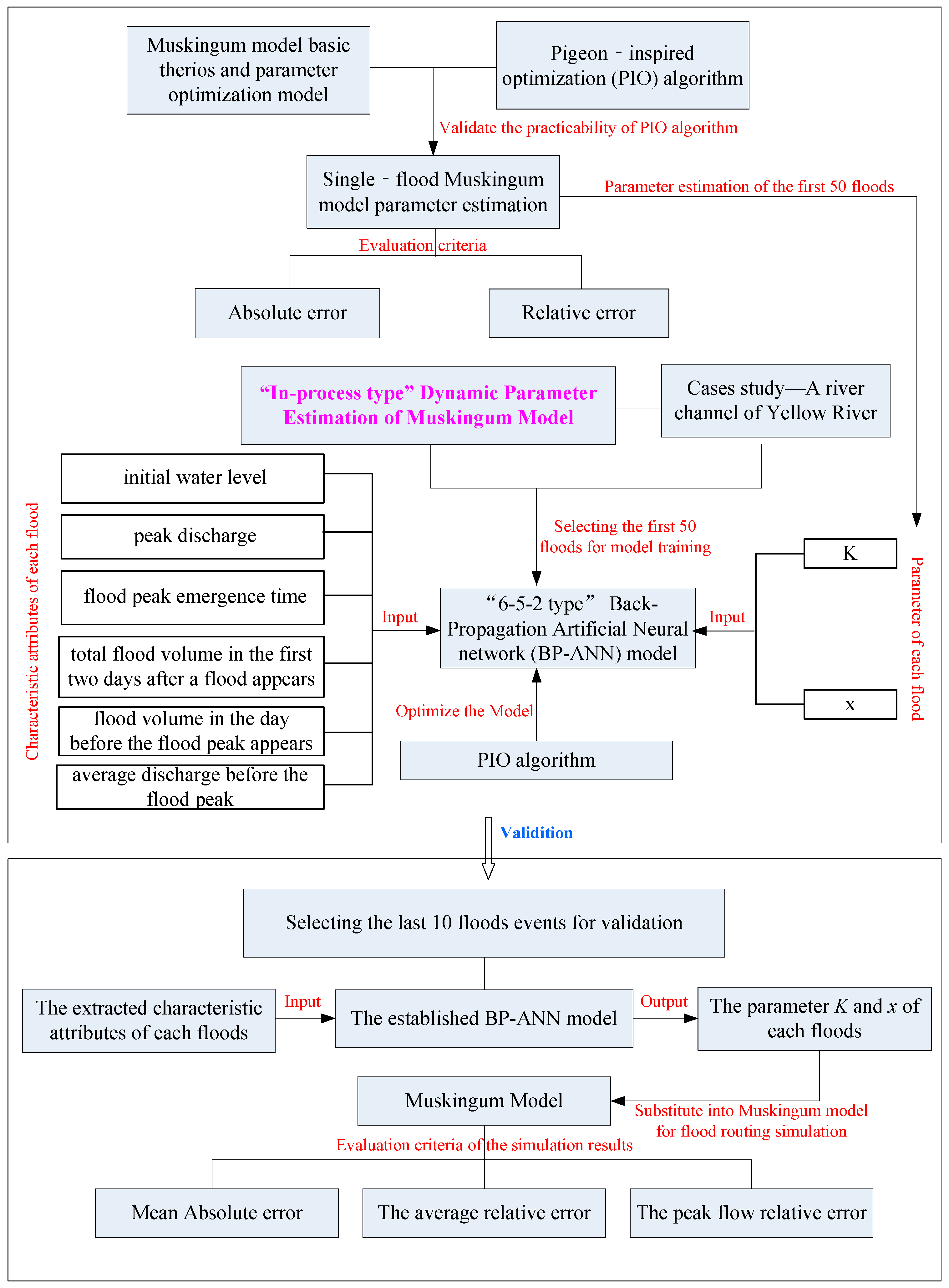
Figure 9.
Back Propagation (BP)-Neural Network structure diagram.

Figure 10.
Performance comparison between the three methods. (a) Mean absolute error comparison between three methods; (b) Average relative error comparison between three methods; (c) Peak flow relative error comparison between three methods.
Figure 10.
Performance comparison between the three methods. (a) Mean absolute error comparison between three methods; (b) Average relative error comparison between three methods; (c) Peak flow relative error comparison between three methods.
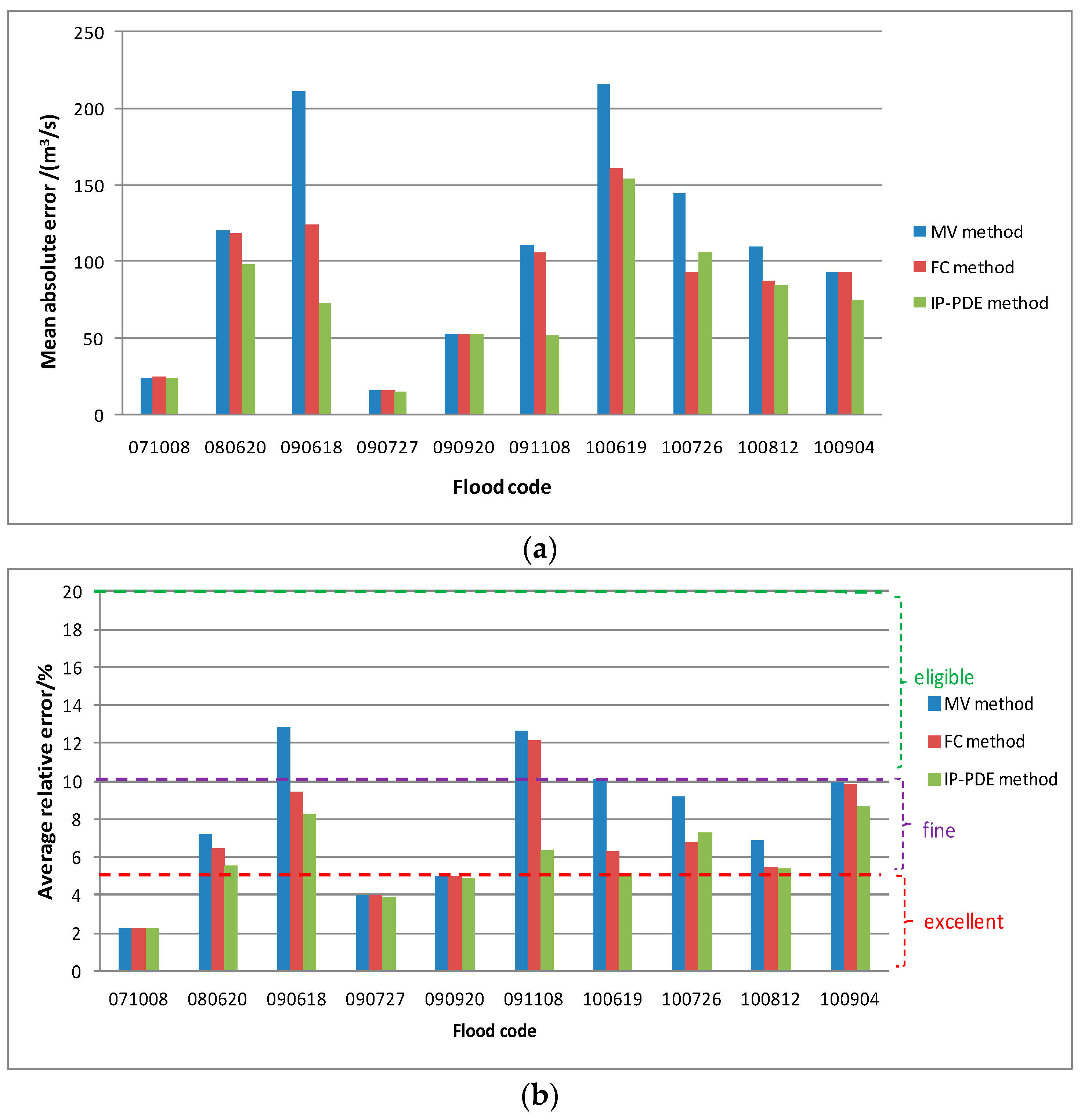

Figure 11.
Prediction results of three methods. (a) Prediction results of No. 071008 flood; (b) Prediction results of No. 080620 flood; (c) Prediction results of No. 090618 flood; (d) Prediction results of No. 090727 flood; (e) Prediction results of No. 090920 flood; (f) Prediction results of No. 091108 flood; (g) Prediction results of No. 100619 flood; (h) Prediction results of No. 100726 flood; (i) Prediction results of No. 100812 flood; (j) Prediction results of No. 100904 flood.

Table 1.
Parameter estimation results and performance comparison among four algorithms.
| PIO | L-S | AGA | ACO | |
|---|---|---|---|---|
| K | 12.536 | 11.7916 | 12.4508 | 12.7915 |
| x | −0.4189 | −0.352 | −0.356 | −0.2592 |
| Average absolute error | 4.76 | 5.63 | 5.11 | 5.23 |
| Average relative error | 1.07% | 1.29% | 1.15% | 1.18% |
Abbreviations: PIO, Pigeon-Inspired Optimization algorithm; L-S, Least-Square method; AGA, Accelerated Genetic Algorithm; ACO, Ant Colony Optimization algorithm.
Table 2.
Parameter estimation results obtained from mean value (MV) method, flow classification (FC) method, and IP-DPE method.
Table 2.
Parameter estimation results obtained from mean value (MV) method, flow classification (FC) method, and IP-DPE method.
| Flood Code | 071008 | 080620 | 090618 | 090727 | 090920 | 091108 | 100619 | 100726 | 100812 | 100904 | |
|---|---|---|---|---|---|---|---|---|---|---|---|
| MV method | 22.318 | 22.318 | 22.318 | 22.318 | 22.318 | 22.318 | 22.318 | 22.318 | 22.318 | 22.318 | |
| 0.1998 | 0.1998 | 0.1998 | 0.1998 | 0.1998 | 0.1998 | 0.1998 | 0.1998 | 0.1998 | 0.1998 | ||
| FC method | 21.851 | 10.066 | 10.866 | 31.360 | 21.409 | 23.118 | 9.005 | 14.049 | 13.690 | 20.557 | |
| 0.1998 | 0.1998 | 0.1998 | 0.1998 | 0.1998 | 0.1998 | 0.1998 | 0.1998 | 0.1998 | 0.1998 | ||
| IP-DPE method | 22.996 | 12.415 | 14.601 | 27.809 | 24.961 | 12.004 | 11.943 | 15.720 | 17.220 | 17.6342 | |
| 0.2002 | 0.1278 | 0.1170 | 0.2392 | 0.0039 | 0.3337 | 0.2203 | 0.1533 | 0.1608 | 0.0084 | ||
© 2017 by the authors. Licensee MDPI, Basel, Switzerland. This article is an open access article distributed under the terms and conditions of the Creative Commons Attribution (CC BY) license (http://creativecommons.org/licenses/by/4.0/).
Share and Cite
MDPI and ACS Style
Zhang, G.; Xie, T.; Zhang, L.; Hua, X.; Wu, C.; Chen, X.; Li, F.; Zhao, B. “In-Process Type” Dynamic Muskingum Model Parameter Estimation Method. Water 2017, 9, 849. https://doi.org/10.3390/w9110849
AMA Style
Zhang G, Xie T, Zhang L, Hua X, Wu C, Chen X, Li F, Zhao B. “In-Process Type” Dynamic Muskingum Model Parameter Estimation Method. Water. 2017; 9(11):849. https://doi.org/10.3390/w9110849
Chicago/Turabian StyleZhang, Gang, Tuo Xie, Lei Zhang, Xia Hua, Chen Wu, Xi Chen, Fangfeng Li, and Bin Zhao. 2017. "“In-Process Type” Dynamic Muskingum Model Parameter Estimation Method" Water 9, no. 11: 849. https://doi.org/10.3390/w9110849
Note that from the first issue of 2016, this journal uses article numbers instead of page numbers. See further details here.