
Long-Term Streamflow Forecasting Based on Relevance Vector Machine Model


Abstract
:1. Introduction
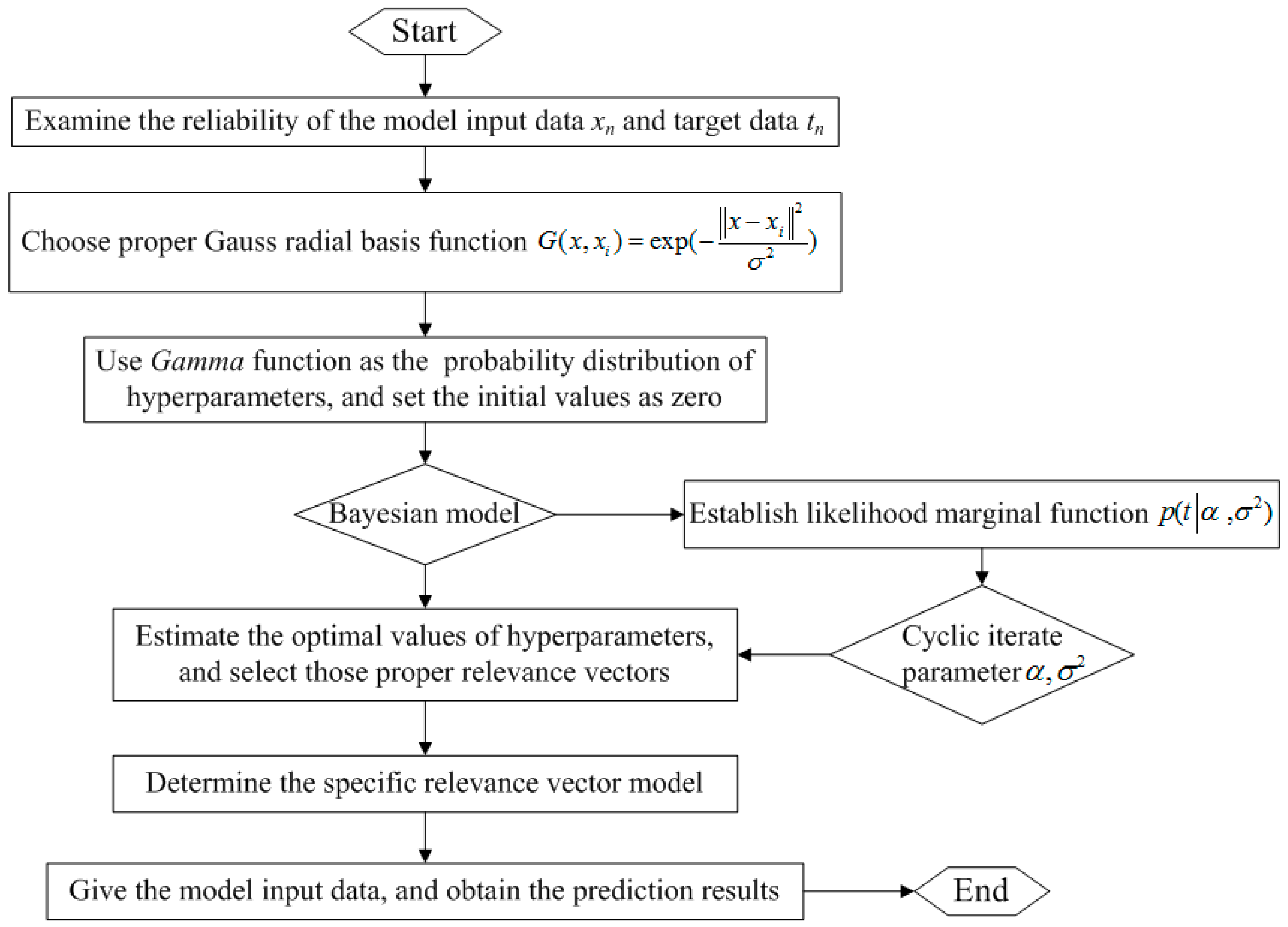
2. The RVM Model
3. Materials
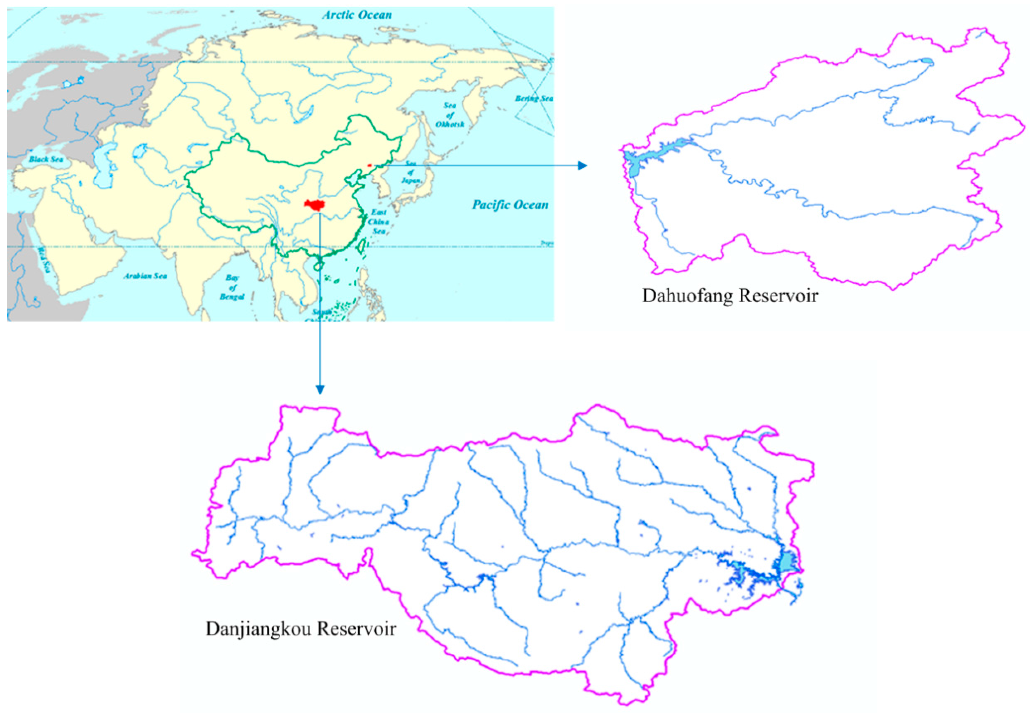
3.1. Study Area
3.2. Data Sets
4. Results and Discussion
4.1. Selection of Predictor Factors
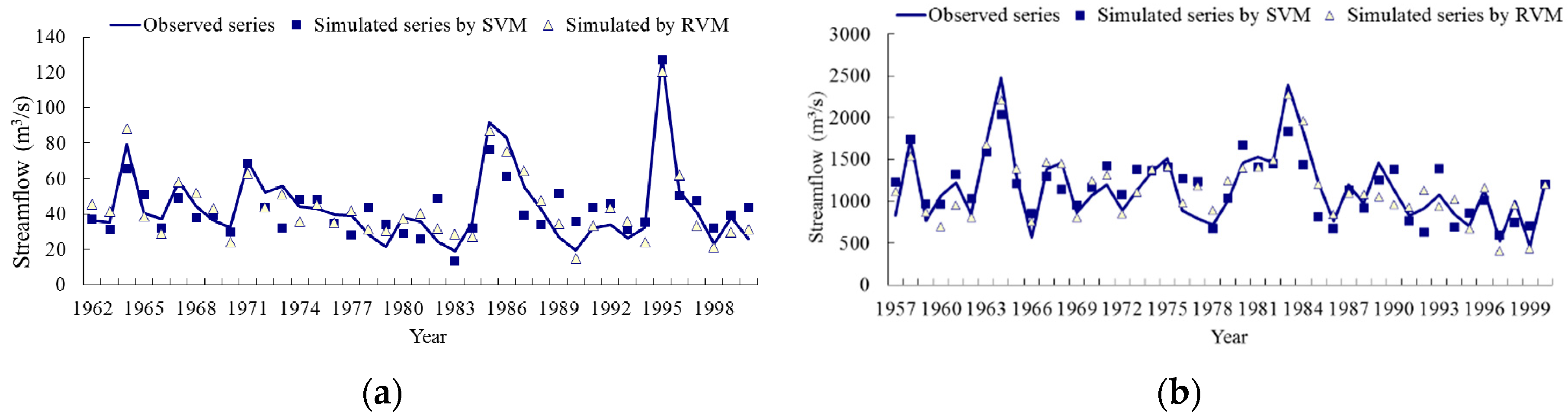
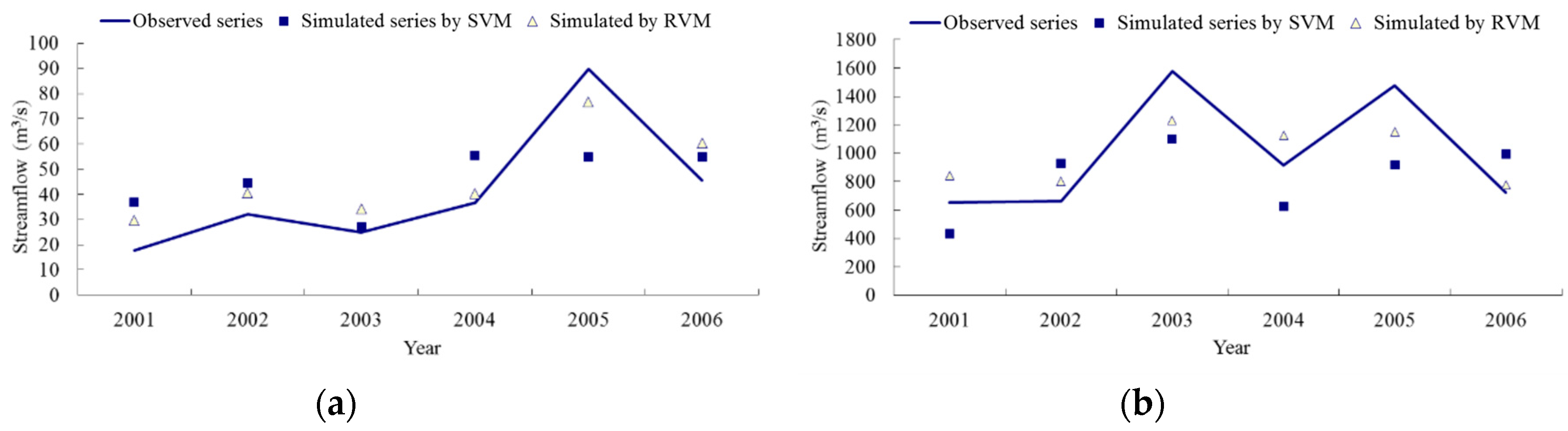
4.2. Model Performance Evaluation
4.3. Results Discussion
5. Conclusions
Acknowledgments
Author Contributions
Conflicts of Interest
References
- Sagarika, S.; Kalra, A.; Ahmad, S. Evaluating the effect of persistence on long-term trends and analyzing step changes in streamflows of the continental United States. J. Hydrol. 2014, 517, 36–53. [Google Scholar] [CrossRef]
- Shortridge, J.E.; Guikema, S.D.; Zaitchik, B.F. Machine learning methods for empirical streamflow simulation: A comparison of model accuracy, interpretability, and uncertainty in seasonal watersheds. Hydrol. Earth Syst. Sci. 2016, 20, 2611–2628. [Google Scholar] [CrossRef]
- Sang, Y.F.; Singh, V.P.; Wen, J.; Liu, C.M. Gradation of complexity and predictability of hydrological processes. J. Geophys. Res. 2015, 120, 5334–5343. [Google Scholar] [CrossRef]
- Sorooshian, S.; Dracup, J.A. Stochastic parameter estimation procedures for hydrologie rainfall-runoff models: Correlated and heteroscedastic error cases. Water Resour. Res. 1980, 16, 430–442. [Google Scholar] [CrossRef]
- Sang, Y.F. Improved wavelet modeling framework for hydrologic time series forecasting. Water Resour. Manag. 2013, 27, 2807–2821. [Google Scholar] [CrossRef]
- Zealand, C.M.; Burn, D.H.; Simonovic, S.P. Short term streamflow forecasting using artificial neural networks. J. Hydrol. 1999, 214, 32–48. [Google Scholar] [CrossRef]
- Nourani, V.; Baghanam, A.H.; Adamowski, J.; Kisi, O. Applications of hybrid wavelet–artificial intelligence models in hydrology: A review. J. Hydrol. 2014, 514, 358–377. [Google Scholar] [CrossRef]
- ASCE Task Committee. Artificial neural networks in hydrology II: Hydrologic applications. J. Hydrol. Eng. 2000, 5, 124–137. [Google Scholar]
- Gutierrez, F.; Dracup, J.A. An analysis of the feasibility of long-range streamflow forecasting for Colombia using El Nino–Southern Oscillation indicators. J. Hydrol. 2001, 246, 181–196. [Google Scholar] [CrossRef]
- Olsson, J.; Uvo, C.B.; Jinno, K.; Kawamura, A.; Nishiyama, K.; Koreeda, N. Neural networks for rainfall forecasting by atmospheric downscaling. J. Hydrol. Eng. 2004, 9, 1–12. [Google Scholar] [CrossRef]
- Guven, A.; Aytek, A.; Yuce, M.I.; Aksoy, H. Genetic programming-based empirical model for daily reference evapotranspiration estimation. Clean-Soil Air Water 2008, 36, 905–912. [Google Scholar] [CrossRef]
- Maier, H.R.; Dandy, G.C. Neural networks for the prediction and forecasting of water resources variables: A review of modeling issues and applications. Environ. Model. Softw. 2000, 15, 101–124. [Google Scholar] [CrossRef]
- Dawson, C.W.; Wilby, R.L. Hydrological modeling using artificial neural networks. Prog. Phys. Geogr. 2001, 25, 80–108. [Google Scholar] [CrossRef]
- Chau, K.W. Particle swarm optimization training algorithm for ANNs in stage prediction of Shing Mun River. J. Hydrol. 2006, 329, 363–367. [Google Scholar] [CrossRef]
- Vapnik, V.N. Statistical Learning Theory; Wiley: New York, NY, USA, 1998. [Google Scholar]
- Vapnik, V. The Nature of Statistical Learning Theory; Springer: New York, NY, USA, 1995. [Google Scholar]
- Asefa, T.; Kemblowski, M.; McKee, M.; Khalil, A. Multi-time scale stream flow predictions: The support vector machines approach. J. Hydrol. 2006, 318, 7–16. [Google Scholar] [CrossRef]
- Lu, M.; Zhang, Z.Y. Application of support vector machine in runoff forecast. China Rural Water Hydropower 2006, 2, 47–49. [Google Scholar]
- Li, Y.B.; Huang, Q.; Xu, J.X.; Zuo, W.B. Research on prediction of streamflow based on C-SVM. J. Hydroel. Eng. 2008, 27, 42–47. [Google Scholar]
- Lin, J.Y.; Cheng, C.T.; Chau, K.W. Using support vector machines for long-term discharge prediction. Hydrol. Sci. J. 2006, 51, 599–612. [Google Scholar] [CrossRef]
- Tipping, M.E. The relevance vector machine. Adv. Neural Inf. Process. Syst. 1999, 12, 652–658. [Google Scholar]
- Tipping, M.E. Sparse Bayesian learning and the relevance vector machine. J. Mach. Learn. Res. 2001, 1, 211–244. [Google Scholar]
- Tripathi, S.; Govindaraju, R.S. On selection of kernel parametes in relevance vector machines for hydrologic applications. Stoch. Environ. Res. Risk Assess. 2007, 21, 747–764. [Google Scholar] [CrossRef]
- Zaman, B.; McKee, M.; Neale, C.U. Fusion of remotely sensed data for soil moisture estimation using relevance vector and support vector machines. Int. J. Remote Sens. 2012, 33, 6516–6552. [Google Scholar] [CrossRef]
- He, F.; Li, M.; Yang, J.H.; Xu, J.W. Product quality model based on wavelet relevance vector machine. J. Univ. Sci. Technol. Beijing 2009, 31, 934–937. [Google Scholar]
- Hurrell, J.W. Decadal trends in the North Atlantic Oscillation: Regional temperatures and precipitation. Science 1995, 269, 676–679. [Google Scholar] [CrossRef] [PubMed]
- Hamlet, A.F.; Lettenmaier, D.P. Columbia River streamflow forecasting based on ENSO and PDO climate signals. J. Water Resour. Plan. Manag. 1999, 125, 333–341. [Google Scholar] [CrossRef]
- Shahab, A.; Donald, H.B.; Mohammand, K. Long-term probabilistic forecasting of streamflow using ocean-atmospheric and hydrological predictors. Water Resour. Res. 2006, 42, W03431. [Google Scholar]
- McCabe, G.J.; Betancourt, J.L.; Hidalgo, H.G. Associations of decadal to multidecadal sea-surface temperature variability with upper Colorado River flow. J. Am. Water Resour. Assoc. 2007, 43, 183–192. [Google Scholar] [CrossRef]
- Glenn, A.T.; Thomas, C.P.; Felipe, G. The relationships between pacific and Atlantic ocean sea surface temperatures and Colombian streamflow variability. J. Hydrol. 2008, 349, 268–276. [Google Scholar]
- Kalra, A.; Ahmad, S. Using oceanic-atmospheric oscillation for long lead time streamflow forecasting. Water Resour. Res. 2009, 45, W03413. [Google Scholar] [CrossRef]
- Ghosh, S.; Mujumdar, P.P. Statistical downscaling of GCM simulations to streamflow using relevance vector machine. Adv. Water Resour. 2008, 31, 132–146. [Google Scholar] [CrossRef]
- Turing, A.M. Computing machinery and intelligence. Mind 1950, 59, 433–460. [Google Scholar] [CrossRef]
- Khalil, A.F.; McKee, M.; Kemblowski, M.; Asefa, T.; Bastidas, L. Multiobjective analysis of chaotic dynamic systems with sparse learning machines. Adv. Water Resour. 2006, 29, 72–88. [Google Scholar] [CrossRef]
- Gill, M.K.; Asefa, T.; Kemblowski, M.W.; McKee, M. Soil moisture prediction using support vector machines. J. Am. Water Resour. Assoc. 2006, 42, 1033–1046. [Google Scholar] [CrossRef]
- Yu, X.; Liong, S.Y. Forecasting of hydrologic time series with ridge regression in feature space. J. Hydrol. 2007, 332, 290–302. [Google Scholar] [CrossRef]
- Gupta, H.V.; Kling, H.; Yilmaz, K.K.; Martinez, G.F. Decomposition of the mean squared error and NSE performance criteria: Implications for improving hydrological modelling. J. Hydrol. 2009, 377, 80–91. [Google Scholar] [CrossRef]
- You, H.L. Study on Method Application of Mid-long-term Runoff Forecast of Dahuofang Reservoir. Master’s Thesis, Liaoning Normal University, Dalian, China, 2010. [Google Scholar]
- Dong, Y.; Yuan, J.; Zhou, H. Research on Annual Runoff Forecasting Method for Dahuofang Reservoir. J. China Hydrol. 2008, 28, 54–56, (In Chinese with English Abstract). [Google Scholar]
- Ran, D.; Li, M.; Wu, S.; Xie, J. Research on multi-model forecasts in mid-long term runoff in Danjiangkou Reservoir. J. Hydraul. Eng. 2010, 41, 1069–1073, (In Chinese with English Abstract). [Google Scholar]
- Hu, X.; Wang, Y.; Liu, Y.; Hu, Q. Monthly runoff forecast for Danjiangkou Reservoir based on physical statistical methods. J. Hohai Univ. Nat. Sci. 2011, 39, 242–247, (In Chinese with English Abstract). [Google Scholar]
- Liu, Y.; Wang, Y.; Chen, Y. Long-term runoff forecasting for autumn flooding seasons in Danjiangkou reservoir based on analyzing the physical causes. Adv. Water Sci. 2010, 21, 41–48, (In Chinese with English Abstract). [Google Scholar]

| Order | Predictor Factor | Correlation Coefficient | Description of Factor |
|---|---|---|---|
| 1 | 500 hpa_4_218 | −0.457 | Z500 in the grid 218 in April of the last year |
| 2 | 500 hpa_3_260 | −0.397 | Z500 in the grid 260 in March of the last year |
| 3 | 500 hpa_8_164 | 0.456 | Z500 in the grid 164 in August of the last year |
| 4 | SST_9_591 | 0.490 | SSTs in the grid 591 in September of the last year |
| 5 | SST_5_409 | 0.411 | SSTs in the grid 409 in May of the last year |
| 6 | SST_3_418 | −0.408 | SSTs in the grid 418 in March of the last year |
| Order | Predictor Factor | Correlation Coefficient | Description of Factor |
|---|---|---|---|
| 1 | 500 hpa_6_193 | 0.337 | Z500 in the grid 193 in June of the last year |
| 2 | 500 hPa_4_182 | 0.471 | Z500 in the grid 182 in April of the last year |
| 3 | 500 hpa_11_126 | −0.468 | Z500 in the grid 126 in November of the last year |
| 4 | 500 hpa_7_221 | 0.451 | Z500 in the grid 221 in July of the last year |
| 5 | SST_9_187 | −0.522 | SSTs in the grid 187 in September of the last year |
| 6 | SST_7_189 | −0.395 | SSTs in the grid 189 in July of the last year |
| 7 | SST_6_412 | −0.417 | SSTs in the grid 412 in June of the last year |
| Step | Predictor Factor | Factor Number | Multiple Correlation | ||
|---|---|---|---|---|---|
| DJK | DHF | DJK | DHF | ||
| First step | Z500 | 7 | 6 | 0.90 | 0.85 |
| SST | 4 | 5 | 0.79 | 0.81 | |
| Second step | Factor set | 7 | 6 | 0.92 | 0.94 |
| Area | Data for Model Training | Data for Model Testing |
|---|---|---|
| DJK | 1962–2000 | 2001–2006 |
| DHF | 1957–2000 | 2001–2006 |
| Model | Training | Testing | ||||
|---|---|---|---|---|---|---|
| R | RMSE (m3/s) | E | R | RMSE (m3/s) | E | |
| SVM | 0.91 | 7.58 | 0.89 | 0.74 | 19.01 | 0.63 |
| RVM | 0.95 | 6.78 | 0.90 | 0.83 | 13.76 | 0.78 |
| Model | Training | Testing | ||||
|---|---|---|---|---|---|---|
| R | RMSE (m3/s) | E | R | RMSE (m3/s) | E | |
| SVM | 0.84 | 191.18 | 0.81 | 0.67 | 339.01 | 0.57 |
| RVM | 0.92 | 163.06 | 0.85 | 0.88 | 231.92 | 0.68 |
© 2016 by the authors; licensee MDPI, Basel, Switzerland. This article is an open access article distributed under the terms and conditions of the Creative Commons Attribution (CC-BY) license (http://creativecommons.org/licenses/by/4.0/).
Share and Cite
Liu, Y.; Sang, Y.-F.; Li, X.; Hu, J.; Liang, K. Long-Term Streamflow Forecasting Based on Relevance Vector Machine Model. Water 2017, 9, 9. https://doi.org/10.3390/w9010009
Liu Y, Sang Y-F, Li X, Hu J, Liang K. Long-Term Streamflow Forecasting Based on Relevance Vector Machine Model. Water. 2017; 9(1):9. https://doi.org/10.3390/w9010009
Chicago/Turabian StyleLiu, Yong, Yan-Fang Sang, Xinxin Li, Jian Hu, and Kang Liang. 2017. "Long-Term Streamflow Forecasting Based on Relevance Vector Machine Model" Water 9, no. 1: 9. https://doi.org/10.3390/w9010009
APA StyleLiu, Y., Sang, Y.-F., Li, X., Hu, J., & Liang, K. (2017). Long-Term Streamflow Forecasting Based on Relevance Vector Machine Model. Water, 9(1), 9. https://doi.org/10.3390/w9010009