Measuring Spatiotemporal Features of Land Subsidence, Groundwater Drawdown, and Compressible Layer Thickness in Beijing Plain, China

Abstract

Beijing is located on multiple alluvial-pluvial fans with thick Quaternary unconsolidated sediments. It has suffered serious groundwater drawdown and land subsidence due to groundwater exploitation. This study aimed to introduce geographical distribution measure methods into land subsidence research characterizing, geographically, land subsidence, groundwater drawdown, and compressible layer thickness. Therefore, we used gravity center analysis and standard deviational ellipse (SDE) methods in GIS to statistically analyze their concentration tendency, principle orientation, dispersion trend, and distribution differences in 1995 (1999), 2007, 2009, 2011, and 2013. Results show that they were all concentrated in Chaoyang District of Urban Beijing. The concentration trend of land subsidence was consistent with that of groundwater drawdown. The principle orientation of land subsidence was SW–NE, which was more similar with that of the static spatial distribution of the compressible layer. The dispersion tendency of land subsidence got closer to that of the compressible layer with its increasing intensity. The spatial distribution difference between land subsidence and groundwater drawdown was about 0.2, and that between land subsidence and compressible layer thickness it decreased from 0.22 to 0.07, reflecting that the spatial distribution pattern of land subsidence was increasingly close to that of the compressible layer. Results of this study are useful for assessing the distribution of land subsidence development and managing groundwater resources.

1. Introduction

Regional land subsidence is a geological process occurring in a long-run equilibrium and inter-coordination between anthropogenic activity and the hydrogeological environment [1,2]. In most areas worldwide, compressible sediments are the material basis and it unbalances the starting point of land subsidence; groundwater drawdown is an inherent drive and its spatial diversity induces an uneven development process of land subsidence [3,4,5,6,7,8,9,10,11]. Land subsidence has increased the risk of other disasters and threatened the properties of the society [12,13,14,15]. Mapping and quantifying how, and to what extent, the groundwater drawdown and compressible layer influence non-uniform land subsidence based on multiple time-series displacement and hydrogeological data are of concern to many scholars [16,17,18,19,20].

Land subsidence in Beijing Plain is mainly triggered by over-exploitation of groundwater, and its magnitude and extent is affected by heterogeneity of compressible layers [21]. Integrated subsidence-monitoring programs with multiple surveying methods were designed to clarify both hydrological and mechanical processes of land subsidence [22]. The persistent scatterer interferometry (PSI) technique was adopted to quantify the dynamic evolution of land subsidence in the Beijing north plain, and to determine the spatial relationship with its triggering factors [23]. The small baseline interferometric synthetic aperture radar (InSAR) [24] technique was employed to investigate the relationship between land subsidence and groundwater level, active faults, cumulated soft soil thickness, different aquifer types, and the distance to pumping wells [10]. These studies proved that the spatial extent and magnitude of land subsidence in Beijing Plain has both spatial variability and inheritance. They paid much attention to adopting a GIS spatial overlay or visualization, focusing on its spatial extent, magnitude, and spatial correlation with groundwater drawdown, and the geological structural control at the macro scale, but it has been rarely reported that Geographic Distribution Measuring methods [25] were used to measure the distribution of subsidence-related temporal-spatial datasets that allows one to quantify their concentration tendency, development orientation, dispersion trend, and distribution differences and track their changes over time.

Gravity center analysis is an aggregated statistical method in geographical space. The gravity center dynamic could reveal the spatial concentration of geographical phenomena. It was widely used to assess spatial distribution evolvement in many fields, like population, economics, and employment [26,27]. The deviation direction indicates the adjustment of high intensity, and the deviation distance indicates the degree of equilibrium or adjustment magnitude [26]. The standard deviational ellipse (SDE) was first proposed by Lefever [28] to reveal characteristics of geospatial distribution [29,30,31,32]. It has been widely used in urban science [33,34], ecology [35,36], geology [37,38], and infectious disease distribution [39]. Mapping distributional trends for a set of violent events might identify a relationship to particular features, like ethnicity, terrain, land cover, targets, and separatist tradition [40]; comparing the size, shape, and overlap of ellipses for population, gross domestic product, and topography might provide insights regarding economic spatial variation [41]. Plotting ellipses across time series for PM_2.5 (aerosol particles smaller than 2.5 μm in diameter that are suspended in the air) concentrations might characterize the overall spatial dynamic process [42].

Therefore, this study adopted the two Geographic Distribution Measuring methods to calculate the gravity center and SDE of land subsidence, groundwater drawdown, and compressible layer thickness. Then, by comparing their parameters across time series, the understanding of their spatial distribution evolution and spatial correlation was improved. The main objective of this current study is three-fold: to introduce geographic distribution measuring methods into land subsidence research based on GIS spatial technology; to quantify the spatiotemporal distribution of land subsidence and its influencing factors in the development center, principle orientation, and dispersion, tracking their spatial distribution characteristics; and to distinguish their spatial distribution differences.

2. Materials and Methods

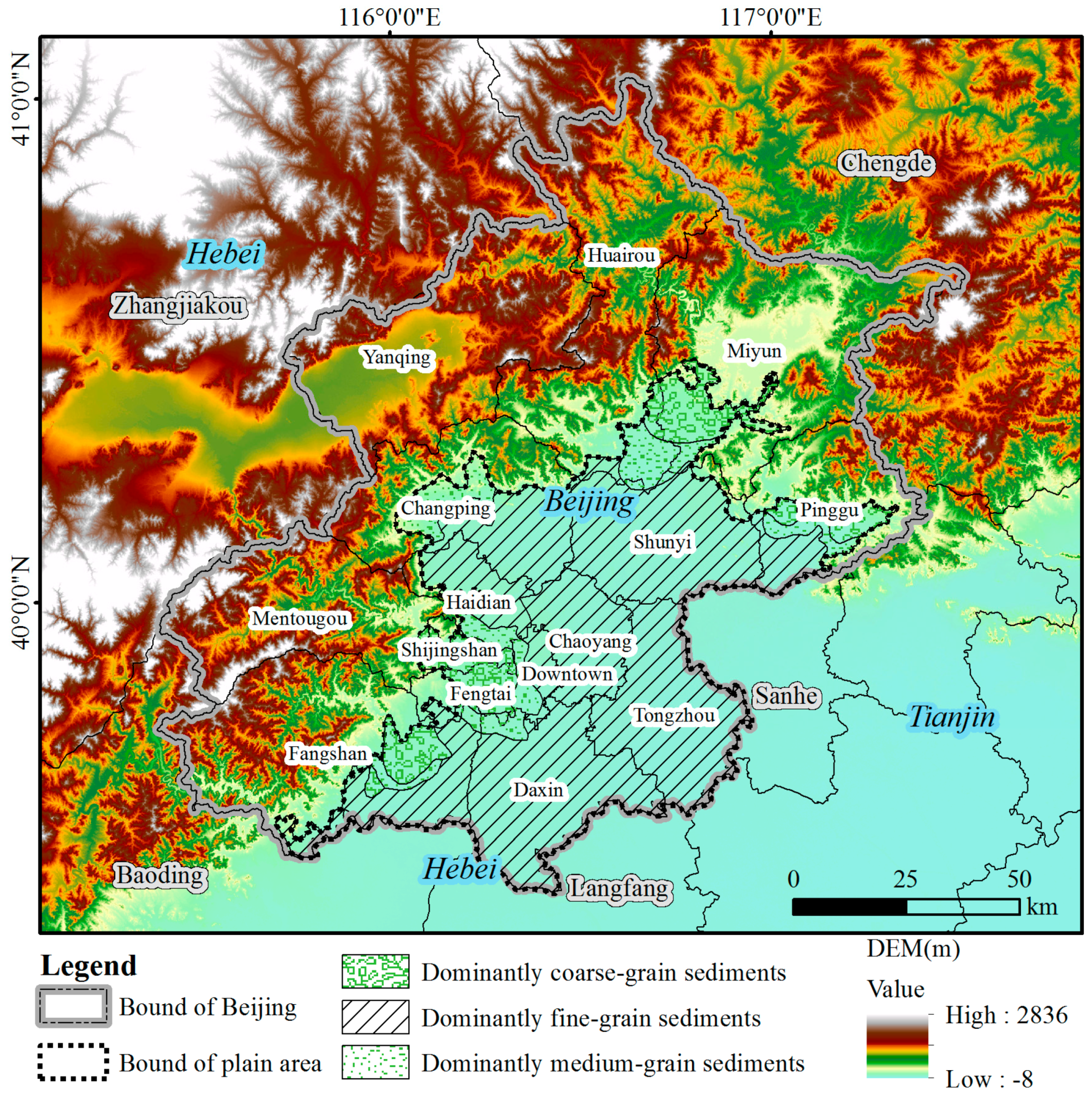
2.1. Study Area

The Beijing Plain (excluding Yanqing region) is located in the southeast part of Beijing, covering a total area of 6390 km², about 38% of Beijing (Figure 1). It lies in the alluvial-pluvial plain fan which was built up by the river deposits primarily from five rivers, including Yongding, Chaobai, Wenyu, Dashi and Jiyun Rivers. Urban districts include downtown, Chaoyang, Haidian, Shijingshan, and Fengtai. The average annual temperature is about 10–15 °C, and precipitation is 601.7 mm, which belongs to the temperate continental monsoon climate. Land subsidence is one of the critical threats to the sustainable development of Beijing city.

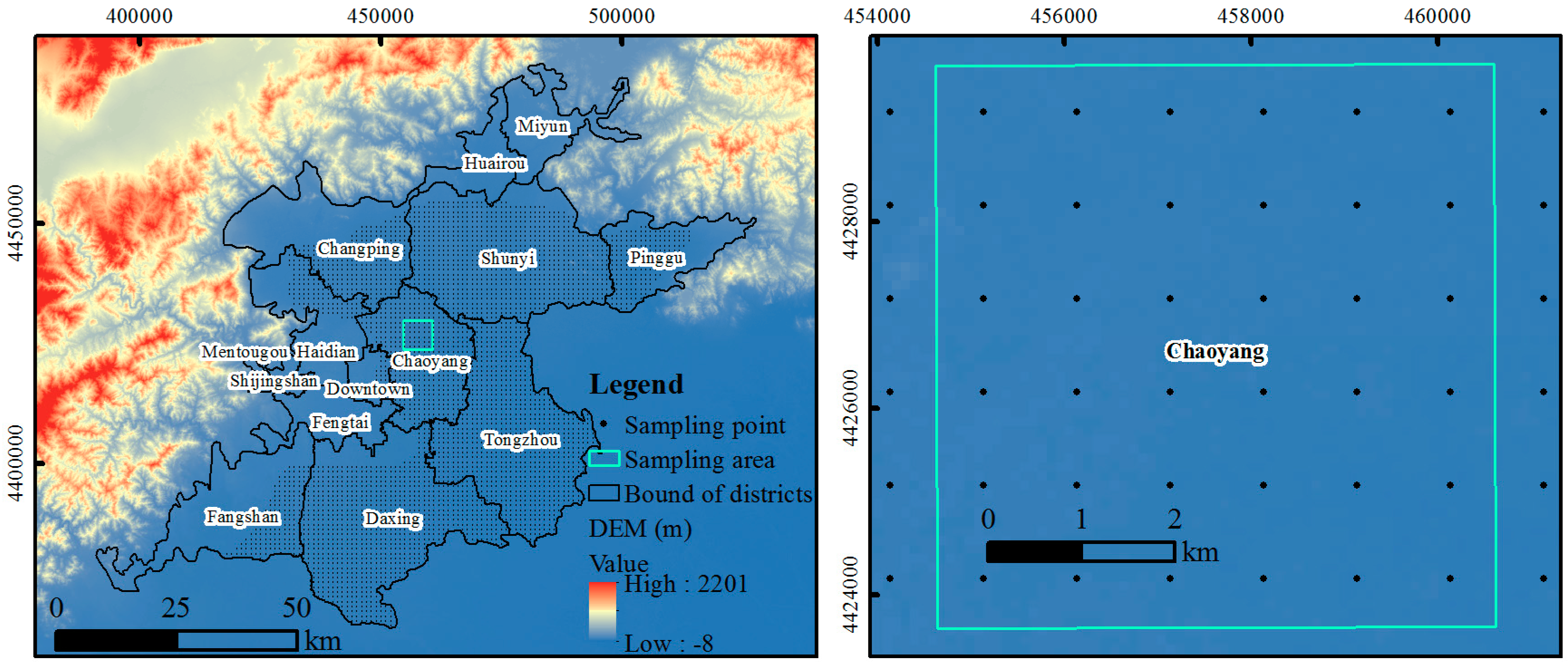
2.2. Available Datasets

Cumulative subsidence contours (the starting time was 1955) in 1999, 2007, 2009, 2011, and 2013 were derived from the Beijing land subsidence monitoring network (Figure 2). The total mean square error of leveling per kilometer and the mean square error of point locations conform to the national norms of primary leveling and second-class leveling (GB12897-91) [43]. This level monitoring network includes 278 monitoring points that provide elevation observation, and monitoring frequency is once a year. By comparing current observations and previous ones, land subsidence of the observation points were identified and then a cumulative land subsidence contour map was plotted. By 2013, the area where cumulative subsidence was greater than 100 mm reached 4942 km². A, B, C, D, E, and F referred to typical funnel zones and their maximum values are shown in

Table 1. Maximum values of the subsidence funnel zone (mm).

	Subsidence Funnel Zone	1999	2005	2007	2009	2011	2013
A	Balizhuang-Dajiaoting in Chaoyang	700	750	750	800	1050	1300
B	Laiguangying in Chaoyang	500	650	800	950	1000	1400
C	Shahe-Baxianzhaung in Changpiing	650	1050	1100	1150	1200	1400
D	Lixian-Yufa in Daxing	650	800	850	950	1050	1200
E	Pinggezhuang in Shunyi	250	400
F	Yang town in Shunyi		150	200	250	300	400

. The sedimentary time, genetic type, lithology, structure, thickness, and physical and mechanical properties of Quaternary strata are complicated and affect the occurrence and development of land subsidence in Beijing Plain. The thickness map (Figure 3) was derived after grouping silty clay, clay, silt, and other compressible sediments into a compressible layer [44]. Groundwater level observations in 1965, 1995, 2007, 2009, 2011, and 2013 were collected to delineate the changes of the groundwater seepage field (Figure 4). They are retrieved from official reports published by the Beijing Water Authority and the data are accurate and reliable [45]. Compared with that in 1965 in the natural state, fluctuating with terrain changes, the groundwater level in 2013 dropped significantly. Typical funnels of greater than −15 m have formed especially in the regions where Changping, Shunyi, and Chaoyang join together.

Considering the smallest distance between two original isolines is larger than about 100 m in the area with the most serious land subsidence, the contour map was interpolated as a raster map with a 100 m resolution to keep the overall trend reflected by the map. Spatial sampling was performed to derive 3872 samples at an interval of 1000 m according to the completeness and coverage of data. The discrete point set could be used for spatial-temporal statistics calculation and assessment (Figure 5). Each sampling point can be regarded as a case with geographic coordinates (x_i, y_i) (i = 1, 2, …, n). The weight of geographic phenomena corresponding to each case was w_i. The groundwater drawdown was the groundwater level in 1965 minus that of the target year, because the groundwater seepage field in 1965 can be approximately regarded as that of 1955.

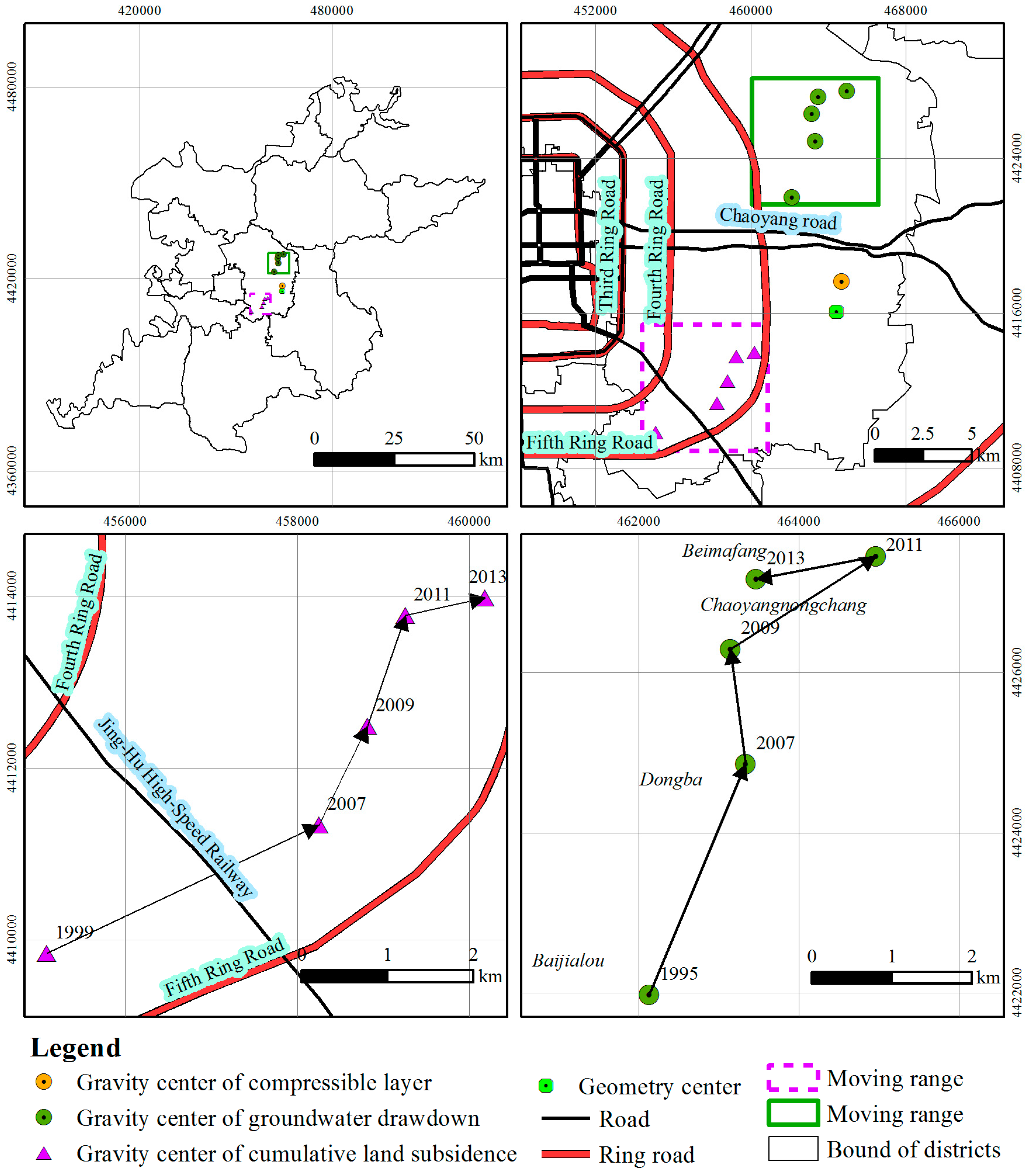
2.3. Gravity Center Analysis

The position of the gravity center was calculated using a combination of geographical coordinates and geographic space phenomena. It was extended from the concept of the spatial mean [46] and expressed as follows [26,27]:

$$\{\begin{array}{c}\overline{x}={\displaystyle \sum _{i=1}^n{w}_i{x}_i/{\displaystyle \sum _{i=1}^n{w}_i}}\\ \overline{y}={\displaystyle \sum _{i=1}^n{w}_i{y}_i/{\displaystyle \sum _{i=1}^n{w}_i}}\end{array},$$

(1)

where $\overline{x}$ and $\overline{y}$ represent the longitude and latitude coordinates (respectively) of gravity center.

According to Equation (1), if sampling points are evenly distributed and geographic space phenomena are homogeneous, the gravity center is equivalent to the regional geometric center. When the gravity center of the geographic space phenomena shows a significant offset from its regional geometric center, it indicates its disproportionate spatial distribution or gravity center deviation. In our study, gravity center motion is caused by uneven development of land subsidence. Based on tracking the gravity center derived from long-term monitoring data, its direction and distance of deviation can reflect the adjustment direction and magnitude of land subsidence. Similarly, the method can also be used to measure the influential factors of land subsidence in spatial variation features and, by comparing their movement, the influencing mode will be clarified from the macroscopic prospective.

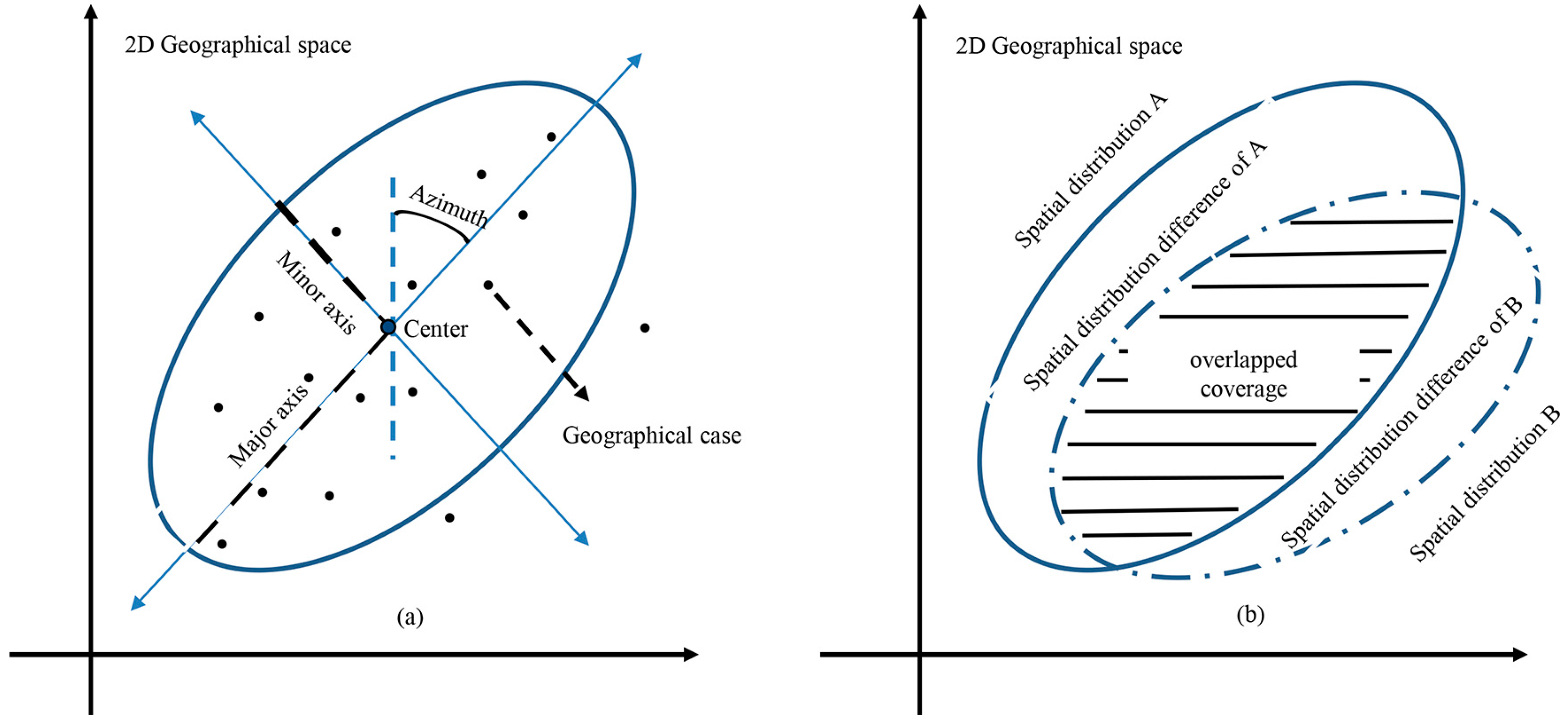
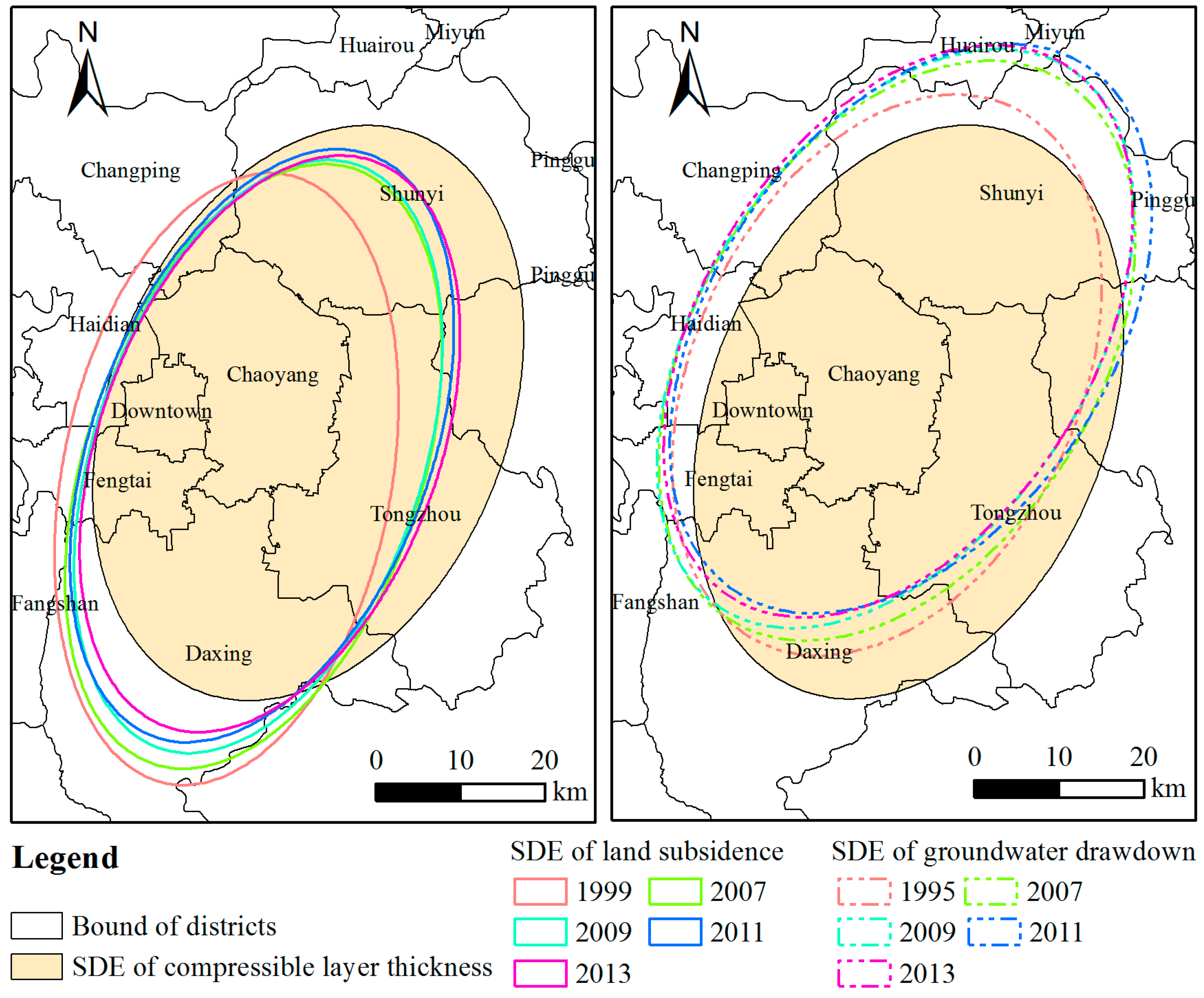
2.4. Standard Deviational Ellipse Analysis

SDE [28] is based on the average center of a set of discrete points, and the calculation of the standard distance of other points away from the average center separately in the x and y directions. These two measures define the axes of an ellipse encompassing the distribution of features. This calculated ellipse covers the spatial center, extent, orientation, shape, and other aspects, with the specific indicators are represented by the average center, the SDE, major and minor axes, and azimuth (Figure 6a). When the SDE was weighted by an attribute value associated with the features, it was termed as a weighted SDE, and the weighted average center can be expressed as shown in Equation (1). The other main parameters and corresponding equations of the weighted SDE are shown in

Table 2. The main parameters and corresponding equations of weighted standard deviational ellipse (SDE).

Parameter	Equation
Azimuth angle	$tan \theta =\frac{\left({\displaystyle \sum _{i=1}^n{w}_i^2{\stackrel{⌢}{x}}_i^2}-{\displaystyle \sum _{i=1}^n{w}_i^2{\stackrel{⌢}{y}}_i^2}\right)+\sqrt{{\left({\displaystyle \sum _{i=1}^n{w}_i^2{\stackrel{⌢}{x}}_i^2}-{\displaystyle \sum _{i=1}^n{w}_i^2{\stackrel{⌢}{y}}_i^2}\right)}^2+4{\left({\displaystyle \sum _{i=1}^n{w}_i^2{\stackrel{⌢}{x}}_i{\stackrel{⌢}{y}}_i}\right)}^2}}{2{\displaystyle \sum _{i=1}^n{w}_i^2{\stackrel{⌢}{x}}_i{\stackrel{⌢}{y}}_i}}$
Standard deviation	${\sigma }_x=\sqrt{\frac{{\displaystyle \sum _{i=1}^n{\left(w_i{\stackrel{⌢}{x}}_{i}cos\theta -w_i{\stackrel{⌢}{y}}_{i}sin\theta \right)}^2}}{{\displaystyle \sum _{i=1}^n{w}_i^2}}}$	${\sigma }_y=\sqrt{\frac{{\displaystyle \sum _{i=1}^n{\left(w_i{\stackrel{⌢}{x}}_{i}sin\theta -w_i{\stackrel{⌢}{y}}_{i}cos\theta \right)}^2}}{{\displaystyle \sum _{i=1}^n{w}_i^2}}}$

. θ refers to the azimuth of the ellipse; σ refers to the standard deviation. ${\stackrel{⌢}{x}}_i$ and ${\stackrel{⌢}{y}}_i$ refers to the distance of the point i away from the average center separately in the x and y directions. The SDE represents elements in the main distribution area; the major axis and minor axis correspond to the dispersion degree of geographical features in the principle and secondary direction; the azimuth reflects the main trend directions, allowing one to see if the distribution of features is elongated and, hence, has a particular orientation. The orientation is the rotation of the long axis measured clockwise from north. While one can get a sense of the orientation by drawing the features on a map, calculating the SDE makes the trend clear [42].

By comparing SDEs across time series, it is possible to characterize the overall spatial dynamic process. The dynamic of the center reveals the overall evolutionary track of elements; changes in the dimensions of the major and minor axes of an ellipse indicates an expansion or contraction of a specific spatial direction; and changes in the azimuth reflect the changes of overall elements in a particular spatial direction. In addition, the spatial differentiation coefficient was defined [41] to characterize the differentiation degree between different geospatial phenomena (Figure 6b). For instance, I_B/A referring to the spatial differentiation coefficient of geospatial phenomena of B relative to A can be expressed as:

$$I_{B/A}=\frac{C_B\left(A\cap B\right)}{B},$$

(2)

3. Results

3.1. Gravity Center Evolution Analysis

3.1.1. Gravity Center of Land Subsidence

The gravity centers of land subsidence in Beijing Plain were located to the southeast of downtown in Chaoyang District from 1999 to 2013, and they were distributed between Fourth Ring Road and Fifth Ring Road (Figure 7). From Figure 2 and Table 1, we can see that (1) three main subsidence funnels were located within or nearby Chaoyang district; and (2) the Lixian-Yufa subsidence area was located at the southernmost tip and far away from the urban district. This indicates that the spatial pattern of land subsidence determines the gravity center location.

Table 3. Gravity center (the relative distance and direction are relative to the geometric center).

	Year	x	y	Distance (m)	Direction	Rate (m/Year)	Relative Distance (m)	Relative Direction
Cumulative land subsidence	1999	455,082.73	4,409,843.56				11,221.13	South by West 33.70°
	2007	458,249.82	4,411,339.05	3502.42	North by East 64.72°	437.80	7773.48	South by West 37.49°
	2009	458,814.36	4,412,488.92	1280.98	North by East 26.15°	640.49	6650.08	South by West 32.58°
	2011	459,259.27	4,413,771.85	1357.88	North by East 19.13°	678.94	5647.37	South by West 24.01°
	2013	460,186.49	4,413,978.36	949.93	North by East 77.44°	474.97	4720.14	South by West 26.30°
Groundwater drawdown	1995	462,135.93	4,421,975.89				6331.38	North by West 21.13°
	2007	463,338.85	4,424,859.60	3124.55	North by East 22.64°	260.38	8855.55	North by West 7°
	2009	463,147.88	4,426,294.86	1447.90	North by West 7.58°	723.95	10,303.39	North by West 7.08°
	2011	464,963.60	4,427,455.10	2154.77	North by East 57.42°	1077.38	11,398.14	North by East 2.74°
	2013	463,472.92	4,427,165.65	1518.53	South by West 10.99°	759.27	11,135.78	North by West 4.87°
Compressible layer thickness		464,698.89	4,417,620.02				1575.25	North by East 10.28°
Geometry center		464,417.87	4,416,070.03

shows that the gravity center of land subsidence experienced an accelerating- stabilizing-reducing move north by east yearly, approaching the geometric center. From 2007 to 2011, the gravity center moved to the northeast at a higher speed. After 2011, its speed slowed and the direction was more biased to the geometric center. Figure 2 shows that the first five typical subsidence funnels have taken shape and the whole extent has kept stable since 1999; the two funnels in Chaoyang mainly moved eastwards; the Lixian-Yufa subsidence area expanded north. From 2003 to 2010, the new Yang town funnel formed, owing to continuous overexploitation and it developed to the northeast compared with the old funnel [23]; the maximum of funnels in Chaoyang district reached 110 mm/year, while that in Changping district was moderate [10]. Generally speaking, the movement of the gravity center depended on the development trend of land subsidence. It produced a small shift from southwest to northeast, presenting a total stability of spatial distribution.

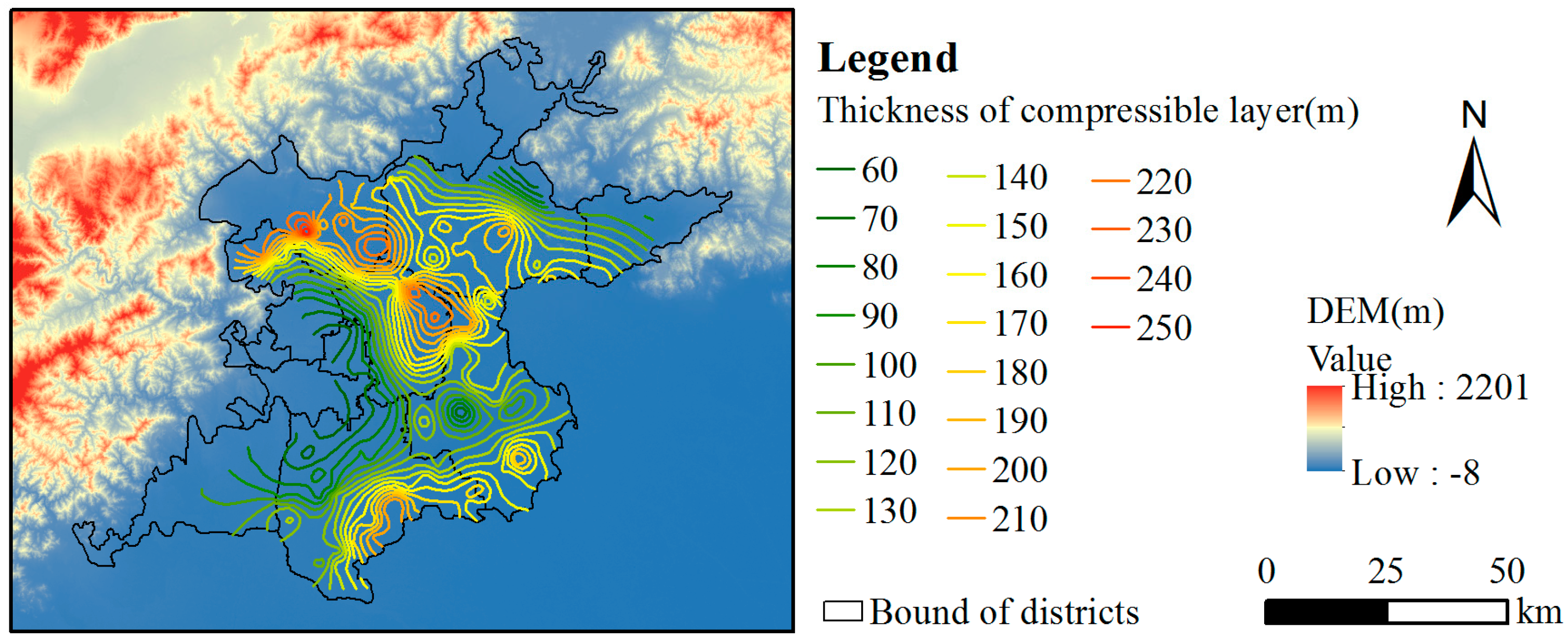
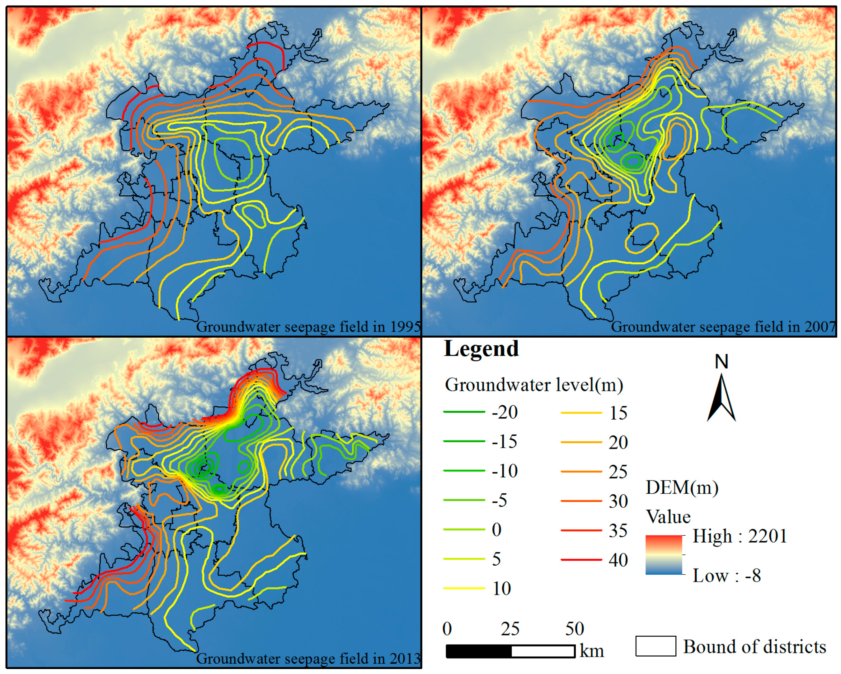
3.1.2. Gravity Center of Groundwater Drawdown and Compressible Layer Thickness

The gravity centers of groundwater drawdown in Beijing Plain were also located in Chaoyang District, to the northeast of downtown from 1999 to 2013, and they were to the northeast of the intersection of Chaoyang Road and Fifth Ring Road (Figure 7). This is because its main funnels were always distributed in the northeast of Chaoyang District and its extent fluctuated, but basically covered this area (Figure 4). The gravity center movement also experienced an accelerating-steady-reducing process (Figure 7 and Table 3). It moved north by east from Baijialou in 1995 to Dongba in 2007. From 2007 to 2009, its movement speed increased more than three times and the direction was biased to the west. From 2009 to 2011, its direction returned to north by west. After that, it moved south by west to Beimafang and the movement rate was slowed down.

The groundwater variation determined the gravity center movement dynamic. With the continuous overexploitation of groundwater through many years, the groundwater depression expanded in the northeast part of Beijing Plain, resulting in the gravity center moving northward. According to the statistics of the Beijing Water Authority, groundwater storage increased only in 2012 and it decreased more or less in other years (Figure 8). In 2012, the average annual precipitation of the whole city was 708 mm, 28% more than that in 2011, and 21% more than the average for previous years. Considering that precipitation is the main recharge for groundwater in Beijing Plain, a plentiful supply of groundwater in 2012 led to a rebound of 0.67 m of the average groundwater level compared with 2011. The estimated groundwater storage increased by 3.4 × 10⁹ m³ and the dramatic groundwater decline trend was alleviated.

The gravity center of the compressible layer was located in east-central Chaoyang District, close to the geometric center (Figure 7). It was located on the northeast part of the Yongding alluvial-pluvial fan-fringe area, and also close to the of Chaobai fan-fringe area with mass compressible deposits, reflecting the spatial concentration of the compressible layer (Figure 3).

3.1.3. Coupling Analysis of the Gravity Center

The gravity center dynamic demonstrated the adjusting direction and intensity of land subsidence, groundwater drawdown, and compressible layer thickness. The length of the connecting line (

Table 4. Coupling parameters of the gravity center. Note the cumulative land subsidence from 1955 to 1999 and the groundwater drawdown from 1965 to 1995 were compared because of the missing of same period. The same process was also seen in below.

Year	1995 (1999)	2007	2009	2011	2013
Land subsidence vs. groundwater drawdown (m)	14,033.57	14,446.58	14,470.08	14,824.67	13,590.63
Land subsidence vs. compressible layer thickness (m)	12,367.04	9002.28	7807.42	6663.16	5798.57

) between them can reflect their relative adjusting trend. For land subsidence and groundwater drawdown, it increased in 2011, and then decreased. For land subsidence and compressible layer thickness, it decreased in 2013. This suggested that the concentration trend of land subsidence showed a larger difference with that of groundwater drawdown yearly until 2011, but it decreased sharply from 2011 to 2013. In light of the largely increasing groundwater recharge from precipitation in 2012, the decrease of groundwater drawdown slowed subsidence development. The concentration trend of land subsidence illustrated a smaller difference with that of the compressible layer thickness yearly, tending to be similar with that of the latter. This reflected their increasing spatial agreement.

Groundwater drawdown is a dynamic factor, which triggers land subsidence. The compressible layer is a static factor, which provides a potential medium for land subsidence. Under the context of urbanization, the high intensity of groundwater exploitation gradually moved to the upper part of the alluvial-pluvial plain fan, with more groundwater sources. Although the compressible sediments reduced relatively, it still exists and breeds severe land subsidence [23]. Thus, the synchronized behavior of land subsidence and groundwater drawdown made the length of the connecting line change slightly. With the development of land subsidence and the groundwater drawdown, partially- or fully-developed subsidence existed in the static compressible layer. Owing to the positive correlation between the magnitude of land subsidence and the thickness of the compressible layer, the more developed the land subsidence, the thicker the compressible layer. The length of the corresponding connecting line is, therefore, getting shorter. We can make an assumption that when the potential provided by the compressible layer is exhausted, the development of land subsidence will hit a plateau. This still needs continuous observation and further study.

3.2. Development Orientation Comparison Analysis

The change tendency of the principle orientation can be analyzed by the azimuth of the ellipse’s major axis. From 1999 to 2013, the spatial direction of land subsidence development was SW–NE, showing a generally increasing trend north by east (Figure 9). From 1999 to 2007, the azimuth was increased with an average annual offset angle of 0.94°; from 2007 to 2009, the azimuth was enabled to maintain at about 18.70°; from 2011 to 2013, the azimuth was enabled to maintain at about 20.50° (

Table 5. SDE parameters of land subsidence, groundwater drawdown, and compressible layer thickness.

SDE Parameters	Year	Short Axis (m)	Long Axis (m)	Rotation Angle (°)	Long Axis/Short Axis	Area (km2)
Cumulative land subsidence	1999	19,346.19	36,550.69	11.19	1.89	2221.28
	2007	19,789.50	36,998.78	18.72	1.87	2300.04
	2009	19,348.78	36,293.81	18.67	1.88	2205.97
	2011	19,875.39	36,567.86	20.58	1.84	2283.12
	2013	19,904.22	35,492.24	20.51	1.78	2219.19
Groundwater drawdown	1995	22,751.85	34,974.82	24.96	1.54	2499.73
	2007	23,714.93	37,426.64	31.52	1.58	2788.20
	2009	22,851.41	37,940.96	32.96	1.66	2723.58
	2011	23,416.54	37,325.74	33.87	1.59	2745.69
	2013	23,009.21	37,143.34	31.94	1.61	2684.74
Compressible layer thickness		23,473.52	35,233.51	21.62	1.50	2598.10

). For groundwater drawdown weighted SDE, the azimuth was 24.96° north by east in 1995; it increased to 31.52° in 2007, at the ratio of 0.55°/year to the east. From 2007 to 2011, the azimuth increased and the rate was 0.58°/year, which was the same with that in the previous period; from 2011 to 2013, there was a sharp counter-clockwise shift (Table 5).

By comparison, the azimuth of the cumulative subsidence weighted SDE changed with that of groundwater drawdown, but was confined by that of the compressible layer thickness. The azimuth of the cumulative subsidence weighted SDE was at least 11° smaller than that of groundwater drawdown in the same year. They all had a growing tendency to north by east with some fluctuations and a peak in 20.58°. The principle direction of the cumulative subsidence weighted SDE rotated north by east, and the largest in 2009 was close to, but less than, that of the compressible layer thickness weighted SDE. This suggested that land subsidence was driven by the groundwater drawdown, but confined by the compressible layer in extent and magnitude because the thicker compressible layer is the material for land subsidence.

3.3. Dispersion Tendency Comparison Analysis

The major axis and its ratio with the minor axis characterized the spatial dispersion tendency. From 1999 to 2007, the major axis length of the land subsidence weighted SDE increased at a rate of 56 m/year; from 2007 to 2009, it decreased by 704.97 m; and from 2011 to 2013, there was another stronger spatial contraction. The corresponding ratio was reduced from 1.89 in 1999 to 1.78 in 2013 (Table 5). The spatial contraction of the ellipse suggested the central region experienced more serious land subsidence than that in the external ellipse most of the time.

From 1995 to 2007, the major axis of the groundwater drawdown weighted SDE increased at the annual rate 204.32 m/year; since 2007, its length was generally kept above 37,000 m, and there was a peak in 2009 (Table 5). Since precipitation is the main recharge of groundwater, the groundwater drawdown varied with its fluctuation and there was an apparent trough in the total precipitation and corresponding total groundwater storage especially in 2009 (Figure 8). This suggested that the length of the major axis can be regarded as an important index to measure the groundwater drawdown.

By comparison, the major axis length of the land subsidence weighted SDE decreased and approached that of the compressible layer thickness. In addition, from 1999 to 2013, the ratio between the length of the major axis and the minor axis of the land subsidence weighted SDE was reduced more closely to that of the compressible layer thickness. This suggested that the land subsidence distribution pattern got closer to that of the compressible layer with the increase of its development intensity.

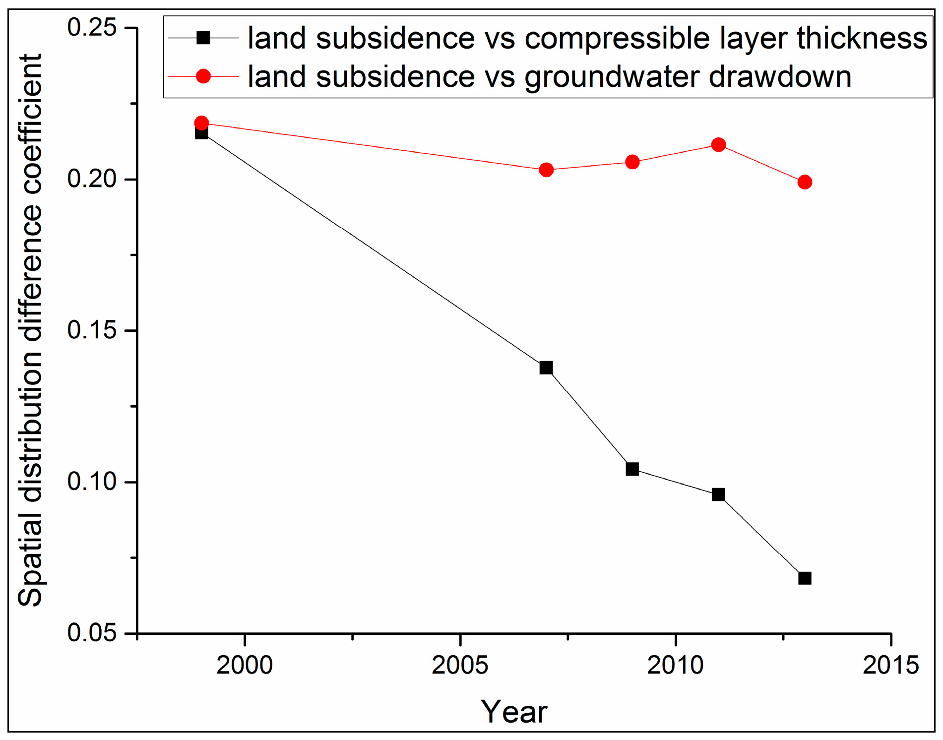
3.4. Spatial Differentiation Coefficient Comparison Analysis

The spatial differentiation coefficient between coverage areas can determine their spatial differential degree. The coverage area of the land subsidence weighted SDE fluctuated from 1999 to 2013 (Table 5). It almost covered four of the five funnels, except for Shahe-Baxianzhaung, whose development intensity was high, but was located along the direction of minor axis and close to the gravity center. Therefore, it had little influence in the spatial pattern, comparatively. The coverage area of the groundwater drawdown weighted SDE fluctuated from 1995 to 2013. Since 2007, it was maintained at about 2700 km², and the smallest appeared in 2013, associated with the precipitation peak of the previous year. The coverage area of the compressible layer thickness weighted SDE was roughly less than that of groundwater drawdown, and larger than that of land subsidence.

The spatial differentiation coefficient between the cumulative subsidence and groundwater drawdown moved up and down between 0.20 and 0.22; and that between the cumulative subsidence and the compressible layer thickness gradually decreased from 0.22 in 1999 to 0.07 in 2013 (Figure 10). This meant that (1) the spatial pattern of land subsidence is different with that of groundwater drawdown, but their difference degree is stable; and (2) the spatial pattern of land subsidence was increasingly close to that of the compressible layer. It can, therefore, be inferred that (1) land subsidence was triggered by groundwater drawdown, but confined and diversified by the compressible sediments in spatial magnitude and extent; and (2) the extent of land subsidence approached the extent of the compressible layer distribution area. Whether the land subsidence in the whole area might hit a plateau after its strong growth, or keep expanding, it needs further observations and confirmation. Continuous attention to this point is very necessary.

4. Discussion

Our study made an attempt to introduce geographic distribution measuring methods into land subsidence synthetic research. It is a geographical approach to evaluate land subsidence, groundwater drawdown, and compressible layer thickness from multiple perspectives, including point (gravity center), line (major axes), and polygon (coverage) views. The compressible sediment is a typical type of natural endowment, invariable in a long time scale and providing the material basis of land subsidence. Its non-uniform distribution can accelerate or decelerate the development of land subsidence, unbalancing the starting point of spatial evolvement of land subsidence. Groundwater drawdown is mainly caused by artificial extraction, which is a typical type of anthropogenic activity. It is the inherent drive and its spatial diversity induces unbalanced development of land subsidence. According to Krugman’s theory [47], the compressible sediment and groundwater drawdown can be regarded as the “first nature” and the “second nature”. Therefore, it is of significance to understand regional land subsidence from a geographic view. In addition, it is a benefit that the method can be implemented by using the reliable commercial GIS software ArcGIS (ESRI, Redlands, CA, USA), which provides a wide variety of spatial analysis interfaces, and allows us to focus on the geographic distribution measured in the GIS environment.

Our result distinguished the spatial distribution differences between land subsidence, groundwater drawdown, and compressible layer thickness. They suggest that (1) land subsidence developed from the southwest to the northeast and has the same concentration trend to groundwater drawdown; (2) land subsidence was stable in extent, but increasing in magnitude; and (3) with the increasing intensity, the spatial pattern of land subsidence was more similar to that of the compressible layer. This can reflect that land subsidence in Beijing is triggered by groundwater overexploitation and influenced by spatial heterogeneity of compressible layers. This is in good agreement with the conclusions from Jia et al. [21] and Zhu et al. [23].

We quantified the development center, principle orientation, dispersion, and tracking of the spatial distribution characteristics of relative study subjects. This can be achieved thanks to the ongoing multiple monitoring data based on groundwater level surveying, and ground-based geological and geodetic measurements, which enable us to acquire sufficient data and draw a scientific conclusion. However, conventional technologies cannot meet the needs of both spatial and temporal resolutions such that we can only focus on general trends, neglecting seasonal variations and funnel features. For instance, only yearly spatial distribution characteristics of land subsidence can be detected owing to the high cost of leveling; groundwater drawdown does not fully explain land subsidence, considering the heterogeneity of specific storage. In this context, remote sensors bring useful information. The InSAR technique can be used to detect land subsidence with higher spatiotemporal resolutions [48,49,50,51,52]. The Gravity Recovery and Climate Experiment (GRACE) technique can reveal the large-scale time series water storage change and the groundwater storage loss [53,54]; most notably, it has a potential to detect heterogeneous groundwater storage variations at the subregional scale, smaller than the typical GRACE footprint (200,000 km²) [55], and to detect anthropogenic signals over regions with high levels of groundwater consumption [56]. Beijing will receive about 1 × 10⁹ m³ of water through the south-to-north water diversion project and the northern part of Beijing Plain is designed for groundwater recharge. Meanwhile, ongoing urbanization will change the underlying surface condition which can decrease the quantity of precipitation infiltration. Under the above context, groundwater drawdown and land subsidence will take on a different spatial development and pattern. Our study will provide a good reference.

5. Conclusions

This paper proposed a comprehensive geographic measurement to improve the understanding of spatiotemporal distribution features of land subsidence, groundwater drawdown, and compressible layer thickness in Beijing Plain.

Land subsidence, groundwater drawdown, and compressible layer thickness were all concentrated in Chaoyang District. The concentration of land subsidence moved from southwest to northeast, which was basically consistent with groundwater drawdown. The compressible layer thickness was concentrated in the east-central Chaoyang District on, or close to, the alluvial-pluvial fan-fringe areas with mass compressible deposits.

The principle direction of land subsidence was SE–NE. It changed with that of the groundwater drawdown, but was getting closer to that of the compressible layer. The length ratio between the major and minor axes suggested that the dispersion tendency of the land subsidence became closer to that of the compressible layer with its increasing development intensity. The spatial contraction of the ellipse suggested the Chaoyang District, in the central region of the study area, experienced more serious subsidence than that in the surrounding areas most of the time.

The spatial distribution difference between land subsidence and groundwater drawdown was about 0.2, and that between land subsidence and compressible layer thickness decreased from 0.22 to 0.07, reflecting that the spatial pattern of land subsidence was increasingly close to the spatial distribution pattern of the compressible layer. Depending on development trends, the spatial pattern of land subsidence in the whole area might reach a plateau after its strong growth, which needs further study.

Generally speaking, land subsidence continued to develop with the groundwater drawdown, and its development was characterized by the inheritance owing to the compressible layer. They enabled the concentration trend of land subsidence in Beijing Plain to change little, and the spatial distribution difference remained stable. This paper focuses on the general distribution features of land subsidence, groundwater drawdown, and compressible layer thickness using GIS methods. If more detailed information on land subsidence and groundwater drawdown can be derived by cutting-edge remote sensing technologies, their distribution features can be finely depicted by the adopted methods, and the results will be more accurate and practical. Meanwhile, the error and reliability of the geographic measurement results will be broadly acceptable with the improvement of the temporal and spatial resolution of the collected monitoring datasets. Geographic distribution measurement approaches enriched the methodologies for studying land subsidence. This study will help in risk assessment of land subsidence under the “new normal” of south-to-north water diversion in Beijing Plain.

References

1. Galloway, D.L.; Burbey, T.J. Review: Regional land subsidence accompanying groundwater extraction. Hydrogeol. J. 2011, 19, 1459–1486. [Google Scholar] [CrossRef]
2. Gambolati, G.; Teatini, P. Geomechanics of subsurface water withdrawal and injection. Water Resour. Res. 2015, 51, 3922–3955. [Google Scholar] [CrossRef]
3. Calderhead, A.I.; Therrien, R.; Rivera, A.; Martel, R.; Garfias, J. Simulating pumping-induced regional land subsidence with the use of InSAR and field data in the Toluca valley, Mexico. Adv. Water Resour. 2011, 34, 83–97. [Google Scholar] [CrossRef]
4. Shi, X.Q.; Fang, R.; Wu, J.C.; Xu, H.X.; Sun, Y.Y.; Yu, J. Sustainable development and utilization of groundwater resources considering land subsidence in Suzhou, China. Eng. Geol. 2012, 124, 77–89. [Google Scholar] [CrossRef]
5. Modoni, G.; Darini, G.; Spacagna, R.L.; Saroli, M.; Russo, G.; Croce, P. Spatial analysis of land subsidence induced by groundwater withdrawal. Eng. Geol. 2013, 167, 59–71. [Google Scholar] [CrossRef]
6. Raspini, F.; Loupasakis, C.; Rozos, D.; Adam, N.; Moretti, S. Ground subsidence phenomena in the delta municipality region (northern Greece): Geotechnical modeling and validation with persistent scatterer interferometry. Int. J. Appl. Earth Obs. 2014, 28, 78–89. [Google Scholar] [CrossRef]
7. Brown, S.; Nicholls, R.J. Subsidence and human influences in mega deltas: The case of the Ganges-Grahmaputra-Meghna. Sci. Total Environ. 2015, 527–528, 362–374. [Google Scholar] [CrossRef] [PubMed]
8. Mahmoudpour, M.; Khamhechiyan, M.; Nikudel, M.R.; Ghassemi, M.R. Numerical simulation and prediction of regional land subsidence caused by groundwater exploitation in the southwest plain of Tehran, Iran. Eng. Geol. 2015, 201, 6–28. [Google Scholar] [CrossRef]
9. Castellazzi, P.; Arroyo-Domínguez, N.; Martel, R.; Calderhead, A.I.; Normand, J.C.L.; Gárfias, J. Land subsidence in major cities of central Mexico: Interpreting InSAR-derived land subsidence mapping with hydrogeological data. Int. J. Appl. Earth Obs. 2016, 47, 102–111. [Google Scholar] [CrossRef]
10. Chen, M.; Tomás, R.; Li, Z.H.; Motagh, M.; Li, T.; Hu, L.Y.; Gong, H.L.; Li, X.J.; Yu, J.; Gong, X.L. Imaging land subsidence induced by groundwater extraction in Beijing (China) using satellite radar interferometry. Remote Sens.-Basel 2016, 8, 468. [Google Scholar] [CrossRef]
11. Zou, L.; Kent, J.; Lam, N.; Cai, H.; Qiang, Y.; Li, K.N. Evaluating Land Subsidence Rates and Their Implications for Land Loss in the Lower Mississippi River Basin. Water 2016, 8, 10. [Google Scholar] [CrossRef]
12. Syvitski, J.; Kettner, A.; Overeem, I.; Hutton, E.; Hannon, M.; Brakenridge, G.; Day, J.; Vörösmarty, C.; Saito, Y.; Giosan, L.; et al. Sinking deltas due to human activities. Nat. Geosci. 2009, 2, 681–686. [Google Scholar] [CrossRef]
13. Erban, L.E.; Gorelick, S.M.; Zebker, H.A. Groundwater extraction, land subsidence, and sea-level rise in the Mekong delta, Vietnam. Environ. Res. Lett. 2014, 9, 1–6. [Google Scholar] [CrossRef]
14. Sušnik, J.; Vamvakeridou-Lyroudia, L.S.; Baumert, N.; Kloos, J.; Renaud, F.G.; La Jeunesse, I. Interdisciplinary assessment of sea-level rise and climate change impacts on the lower Nile delta, Egypt. Sci. Total Environ. 2015, 503–504, 279–288. [Google Scholar] [CrossRef] [PubMed] [Green Version]
15. Yin, J.; Yu, D.P.; Wilby, R. Modelling the impact of land subsidence on urban pluvial flooding: A case study of downtown Shanghai, China. Sci. Total Environ. 2016, 544, 744–753. [Google Scholar] [CrossRef] [PubMed] [Green Version]
16. Hoffmann, J.; Zebker, H.A.; Galloway, D.L.; Amelung, F. Seasonal subsidence and rebound in Las Vegas valley, Nevada, observed by synthetic aperture radar interferometry. Water Resour. Res. 2001, 37, 1551–1566. [Google Scholar] [CrossRef]
17. Bell, J.W.; Amelung, F.; Ramelli, A.R.; Blewitt, G. Land subsidence in Las Vegas, Nevada, 1935–2000: New geodetic data show evolution, revised spatial patterns, and reduced rates. Environ. Eng. Geosci. 2002, 8, 155–174. [Google Scholar] [CrossRef]
18. Teatini, P.; Tosi, L.; Strozzi, T.; Carbognin, L.; Wegmüller, U.; Rizzetto, F. Mapping regional land displacements in the Venice coastland by an integrated monitoring system. Remote Sens. Environ. 2005, 98, 403–413. [Google Scholar] [CrossRef]
19. Teatini, P.; Ferronato, M.; Gambolati, G.; Gonella, G. Groundwater pumping and land subsidence in the Emilia-Romagna coastland, Italy: Modeling the past occurrence and the future trend. Water Resour. Res. 2006, 42, W01406. [Google Scholar] [CrossRef]
20. Anderssohn, J.; Wetzel, H.U.; Walter, T.R.; Motagh, M.; Djamour, Y.; Kaufmann, H. Land subsidence pattern controlled by old alpine basement faults in the Kashmar valley, northeast Iran: Results from InSAR and levelling. Geophys. J. Int. 2008, 174, 287–294. [Google Scholar] [CrossRef]
21. Jia, S.M.; Wang, H.G.; Zhao, S.S.; Luo, Y. A tentative study of the mechanism of land subsidence in Beijing. City Geol. 2007, 2, 20–26. (In Chinese) [Google Scholar]
22. Zhang, Y.Q.; Gong, H.L.; Gu, Z.Q.; Wang, R.; Li, X.J.; Zhao, W.J. Characterization of land subsidence induced by groundwater withdrawals in the plain of Beijing city, China. Hydrogeol. J. 2014, 22, 397–409. [Google Scholar] [CrossRef]
23. Zhu, L.; Gong, H.L.; Li, X.J.; Wang, R.; Chen, B.B.; Dai, Z.X.; Teatini, P. Land subsidence due to groundwater withdrawal in the northern Beijing plain, China. Eng. Geol. 2015, 193, 243–255. [Google Scholar] [CrossRef]
24. Galloway, D.L.; Hudnut, K.W.; Ingebritsen, S.E.; Phillips, S.P.; Peltzer, G.; Rogez, F.; Rosen, P.A. Detection of aquifer system compaction and land subsidence using interferometric synthetic aperture radar, Antelope Valley, Mojave Desert, California Water. Resour. Res. 1998, 34, 2573–2585. [Google Scholar] [CrossRef]
25. Mitchell, A. The ESRI Guide to GIS Analysis Volume 2: Spatial Measurements & Statistics; ESRI Press: Redlands, CA, USA, 2005; pp. 21–61. [Google Scholar]
26. Li, X.B. Visulizing spatial equality of development. Sci. Geogr. Sin. 1999, 19, 254–257. (In Chinese) [Google Scholar]
27. Xu, J.H.; Yue, W.Z. Evolvement and comparative analysis of the population center gravity and the economy gravity center in recent twenty years in china. Sci. Geogr. Sin. 2001, 21, 385–389. (In Chinese) [Google Scholar]
28. Lefever, D.W. Measuring geographic concentration by means of the standard deviational ellipse. Am. J. Soc. 1926, 32, 88–94. [Google Scholar] [CrossRef]
29. Furfey, P.H. A note on Lefever’s “standard deviational ellipse”. Am. J. Soc. 1927, 33, 94–98. [Google Scholar] [CrossRef]
30. Warntz, W.; Neft, D. Contributions to a statistical methodology for areal distributions. Reg. Sci. 2006, 2, 47–66. [Google Scholar] [CrossRef]
31. Robert, S. The standard deviational ellipse; an updated tool for spatial description. Geogr. Ann. 1971, 53, 28–39. [Google Scholar]
32. Wang, B.; Shi, W.Z.; Miao, Z.L. Confidence analysis of standard deviational ellipse and its extension into higher dimensional Euclidean space. PLoS ONE 2015, 10, e0118537. [Google Scholar] [CrossRef] [PubMed]
33. Bashshur, R.L.; Metzner, C.A. The application of three-dimensional analogue models to the distribution of medical care facilities. Med. Care 1970, 8, 395–407. [Google Scholar] [CrossRef] [PubMed]
34. Vanhulsel, M.; Beckx, C.; Janssens, D.; Vanhoof, K.; Wets, G. Measuring dissimilarity of geographically dispersed space-time paths. Transportation 2011, 38, 65–79. [Google Scholar] [CrossRef]
35. Yue, T.X.; Fan, Z.M.; Liu, J.Y. Changes of major terrestrial ecosystems in China since 1960. Glob. Planet. Chang. 2005, 48, 287–302. [Google Scholar] [CrossRef]
36. Li, C.; Liu, J.P.; Liu, Q.F.; Yu, Y. Dynamic change of wetland landscape patterns in Songnen plain. Wetl. Sci. 2008, 6, 167–172. (In Chinese) [Google Scholar]
37. Wang, B.J.; Shi, B.; Inyang, H.I. GIS-based quantitative analysis of orientation anisotropy of contaminant barrier particles using standard deviational ellipse. Soil Sediment Contam. 2008, 17, 437–447. [Google Scholar]
38. Mamuse, A.; Porwal, A.; Kreuzer, O.; Beresford, S. A new method for spatial centrographic analysis of mineral deposit clusters. Ore Geo. Rev. 2009, 36, 293–305. [Google Scholar] [CrossRef]
39. Eryando, T.; Susanna, D.; Pratiwi, D.; Nugraha, F. Standard Deviational Ellipse (SDE) models for malaria surveillance, case study: Sukabumi district-Indonesia, in 2012. Malar. J. 2012, 11. [Google Scholar] [CrossRef]
40. O’Loughlin, J.; Witmer, F.D.W. The localized geographies of violence in the north Caucasus of Russia, 1999–2007. Ann. Assoc. Am. Geogr. 2011, 101, 178–201. [Google Scholar] [CrossRef]
41. Zhao, L.; Zhao, Z.Q. Projecting the spatial variation of economic based on the specific ellipses in China. Sci. Geogr. Sin. 2014, 34, 979–986. (In Chinese) [Google Scholar]
42. Peng, J.; Chen, S.; Lü, H.L.; Liu, Y.X.; Wu, J.S. Spatiotemporal patterns of remotely sensed PM 2.5, concentration in China from 1999 to 2011. Remote Sens. Environ. 2016, 174, 109–121. [Google Scholar] [CrossRef]
43. Jia, S.M.; Ye, C.; Liu, J.R.; Zhao, S.S.; Wang, R.; Yang, Y.; Wang, H.G.; Dong, D.W. Investigation of Land Subsidence in Beijing; Beijing Institute of Hydrogeology and Engineering Geology: Beijing, China, 2006; p. 5. (In Chinese) [Google Scholar]
44. Liu, Y.; Ye, C.; Jia, S.M. Division of water-bearing zones and compressible layers in Beijing’s land subsidence areas. City Geol. 2007, 2, 10–15. (In Chinese) [Google Scholar] [CrossRef]
45. Beijing Water Authority, Government Affairs, Statistical Information. Available online: http://www.bjwater.gov.cn/pub/bjwater/zfgk/tjxx/ (accessed on 5 May 2016).
46. Griffith, D. Theory of Spatial Statistics. In Spatial Statistics and Models; Gaile, G.L., Willmott, C.J., Eds.; D. Reidel Publishing Company: Dordrecht, The Netherlands, 1984; pp. 3–15. [Google Scholar]
47. Krugman, P. First nature, second nature, and metropolitan location. Reg. Sci. 1993, 33, 129–144. [Google Scholar] [CrossRef]
48. Chen, F.; Lin, H.; Yeung, K.; Cheng, S.L. Detection of Slope Instability in Hong Kong Based on Multi-baseline Differential SAR Interferometry Using ALOS PALSAR Data. GISci. Remote Sens. 2010, 47, 208–220. [Google Scholar] [CrossRef]
49. Ng, H.M.; Ge, L.L.; Li, X.J.; Abidin, H.Z.; Andreas, H.; Zhang, K. Mapping land subsidence in Jakarta, Indonesia using persistent scatterer interferometry (PSI) technique with Alos Palsar. Int. J. Appl. Earth Obs. 2012, 18, 232–242. [Google Scholar] [CrossRef]
50. Strozzi, T.; Teatini, P.; Tosi, L.; Wegmüller, U.; Werner, C. Land subsidence of natural transitional environments by satellite radar interferometry on artificial reflectors. Geophys. Res. Earth Surf. 2013, 118, 1177–1191. [Google Scholar] [CrossRef]
51. Samsonov, S.V.; D’Oreye, N.; González, P.J.; Tiampo, K.F.; Ertolahti, L.; Clague, J.J. Rapidly accelerating subsidence in the greater Vancouver region from two decades of ERS-ENVISAT-RADARSAT-2 DInSAR measurements. Remote Sens. Environ. 2014, 143, 180–191. [Google Scholar] [CrossRef]
52. Dehghan-Soraki, Y.; Sharifikia, M.; Sahebi, M.R. A comprehensive interferometric process for monitoring land deformation using ASAR and PALSAR satellite interferometric data. GISci. Remote Sens. 2015, 52, 58–77. [Google Scholar] [CrossRef]
53. Yeh, P.J.-F.; Swenson, S.C.; Famiglietti, J.S.; Rodell, M. Remote sensing of groundwater storage changes in Illinois using the Gravity Recovery and Climate Experiment (GRACE). Water Resour. Res. 2006, 42, W12203. [Google Scholar] [CrossRef]
54. Wang, X.W.; de Linage, C.; Famiglietti, J.; Zender, C.S. Gravity Recovery and Climate Experiment (GRACE) detection of water storage changes in the Three Gorges Reservoir of China and comparison with in situ measurements. Water Resour. Res. 2011, 47, W12502. [Google Scholar] [CrossRef]
55. Huang, Z.Y.; Pan, Y.; Gong, H.L.; Yeh, P.J.-F.; Li, X.J.; Zhou, D.M.; Zhao, W.J. Subregional-scale groundwater depletion detected by GRACE for both shallow and deep aquifers in North China Plain. Geophys. Res. Lett. 2015, 42, 1791–1799. [Google Scholar] [CrossRef]
56. Pan, Y.; Zhang, C.; Gong, H.L.; Yeh, P.J.-F.; Shen, Y.J.; Guo, Y.; Huang, Z.Y.; Li, X.J. Detection of human-induced evapotranspiration using GRACE satellite observations in the Haihe River basin of China. Geophys. Res. Lett. 2016, 43. [Google Scholar] [CrossRef]
Figure 1. Location, type of main sediments, and digital elevation model of the study area.
Water 09 00064 g001
Figure 2. Cumulative land subsidence in Beijing Plain. For simplicity, only three of six collected datasets are shown, and the others are shown in Figure S1.
Water 09 00064 g002
Figure 3. Compressible layer thickness.
Water 09 00064 g003
Figure 4. Groundwater seepage field. For simplicity, only three of six collected datasets are shown, and the others are shown in Figure S2.
Water 09 00064 g004
Figure 5. Discrete point set of land subsidence.
Water 09 00064 g005
Figure 6. Space expression of the standard deviational ellipse (SDE): (a) basic parameters and (b) distribution difference [41].
Water 09 00064 g006
Figure 7. Gravity center of cumulative land subsidence, groundwater drawdown, and the compressible layer.
Water 09 00064 g007
Figure 8. The 2001–2015 yearly time series precipitation, and groundwater storage anomalies in Beijing Plain. Note that these data were retrieved from the Beijing Water Resources Bulletin from 2001 to 2015 [45] issued by the Beijing Water Authority.
Water 09 00064 g008
Figure 9. SDE of cumulative land subsidence, groundwater drawdown, and compressible layer thickness. The map on the left shows SDE of land subsidence; the map on the right shows SDE of water drawdown.
Water 09 00064 g009
Figure 10. Spatial distribution difference coefficient.
Water 09 00064 g010