1. Introduction
Nitrogen (N) losses from point (PS) and diffuse sources (NPS) are recognized to be the leading causes of water body impairment throughout Europe [
1]. Despite improvements of water quality in recent years, many aquatic ecosystems in Europe are still at risk of eutrophication from excessive N concentrations [
2,
3]. Agriculture has been estimated to contribute around 55% of the N loads reaching the European seas while point sources are responsible for around 25% [
4]. The European key policy instrument to protect inland (surface and groundwater), transitional and coastal water resources is the Water Framework Directive (WFD) [
5]. The European Commission established ecological objectives for all European waters, aiming at more integrated and coherent approach for water protection. The WFD complemented two major pieces of legislations that were put in place in the early 1990s to control the amount of nutrient pollution of European waters, i.e., the Nitrates Directive [
6] and the Urban Waste Water Treatment Directive [
7]. The Nitrates Directive regulates the emission of Nitrogen in the form of Nitrate (N-NO
3) from agricultural activities by setting manure application limits, and prescribes the implementation of action programs in Nitrate vulnerable zones. The Urban Waste Water Treatment Directive requires all Member States to implement efficient wastewater treatment and establishes wastewater to undergo at least secondary treatment (C-plants) when discharged into sensitive areas. After 25 years of implementation, many problems linked to high Nitrate concentrations still affect a large number of water bodies in Europe.
Developing efficient management strategies to fulfill the EU legislation requirements needs to consider simultaneously point and diffuse sources of Nitrate. Point source emissions in practice are easy to control as their location and characteristics are well known. Changing the treatment level of a wastewater treatment plant (WWTP) has an immediate effect on the discharged water quality. On the other hand, nonpoint sources are more difficult to control due to their diffuse nature. Furthermore, there is usually a lag time between the implementation of a remedial measure and the environmental response [
8].
Management strategies should also consider the location of sources of pollution in order to choose the most appropriate conservation strategies that will achieve the required environmental targets, while being economically and socially viable. A targeted implementation of Best Management Practices (BMPs) at selected locations in a watershed has been recognized as an effective strategy to improve water quality [
9]. The state of the art approach is thus to design a local specific BMPs strategy [
10]. However, this could lead to a multiplication of the implementation of many BMPs in the watershed, without ensuring that the environmental targets at the watershed outlet are achieved [
11]. Interactions between BMPs may also significantly affect their individual performances at a watershed scale. Harrell and Ranjithan [
12] emphasized that a reduced number of management practices could achieve the same outcomes as a multitude of measures implemented throughout the watershed.
Since management practices are usually implemented under a limited budget, costs associated with unnecessary/redundant management actions may jeopardize attainability of designated water quality goals. Consideration of the implementation and maintenance costs of each conservation strategy is essential for the identification of effective management strategies, and to increase the acceptability of the selected measures. Thus, a balance has to be achieved between the environmental and economic implications of the many possible conservation strategies. While it is always desirable to implement a BMP that costs the least and gives the most reduction in pollutant load, win-win solutions are few and far between, and the environmental targets can only be achieved through the appropriate combinations of spatially, temporally and economically tailored sets of conservation measures [
13,
14]. When several management practices are to be considered together across a watershed, the identification of efficient conservation strategies becomes a spatial multi-criteria optimization problem. Spatial optimization of land use and conservation practices under various objective functions/constraints can help sustainably manage limited resources [
14,
15,
16,
17,
18,
19].
Evolutionary optimization methods such as genetic algorithms [
20] are popular in spatial optimization [
18,
19,
20,
21,
22,
23,
24]. The most frequent method of spatial optimization is to link dynamically a watershed simulation model with an optimization algorithm [
18,
19,
24,
25,
26,
27], wherein watershed model outputs are used to estimate the objective functions of the optimization algorithm. The Soil and Water Assessment Tool (SWAT, [
28,
29]) is a watershed model commonly used to simulate the impact of land use and land management changes on water quantity and water quality [
28]. Interest has grown in spatial optimization of conservation practices using genetic algorithms and SWAT (e.g., [
18,
19,
23,
24]). Most of the previous works have focused either on using a single objective function for optimization that combines BMP effectiveness with cost [
15,
21] or on sequential optimization of effectiveness and cost as separate objective functions [
30,
31], i.e., constraining one objective function during optimization of the other. In contrast, simultaneous optimization of economic and environmental objectives allows identifying trade-off strategies [
18,
23,
24]. Furthermore, none of these studies considered both point and diffuse sources, while it is possible that the most efficient strategies would consider a combination of BMPs that target either type of pollution.
The overall goal of this work was to explore potential gains in searching cost-effective solutions to reduce N-NO
3 pollution in the large Upper Danube Basin (132,000 km
2) by considering both point and diffuse sources. The Basin is characterized by the highest values of N-NO
3 concentration in the surface water in the entire Danube [
32], thus Nitrate pollution abatement in the region appears crucial to restore the good ecological status of the Danube River [
33]. We hypothesize that important reductions of N-NO
3 in the river network can be achieved at affordable cost by applying spatial targeting approaches to identify optimal conservation practice combinations. We used SWAT to simulate point and diffuse N-NO
3 emissions and fate in a watershed. Starting from current basin conditions, we first analyzed the impact of single conservation measures applied uniformly across the region (iterative simulations) to assess maximum N-NO
3 abatement level that could be reached. We then ran multi-objective, spatially explicit optimization routines to search for solutions that considered several conservation actions in different parts of the Basin.
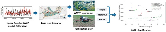
3. Methodology
The analysis was conducted with the R-SWAT-DM framework [
36]. R-SWAT-DM is an integrated tool that enables spatially explicit decision-making, helping stakeholders to better understand the main water quality problems and finding the most efficient practices for a given watershed. The framework assesses the economic and water quality impacts of different types/levels of management practices and compares them with the Baseline Scenario (BLS). It applies different BMPs at different location, thus allowing the evaluation of their overall impact and search for spatial combinations that are most appropriate to improve the water quality at a minimum cost.
Users can run single or combined simulations of spatially explicit management practices, or iterative simulations whereby all management practices of one type are changed simultaneously step-wise in a fixed range of values. Alternatively, they can also choose to run a multi-objective optimization process. In this case, users should specify the environmental objective, choosing among the available options, the management practices to be considered. Once the simulation and/or optimization process has finished, the user can analyze and compare the management scenario outputs graphically and statistically. The framework can also generate maps with detailed spatial information about a selected scenario.
The framework includes the following main components: (1) a watershed biophysical model (SWAT) for simulating hydrologic and water quality processes under current conditions and management scenarios; (2) an economic module to estimate the monetary value of each management scenario; and (3) an optimization engine to search for trade-off management scenarios according to environmental and socioeconomic objectives. The framework can model nutrient reduction measures related to both PS (WWTP upgrading) and NPS (crop fertilization and irrigation strategies).
The steps of the analysis for the Upper Danube Basin were: (1) set up SWAT model to simulate N-NO3 fluxes under baseline (BLS) and alternative management scenarios; (2) define environmental and economic objectives; (3) apply a multi-objective simulation/optimization tool; (4) perform a sensitivity analysis for the most relevant components of model; and (5) identify optimal spatial allocation of best nutrient management practices.
3.1. Biophysical Model Description
SWAT [
29] was used to assess the impact of point sources and land use management practices on N-NO
3 fluxes and on agricultural yields. The SWAT model integrates all relevant eco-hydrological processes including water flow, surface runoff, percolation, lateral flow, groundwater flow, evapotranspiration, transmission losses, nutrients and sediments, vegetation growth, land use, and water management. The simulation of watershed hydrology with SWAT is divided into two main phases: the land phase and the routing phase of the hydrologic cycle, which controls the amount of water, sediment, and nutrients into the main stream network. Essentially, SWAT uses the water balance approach to simulate watershed hydrologic partitioning [
29]. Watersheds are divided into spatially linked subbasins; the subbasins are divided into Hydrological Response Units (HRUs) with unique soil/land use and slope characteristics. The land phase is solved at HRU level, which determines water flow and nutrient load outputs; these outputs are routed through the subbasin and subsequently, in the water phase, through the stream network till the watershed outlet.
SWAT set-up for the Upper Danube Basin comprised several sources: (a) Digital Elevation Map (DEM) of 100 × 100 m, obtained from the Catchment Characterization Modeling version 2 (CCM2) DEM [
37]; (b) soil map of 1 × 1 km, obtained from the Harmonized World Soil Database (HWSD) [
38]; (c) watershed and stream delineation, based on the CCM2 database for continental Europe [
37]; and (d) EFAS-METEO climate data including daily precipitation, temperature, solar radiation, wind speed and relative humidity with spatial resolution of 25 km [
39].
A land use map of 1 × 1 km for year 2000 was built from the combination of databases [
40,
41,
42,
43]. In the subbasins with dominant arable land, the crops were distributed according to the EUROSTAT [
44] crop statistics at district level (NUTS 2) using an ad hoc land use assignation routine. The Upper Danube was discretized into 753 subbasins ranging in size from 3 ha to 1011 km
2, with an average area of 143 km
2. From the combination of land use, soils and slopes, 822 HRUs were defined, 75 of which were urban areas [
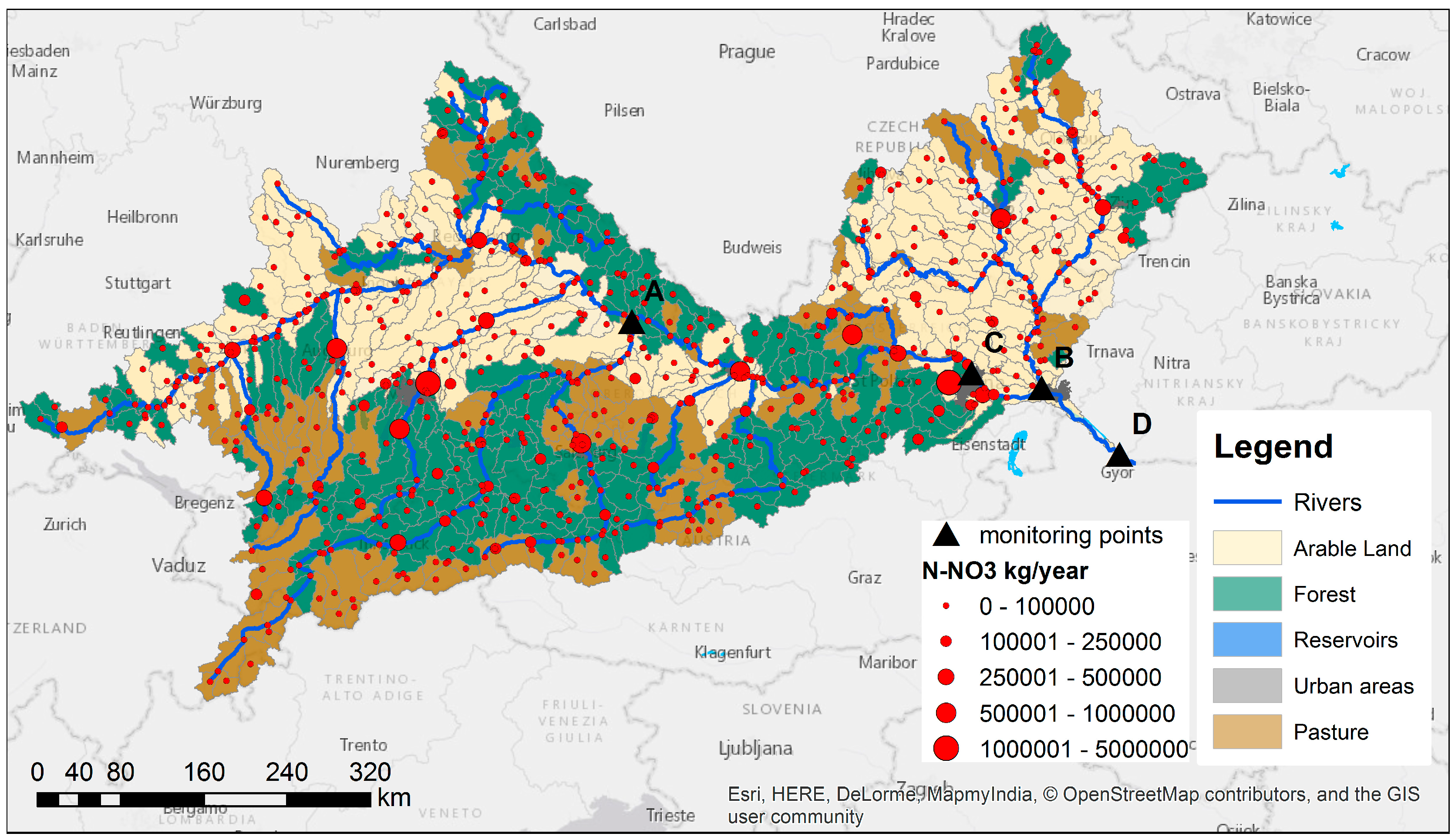
45]. Point sources were defined in 533 sub-basins (more than 70% of all subbasins) using the European waste water treatment database WWTPD [
46] (
Figure 1). In the SWAT model only one single point source can be defined per subbasin; hence a point source represents all the point sources comprised in the subbasin.
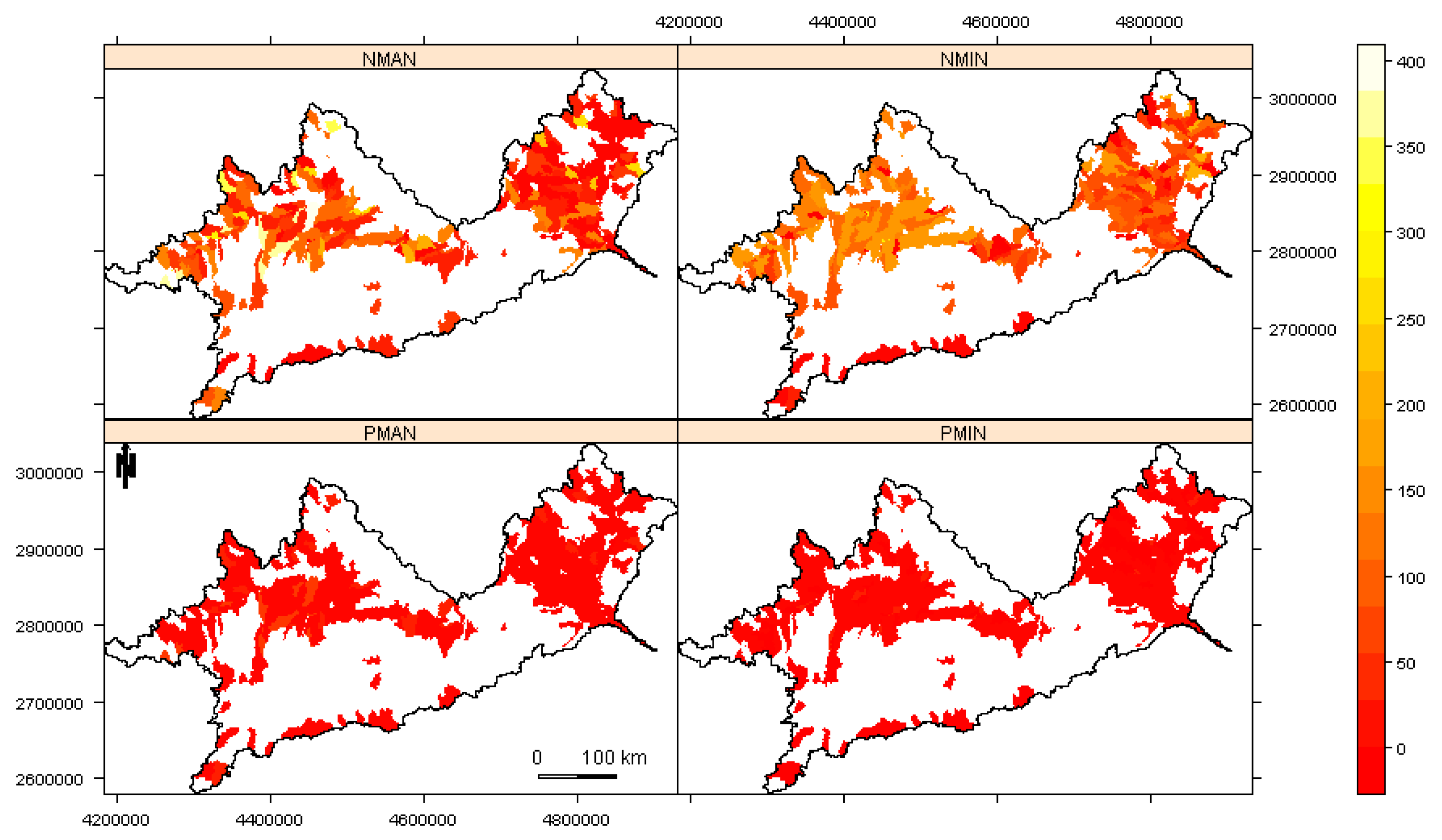
Crop management operations were based on the heat units approach that were calculated at regional level as detailed in Wriedt et al. [
47]. Fertilization was based on outputs from the CAPRI model [
40]. All arable land (291 HRUs) was fertilized, however the main fertilized crops were annual row crops, winter and summer cereals, and managed pastures (
Table 1). Fertilization management practices (type and schedule) were based on SWAT literature and SWAT database of fertilizers [
28] adapted to the European context [
48].
Figure 2 shows the applied fertilization patterns used in the BLS scenario. The irrigated area covers only around 700 km
2; the auto irrigation option was selected using the irrigated areas from national statistics. Since the irrigated land in the region was small, irrigation management practices were not further considered in the case study.
The model was calibrated in steps: calibration of crop yields, multi-site calibration of streamflow, and calibration of N-NO
3 at the outlet of the watershed. Annual simulated crop yields for 1995–2009 were calibrated by manually adjusting three parameters (the crop harvest index, HVSTI, and the optimal and minimum plant growth, T_OPT and T_BASE, respectively) to match yields reported by EUROSTAT [
44] (
Table 1). SWAT crop yields were generally well captured, albeit some differences were noticeable for generic agricultural crop, corn, corn silage, and soybean, probably due to very productive crop varieties cultivated in the Basin. However, given that sensitive crop management inputs [
49] such as planting and harvesting time, fertilizer and irrigation water inputs were generalized for application in the large Basin rather than be locally defined, calibration of crop yields was considered satisfactory.
Monthly streamflow was calibrated in 98 gauged stations for the period 1995–2006, and validated in 150 gauged stations for the period 1995–2009. With reference to the calibrated dataset, streamflow simulation at more than 50% of stations had an average percent bias (PBIAS%, [
50]) of 11% and Nash Sutcliffe efficiency (NSE, [
50]) of 0.57. For the validation dataset, the PBIAS% was satisfactory for more than 60% of gauged stations (average values of 9.7%) and for these the average Nash Sutcliffe was around 0.53. More details about the model setup and the calibration procedure can be found in Malagó et al. [
45]. Mean monthly N-NO
3 concentration was calibrated manually at the only station for which data was available at the time of the study, i.e., at the watershed outlet for the period 1995–2009, by changing two basin parameters: the denitrification exponential rate coefficient (CDN) was set at 0.6 and the fraction of field capacity water content above which denitrification occurs (SDNCO) was set to 1. After calibration, SWAT N-NO
3 mean concentration at the outlet (2.15 mg/L) was very close to the observation mean (2 mg/L); PBIAS% of monthly N-NO
3 simulation at the outlet was 6.8%. The calibration was validated in other 74 gauging stations in the region that became available at a later stage. SWAT simulated well the monthly N-NO
3 concentrations with performances from very good to satisfactory (PBIAS% < ±70% [
50]) in about 57% of them.
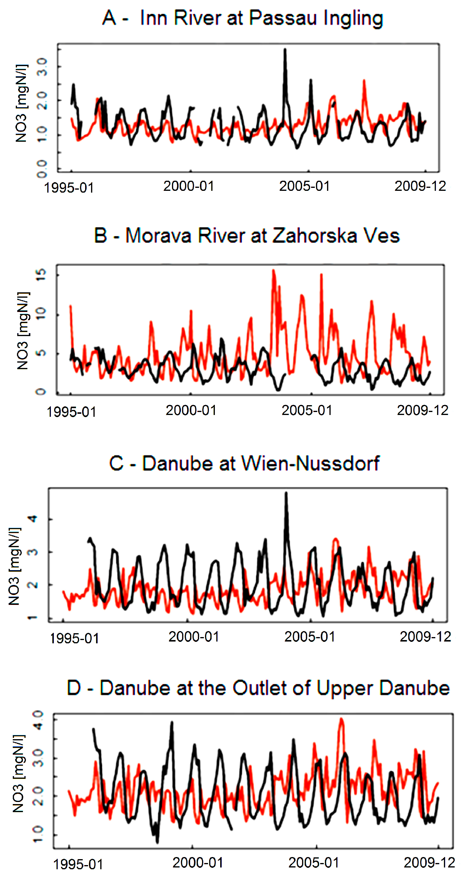
Figure 3 shows SWAT simulation and observations of N-NO
3 concentration at some key stations of the Basin.
3.2. Best Management Practices
Two groups of Nitrate Best Management Practices were considered in the work: PS and NPS BMPs. Improved sewage treatment can substantially reduce PS pollution. Primary treatment removes only bulky materials. The more expensive secondary (C-plants) treatment also removes suspended particles and part of the nutrient-rich organic material. The even more expensive tertiary treatment, for instance CN (C-removal + nitrification), CND (C-removal + nitrification + denitrification), or CNDP (C-removal + nitrification + denitrification + Phosphorus removal), which is sporadically implemented, also removes most of the dissolved nutrients. In the Upper Danube Basin, 533 urban and industrial PS were considered, which were modeled as C-plants Waste Water Treatment Plants (WWTP) [
51]. The WWTP capacity of treatment varied from 9 m
3/day to 604,500 m
3/day, with an average of 8306 m
3/day. In this work we considered two possible levels of upgrading WWTP treatment, which achieved removal of a higher percentage of nutrients at higher costs (
Table 2).
For NPS, we considered BMPs related to mineral fertilization (
Table 1). Nitrogen from mineral fertilizer is the major source of N input in EU countries and remains an important cost for the farmers. Mineral fertilization could substantially vary among HRUs, and affected the nutrient losses on one side and the yield crop on the other. It is true that Nitrogen input from manure remains important in regions of high livestock density [
52]. However, since the amount of available manure depends on livestock density, a change in manure fertilization would not be realistic without considering changes in livestock systems. Such analysis was out of the scope of this work. Therefore, in this study livestock density and manure fertilization were kept unchanged from the current situation (BLS).
3.3. Environmental Objective
Minimizing pollutant concentration or loads, or alternatively maximizing reduction of pollutant concentration, is a key objective in water pollution control management practices. There is no single way to assess the water quality in a watershed, especially when water quality is related to the concentration of various contaminants over a period of time in many geographical points. As well, there is no ideal mathematical equation to perform the aggregation of temporal and spatial pollutant concentration values in one single metric that resumes the global quality. Hence, the following three different possibilities for aggregating water quality indicators have been included in the framework.
The average pollutant concentration in all reaches for the whole simulation period.
where:
nt: number of time-steps in the simulation period.
ns: number of modeled reaches.
Qij: concentration (mg/L) of pollutant in reach “i” and simulation time-step “j”.
The cumulated contaminant: sum of contaminant concentrations in reaches that exceeded an environmentally acceptable threshold.
where
Th: threshold that is considered as environmentally acceptable. This can be set according to Water Framework Directive (WFD, [
5]) targets or ecological considerations; and the other variables are defined as in Equation (1).
The total load at the watershed outlet:
where
TLj: load of the pollutant exported at the watershed outlet in the simulation period “
j”.
3.4. Economic Objective
PS and NPS BMPs yield benefits in water quality and wildlife habitats, but their implementation and maintenance come at a cost. On the one hand, agriculture generates economic profit. It is important to consider the impact of BMPs adoption on farmers’ revenue. On the other hand, the upgrade of the WWTP is expensive (
Table 2). A priori, it is not clear where it is more efficient to invest in. The most efficient solution might well be an adequate spatial combination of different BMPs adoption. The economic objective function was defined as:
where:
TNI: is the total net income (considering together gross margin of the farmers and cost of the WWTP).
x: denotes decision variables reflecting the quantity and location (HRU) of fertilizer practices.
y: denotes decision variables reflecting the quantity and location (HRU) of irrigation practices.
z: denotes decision variables reflecting the type and location of the WWTP.
g1: is the gross margin related with the agricultural production.
g2: is the cost related to upgrading the WWTP (additional cost in relation with baseline situation).
T: is the assessment period.
: is the vector of calibrated watershed model parameters.
: represents driving forces (i.e., rainfall, temperature, and other environmental factors).
wc: is the unit cost of the implementation the conservation practice.
cr: is the unit price of beneficial products of the conservation practice.
g1(BLS): is the base line situation gross margin related with the agricultural production.
For the BLS, the WWTP cost (the g2 component) was set to zero. In the following paragraphs, the evaluations of the two economic components related to agriculture and to the WWTPs are described.
3.4.1. Component Related to Agriculture
In order to estimate farmer gross margin as affected by the different management strategies, we applied a function based on crop yield, crop price, fertilizer cost, irrigation water cost, standard operational cost, and specific fixed cost (including seeds cost, tillage operations, machinery, grain drying, labor, etc.). For each alternative BMP, total gross margin was estimated as:
where:
: agricultural total gross margin for the BMP.
: yield of crop j in HRU i under a BMP.
Aij: area (ha) of crop j in HRU i.
Upj: unit price (income €/tm) of crop
j (
Table 3).
: quantity of fertilizer applied (kg/ha) to crop j in HRU i under a BMP.
: unit cost of fertilizer (€/kg) of crop j in HRU i under a BMP.
: the water irrigation unit cost (€/mm), constant across HRUs.
: irrigation quantity (mm/ha) for crop j in HRU i under a BMP.
: operational management cost for the crop
j (
Table 3).
Crop management costs were assumed constant throughout the simulated period and independent from the annual yield. The average crop yield for the period 1995–2009 of each HRU under management scenarios was assessed with SWAT.
Table 3 includes the average, minimum and maximum selling price for all crops [
44] in the study region, and the operational (fixed) costs, including the labor, machinery. Instead, current European subsidies were not considered in farmers’ income.
N, P and K are applied with several fertilizer products (Anhydrous ammonia, Nitrogen solutions 30%, Urea 44–46, Ammonium nitrate, Sulfate of ammonium, super phosphate 20%, etc.) containing different forms and percentages of the elements. The total cost of the fertilization was estimated based on the quantity (kg) of elementary N, P and K present in the applied fertilizers. The cost per kg of N, P and K was estimated from annual data from 2000 to 2013 [
53]. The resulting prices were 1.21 € per kg of Nitrogen, 2.8 € per kg of Phosphorus and 0.97 € per kg of Potassium and the summary cost per fertilizer is showed in
Table 4.
3.4.2. Component Related to WWTP
Two upgrading options were considered (
Table 2): (i) upgrading from C-plants to CN plants (C-removal + nitrification) or (ii) upgrading to CNDP plans (C-removal + nitrification + denitrification + Phosphorus removal). Cost estimates for different upgrading options in municipal wastewater treatment plants for all Danube countries were derived from Dworak et al. [
51], using the cost data reported for Austria. The total wastewater treatment cost includes all investment costs (costs of construction and costs of the mechanical and electrical equipment) as well as all operational costs (labor costs, energy expenses, maintenance costs, chemicals expenses, sludge treatment and disposal costs, and discharge levies). To make investment and operational costs comparable, all investment costs were converted into annual values using a 20-year depreciation horizon and a 5% real interest rate. These costs were available for different sizes of the WWTP, varying from 75 to 150,000 population equivalent. We fitted a power equation to express the cost of the upgrade as a function of the volume of water treated (
Table 2). As a result, the total cost for a WWTP is expressed in €/m
3 per year.
For each WWTP scenario the total wastewater treatment cost in the basin was estimated as the sum of the treatment cost for each plant, which was based on the treatment type and the volume of water according to:
: WWTP upgrading annual cost for the mp water restoration management practices.
Qk: flow average (m3/day) in PS k.
Yk: type of upgrade of the k WWTP. 0: no upgrade; 1: upgrade from C to CN; upgrade from C to CNDP.
Coef1 [
Yk]: coefficient 1 for the
Yk WWTP type of upgrade (
Table 2).
Coef2 [
Yk]: coefficient 2 for the
Yk WWTP type of upgrade (
Table 2).
3.5. Multi-Objective Optimization Method
A logical approach for targeting PS and NPS pollution control practices should be to propose a multi-objective problem following the next equation:
Under this or other similar approaches, the objective functions are often conflicting and incommensurable. For example, implementation of a large number of conservation practices would likely result in lower pollutant loads, but the cost for implementation and maintenance of these practices would increase. Hence, the optimal solutions for any objective could substantially differ from the optimal solutions for another objective. Multi-objective optimization approaches can determine a set of non-dominated solutions belonging to a Pareto-optimal front. Non-dominated solutions are a set of solutions in the search space that are better than any other solution in one or more objective [
54]. Any improvement in one objective among Pareto-optimal solutions will essentially result in the degradation of at least another objective [
55].
Since the shape of the objective function cannot be assumed as smooth or differentiable in our management practices application problem, gradient approaches such as quasi-Newton methods cannot be applied [
56]. Instead, gradient free methods such as evolutionary algorithms are applicable as optimization method. The non-dominated sorting genetic algorithm NSGA-II [
57] is among the most commonly used multi-objective global optimization methods with numerous successful applications in watershed management [
24,
58,
59]. The procedure starts with an initial population of solutions that are typically generated randomly. The fitness of individual solution in successive generations increases through selection, crossover, and mutation. The procedure stops when a set of predefined termination conditions is met. To run a multi-objective optimization process in the R-SWAT-DM framework, the user should select at least two objectives. Usually at least one refers to the environmental objective, e.g., selecting a constituent of interest and the aggregation metric to be applied (Equations (1)–(3)). For the economic objective, the user could choose to maximize the total net income, or to minimize the investment in WWTP, or to maximize the gross margin for the farmers.
For the Upper Danube Basin, two objectives were considered. The environmental objective focused on N-NO
3 contamination, because it is the most important issue in the region [
60]. The aggregation metric was the sum of NO
3 concentration exceeding the WFD threshold of 50 mg/L in all reaches (Equation (2)). However, the total N-NO
3 load at the watershed outlet (Equation (3)) is a key indicator of water quality [
33], thus optimization was constrained to not exceed BSL level. The economic objective was the total net income as defined in Equation (4).
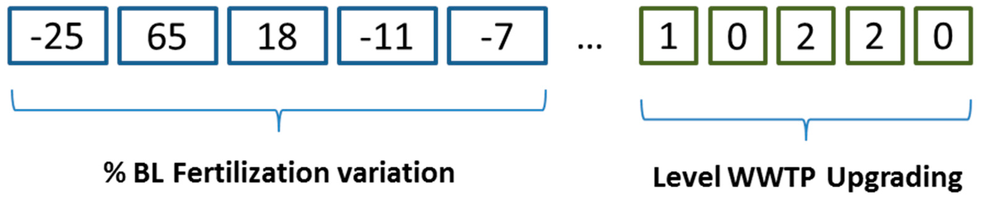
The multi-objective optimization module simulates individuals of a population as chromosomes (scenarios), which in turn contain genes, i.e., the single units for which conservation can be applied, as their building blocks. Each gene represents a particular set of BMPs (BMP combination) on the chromosome encoding a specific trait. In the Upper Danube Basin, the unit for controlling diffuse pollution was the single HRU. There were 291 fertilized HRU, while we neglected the irrigation option. For point source pollution, the unit was the single WWTP. Therefore, chromosomes for the Upper Danube Basin consisted of 291 HRU + 533 WWTP genes (
Figure 4).
The NSGA-II results are very sensitive to the operational parameters (population size, number of generations, crossover, and mutation rates) that define the search algorithm. As described in Maringanti et al. [
23], a nonlinear sensitivity analysis where operational parameters were incremented one at a time was conducted to define the NSGA-II best population size, number of generations, mutations, and crossover probabilities.
4. Results and Discussion
The Baseline Scenario (BLS) shows the current state of the Upper Danube basin according to the model of SWAT. The simplest analysis that can be performed with the R-SWAT-DM framework is to simulate one single spatially explicit conservation strategy, in order to know its economic and environmental outcomes.
Table 5 show a short description of the management strategies analyzed in this paper.
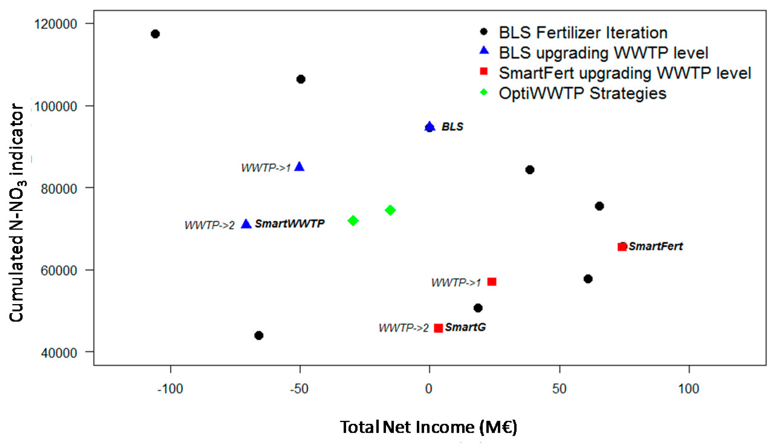
Next, results were obtained running the tool to simulate iterative changes in the rate of mineral fertilization applied uniformly in all HRUs (black dots in
Figure 5). The iterative simulations showed that when starting from a very low rate of mineral fertilizer applied (for all HRUs), a fertilization increase causes low pollution increase while the total net income increases sensibly as crop yields incomes increase more than fertilizer costs. It is possible to identify an optimal fertilization rate (SmartFert point in
Figure 5) corresponding to the maximum total net income. Once this fertilization rate is exceeded, total net income starts to decrease, while pollution continues to increase. Compared to the BLS, the SmartFert strategy corresponds to a reduction of 35% in mineral fertilizer rate applied, and results in an increment of total net income of 75 M€ and in a 30% reduction of cumulated N-NO
3 pollution (
Table 6). SmartFert results are in line with the outcomes of the analysis of statistics and agri-environmental indicators available for the four involved Countries from Eurostat [
61]. These indicators point out a systematic potential surplus of Nitrogen on agricultural land: a surplus of 90, 86, 33, and 30 kg/ha/year is reported for year 2008, respectively, for Germany, Czech Republic, Austria and Slovakia that correspond to 42%, 50%, 25% and 28% of total Nitrogen inputs. Surplus numbers are clearly in line with the suggested reduction rates identified in the SmarFert scenario.
Iterative simulations of WWTP consists of upgrading all WWTP by one (to CN; WWTP => 1), or two levels (to CNDP, WWTP => 2;
Figure 5). The total cost of upgrading all plants at CN level is 50 M€, and to CNDP level is of 71 M€ (SmartWWTP), achieving approximately pollution reductions of 10% and 26%.
The analysis can be done starting from the BLS situation (blue triangles) or from the SmartFert strategy (red squares). Remarkably, the conservation strategy that applies all PS and NPS restoration measures (SmartG, in
Figure 5) may reduce the Nitrogen pollution by nearly 52% with no additional cost, since the increase of agricultural benefits compensates for the cost of upgrading the WWTP (
Table 6).
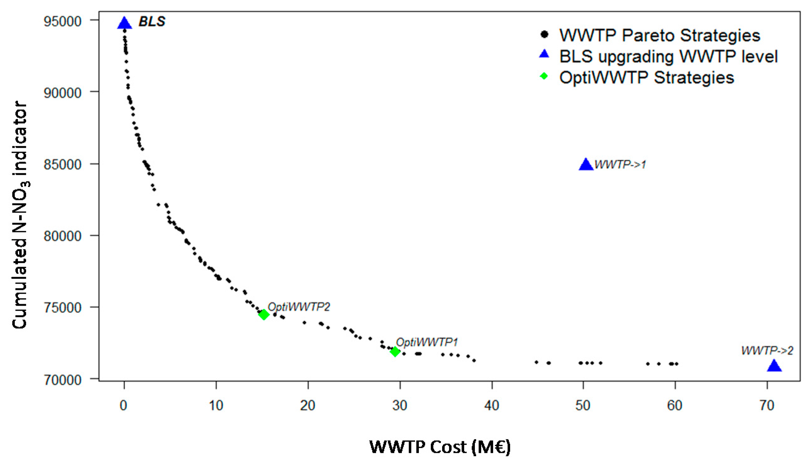
However, management outcomes could be substantially improved by applying the multi-objective optimization capabilities of the framework. Focusing only on point source pollution, a first optimization process was run for WWTPs upgrading decision process while keeping fertilization at BLS conditions. In this case, each management strategy was coded as a chromosome of length 553 (one per WWTP). Each WWTP had three possible options: 0 (no upgrade), 1 (upgrade to level CN), or 2 (upgrade to level CNDP). The population size was 60, a crossover probability of 0.9, and a mutation probability of 0.1. The optimization process was stopped after 60 generations (3600 evaluations of the model), when the improvement from one generation to the next was negligible (convergence criteria).
Figure 6 shows the WWTPs upgrade Pareto strategies, according to the objectives of minimizing implementation cost and minimizing cumulated N-NO
3 pollution. The OptiWWTP1 strategy (which cost 29.5 M€) could achieve a pollution reduction very similar to upgrading all WWTPs to CNDP level (SmartWWTP, which would costs 71 M€). Moreover, investing only 15.2 M€ (OptiWWTP2 strategy) could achieve a pollution reduction of 21.5%, which is not so far to the 26% reduction achievable by upgrading all WWTPs to CNDP level (SmartWWTP;
Figure 5 and
Figure 6;
Table 6). Both OptiWWTP1 and OptiWWTP2 strategies offer a good compromise between economic and environmental objectives. In the OptiWWTP1, 77 plants should be upgraded to CN and 180 to CNDP; in OptiWWTP2 64 plants should be upgraded to CN and 102 to CNDP. No change would occur for the remaining WWTPs.
The multi-objective optimization can also be carried out for mineral fertilization while maintaining WWTPs at the BLS status. In this case the variables considered were the HRU mineral fertilization rates, so the length of the chromosome was 291 (one variable per fertilized HRU). The fertilization rate variables were continuous, ranging from 0 kg/ha to a maximum equal to the double of the HRU mineral fertilizer applied in the BLS scenario. The population size was 50, the maximum number of evaluations 3000 (60 generations), crossover probability 0.9, and mutation probability of 0.1.
The optimization process found fertilization management strategies that were more efficient than the SmartFert strategy for both reducing pollution and increasing the total net income.
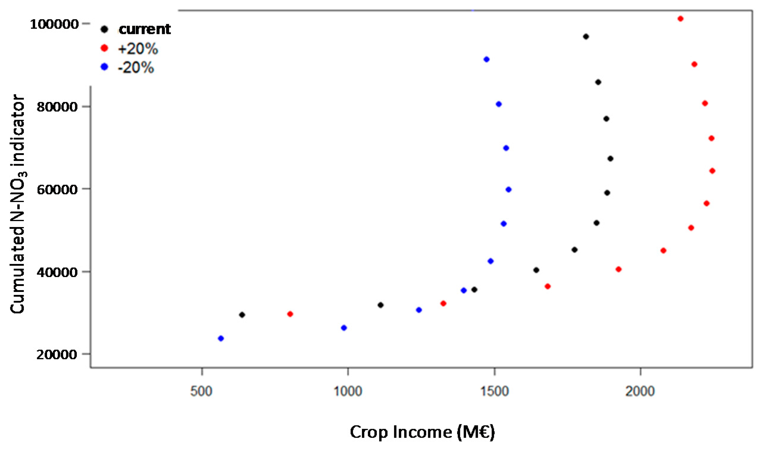
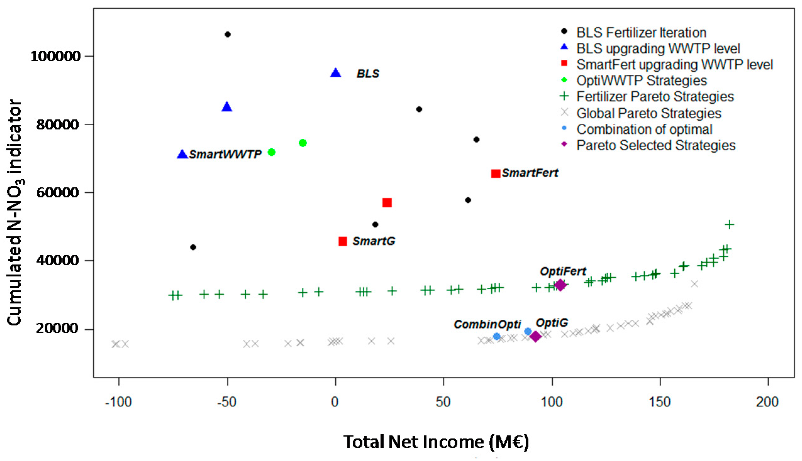
Figure 7 shows the trade-off strategies (green “+”). The Pareto front is slightly sloped, which indicates that it is possible (up to a limit) to improve profitability without significantly increasing pollution if adequate local fertilization rates are applied across the region. Among many, we selected one strategy from the Pareto set, labeled OptiFert in
Figure 7 and
Table 6. This fertilization strategy provides a total net income increase of 100 M€ and a 65% reduction in the N-NO
3 pollution compared to BLS. Compared to SmartFert scenario, it afforded a 50% reduction of pollution.
Finally, a multi-objective optimization run was also performed considering simultaneously all decision variables. In this case, the chromosome length was 824 (291 fertilizations + 533 WWTP). The optimization process was performed with a population size of 80 chromosomes during 50 generations (4000 evaluations), crossover was 0.9, and mutation 0.1. The trade-off strategies (Pareto front) of this run are also shown in
Figure 7 (gray “x”). Significant improvements in the total net income with little increase in the N-NO
3 metric were further identified. Among this last Pareto set, we selected one strategy, labeled as OptiG. This strategy could achieve N-NO
3 reductions of 81% of BLS and 61% of SmartG strategies, with a total net income of 92 M€ higher than the BLS (
Table 6 and
Figure 7).
Two additional strategies were generated by combining the OptiWWTP1 and OptiWWTP2 with the OptiFert strategy selected from the fertilization only Pareto set (
Figure 7). We labeled these as CombinOpti1 and CombinOpti2 in
Table 6 (blue points in
Figure 7). Both strategies yield similar results than OptiG strategy. However, management practices applied in the CombinOpti strategies and in the OptiG are considerably different, especially in terms of WWTP management. In CombinOpti2 102 plants should be upgraded to CNDP level, whereas in OptiG 362 should be upgraded to CNDP level. The implementation cost would raise from 15.2 M€ in CombinOpti2 to 48 M€ in OptiG. However, this higher purification investment in OptiG would be offset by the higher crop revenue achieved by slightly increasing fertilization (and N-NO
3 pollution generated by agriculture). Similarly, the CombinOpti2 and OptiG strategies are very close in terms of objectives (
Figure 7), but are very different in terms of type and spatial distribution of BMPs that are identified. Hence, the global optimum finds synergies between all types of management alternatives; this example shows the advantage of combining considerations for PS and NPS management at once.
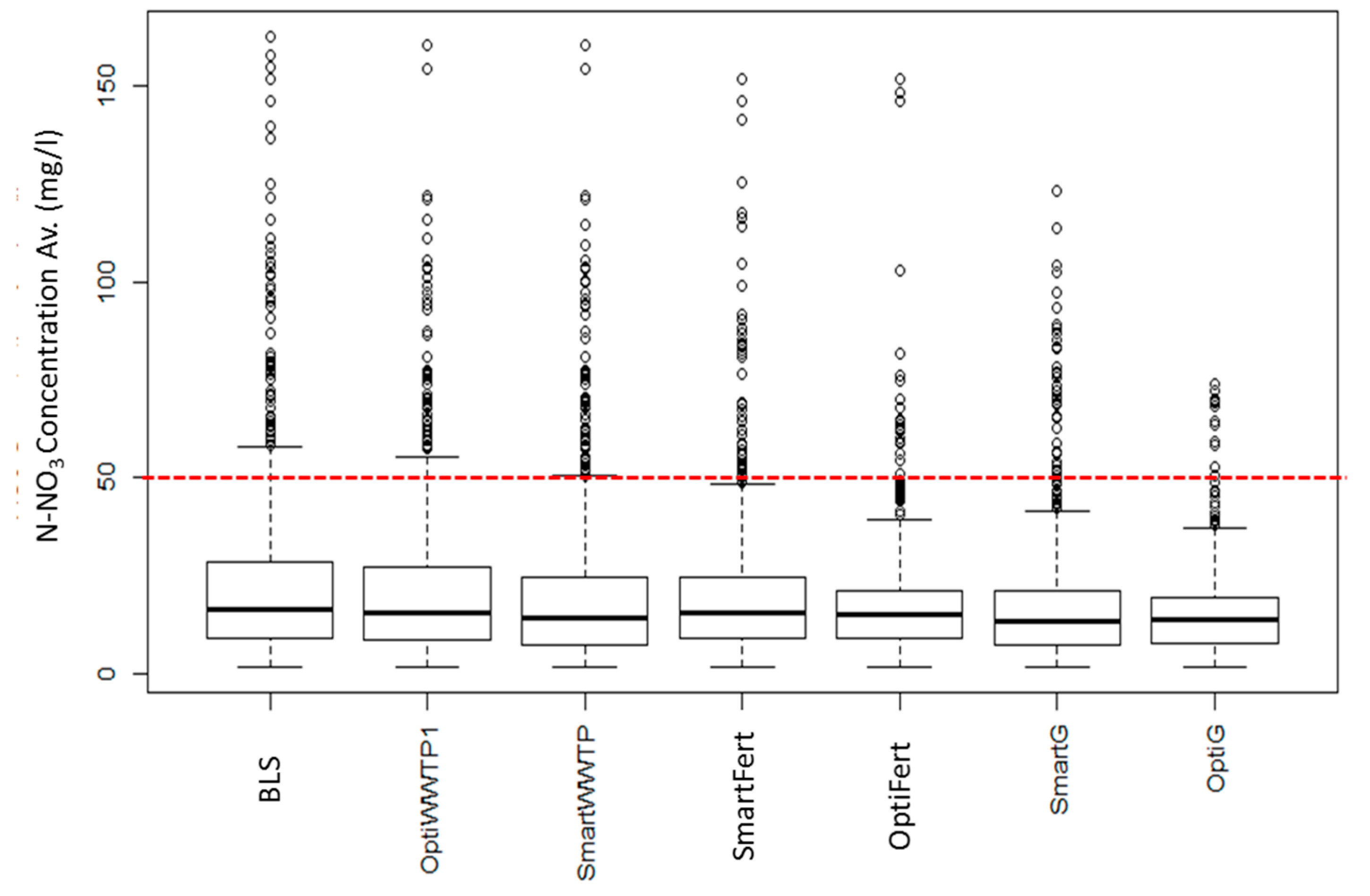
SmartFert and SmartWWTP strategies, respectively, reduce fertilizer use or upgrade WWTPs without considering differences in current pollutant concentration status across the reaches. They are quite efficient in decreasing the average N-NO
3 concentration by almost 6 mg/L (see column labeled “Equation (1)” in
Table 6). They would also reduce the number of reaches with average N-NO
3 concentration exceeding the 50 mg/L by 50% (
Table 6). However, these strategies do not provide total net income and do not reduce the high average N-NO
3 concentrations in the remaining 50% of polluted reaches (
Table 6,
Figure 8 and
Figure 9).
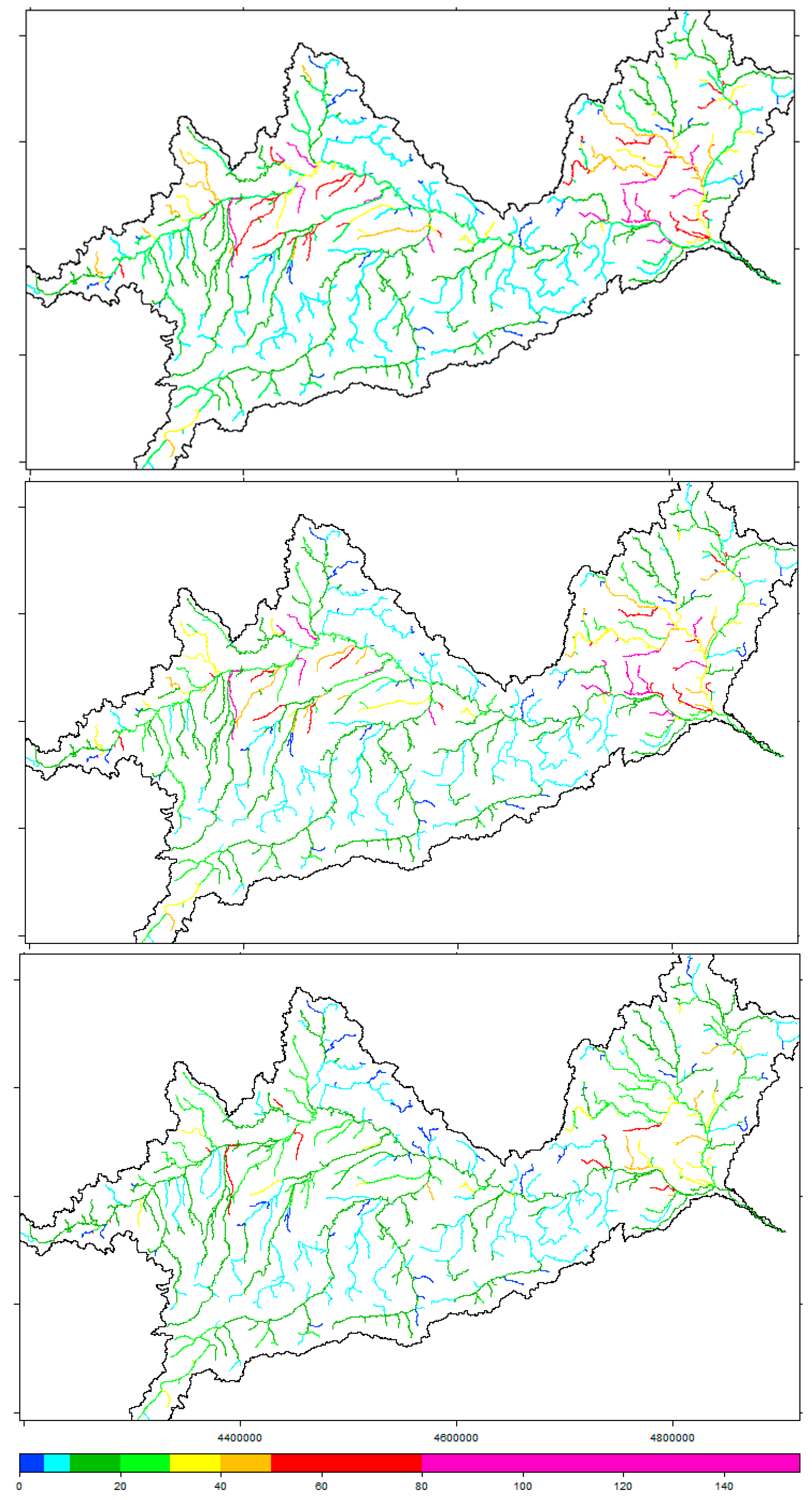
Conversely, management strategies found by applying the optimization routine (such as OptiG) do consider the location where management is applied. The spatial distribution of monthly average N-NO
3 concentration in the reaches of the Upper Danube Basin is shown in
Figure 9 for three different management strategies: BLS, SmarFert and OptiG. Where average N-NO
3 pollution is low (i.e., below the WFD threshold of 50 mg/L) in the BLS, there are no significant differences between the three strategies. Conversely, in the reaches where N-NO
3 concentration threshold (50 mg/L) is exceeded, the improvements are important, especially in the OptiG. The number of reaches where on average the threshold is violated is reduced from 78 to 12. OptiG is the only strategy that could reduce the average N-NO
3 concentration of all polluted reaches to less than 70 mg/L (
Table 6 column labeled as (2),
Figure 8).
Table 6 shows the value of several environmental and economic indicators for each of the strategies described above, in which only two objectives have been considered simultaneously: minimizing the cumulated N-NO
3 metric (Equation (2)) and maximizing the total net income. In a comprehensive decision-making process, the framework could be applied considering simultaneously more than two objectives, for example to account for other pollutants (like PO
3, NH
4, or sediments) or other metrics (Equations (1) and (3); or other economic valuation). In these cases, the analysis would be enlarged to a higher number of dimensions (the Pareto set will be a surface instead of one curve).
Biophysical and economic model results are subject to uncertainties. A correct calibration of the biophysical model and a correct estimate of biophysical and economic parameters are essential to minimize the influence of the uncertainties on the decision making process. Simulations and optimizations performed with R-SWAT-DM allow better understanding of the behavior of the model under different situations.
In addition, the framework allows simple parameter sensitivity analyses to assess which parameters impact the process under study.
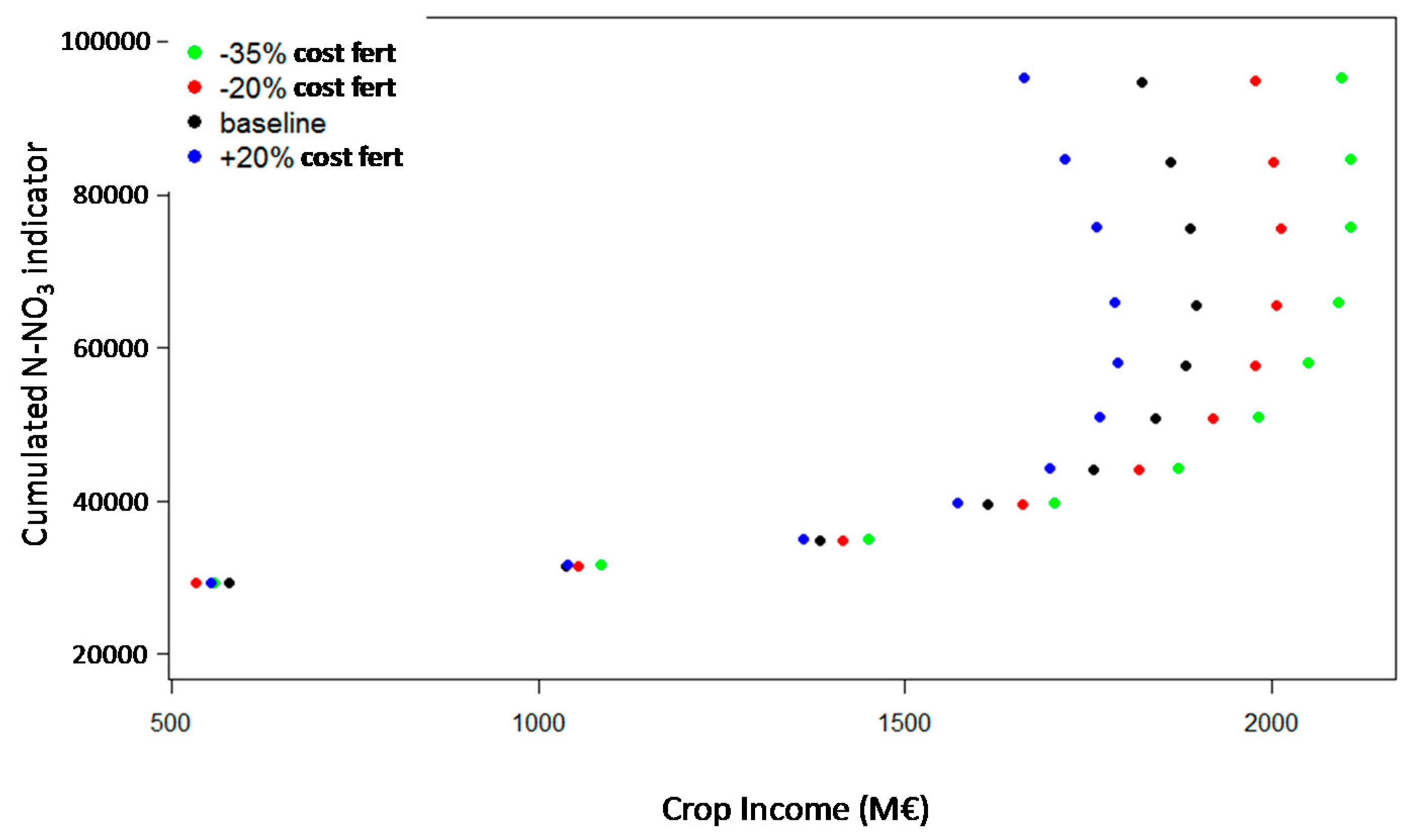
Figure 10 and
Figure 11 show two parameter sensitivity analyses performed by means of the iterative simulation option.
Figure 10 shows the effect of variation in the fertilizer price and
Figure 11 shows the effect of the harvest index coefficient (a SWAT crop parameter that defines the fraction of the total crop biomass removed with the harvest operation) on the final results. As it can be seen, changes in the fertilizer price result in changes of the response curve shape (
Figure 10), whereas changes in the harvest index coefficient shifts the Pareto fronts to the right or to the left (i.e., the income estimation is sensitive to these parameters) but do not change curve shape (
Figure 11). In both cases, however, the strategy benefits in terms of N-NO
3 pollution remain similar.
5. Summary and Conclusions
Although in recent years the Water Framework Directive and the Nitrates Directive have succeeded in achieving some improvement in the nutrient status of many European water bodies, aquatic ecosystems in Europe are still at risk of eutrophication from excessive Nitrogen availability. These risks can be significantly reduced by applying selected BMP efficiently.
An integral simulation-optimization framework (R-SWAT-DM) for optimal allocation of PS and NPS conservation practices was applied to the Upper Danube Basin. The framework uses the spatially distributed watershed model SWAT to assess nonpoint and point source pollution and crop yields under current conditions (baseline) as well as under alternative management scenarios. Management strategies included crop fertilization plans to reduce diffuse pollution and wastewater treatment plant technology upgrading to reduce PS pollution. The economic module allows evaluating the economic benefit or cost associated to each management strategy, accounting for farmers’ gross margins and WWTP upgrading investment cost.
For this application in the Upper Danube Basin, we focused on one environmental objective (i.e., minimizing average monthly N-NO
3 concentration exceeding a 50 mg/L threshold) and on one synthetic economic objective (i.e., maximizing the total net income). Efficient strategies that could significantly improve current water quality status were found. Our analysis suggests that a proper management of mineral fertilization can lead to important environmental benefit without affecting farmer economic income. Reducing the mineral fertilization rate by around 35% will allow obtaining a 30% reduction of N-NO
3 concentration in the most polluted river reaches, while concurrently increasing the total net income by 75 M€. These results are in line with the outcomes of the EUROSTAT analysis of statistics and agri-environmental indicators of the four Upper Danube Basin main Countries. In this region the high input of organic Nitrogen from manure allows indeed to reduce mineral inputs with limited negative effect on crop yields (assuming a correct management of manure is put in place). In this context, for many crops additional mineral fertilizer inputs would result in slight increases of yields that would not be sufficient to repay the extra fertilization cost or the extra environmental pollution. Over-fertilization is a well-known issue in the Upper Danube, and more generally in all of the Danube River Basin [
62]. The fact that farmers may reduce N use and increase their profit is puzzling: a rational farmer should have decided to reduce N use. One explanation could be the lack of information of farmers with respect to best management practices. It could be that local extension services focus more on increasing crop yields than on giving advices to farmers on how to apply N in an efficient way. One policy recommendation could be then to write and disseminate guidelines on best management practices to farmers. Another policy option could then be to propose farmers some insurance mechanisms to secure their crop yield against the perceived loss in income due to reduced fertilization [
63] or to redistribute parts of the gains coming from N reduction strategies to the farmers having voluntary opted to implement actions in the form of subsidies.
Similar reductions in N-NO
3 pollution (measured with the cumulative N-NO
3 metric) could be achieved by upgrading WWTP treatments. The cost of water quality improvements could be relatively low (15 M€) if associated to a spatially efficient choice of the WWTPs to be upgraded. The necessity to upgrade WWTPs was recommended by the European Court of Auditors [
64] as an effective means to abate urban pollution. Since WWTPs are usually owned by municipalities, a massive program of upgrades raises the issue of funding these investments. One part of the investment cost could be passed through final users but local governments, sometimes for political reasons, may be reluctant to strongly increase water and wastewater prices. Another solution is then to activate the European Regional Development Fund and the Cohesion Fund which are available to Member States in particular for co-financing investments, in particular on UWWTPs upgrade and modernization. In the Danube River Basin, an analysis on 28 projects revealed that the EU co-funding has represented on average 62.5% of total expenditures with a minimum of 34% and a maximum of 75% [
65]. These figures suggest that a significant part of the upgrading cost could be covers through EU co-funding is case a municipality goes for a secondary or a tertiary treatment of waste water.
Our study also found that efficient strategies focused on most polluted reaches, whereas water quality was not much improved where N-NO3 concentrations were already below the threshold of 50 mg/L: in these reaches the upgrade of upstream WWTPs even if combined with the reduction of mineral fertilization in the contributing HRUs did not bring about significant improvements. On the contrary, in most polluted reaches, where the N-NO3 concentration exceeds the WFD threshold, significant improvements could be achieved through the combined application of the proposed measures. Thus, by effectively exploiting synergies between PS and NPS best management practices, the number of reaches with excessive N-NO3 concentrations can be reduced from 78 to 12, even with a positive net income (92 M€). However, in some reaches where N-NO3 concentration was most problematic, no combination of the selected measures could reduce N-NO3 pollution to less than the WFD water quality threshold of 50 mg/L. For these reaches, other strategies, such as reduction of livestock density, different crop rotations, land use changes, irrigation practices, should be contemplated in addition to those considered herein.
The formulation of conservation strategies is under the responsibility of transboundary river basin organizations (such as the International Commission for the Protection of the Danube River for Danube River Basin) but these organizations need scientific evidence and tools to measure the impact and effectiveness of proposed plans. The decision support system does not guarantee the implementation of the optimal solutions, but it provides the data, results and scenarios that feed into political negotiations on the development of sustainable strategies. If some strategies are not considered feasible or acceptable further constraints may be added in the tool to identify new optimal solutions.


 ,
, 


