Source Apportionment of Annual Water Pollution Loads in River Basins by Remote-Sensed Land Cover Classification

Abstract

In this study, in order to determine the efficiency of estimating annual water pollution loads from remote-sensed land cover classification and ground-observed hydrological data, an empirical model was investigated. Remote sensing data imagery from National Oceanic and Atmospheric Administration (NOAA) Advanced Very High Resolution Radiometer were applied to an 11 year (1994–2004) water quality dataset for 30 different rivers in Japan. Six water quality indicators—total nitrogen (TN), total phosphorus (TP), biochemical oxygen demand (BOD), chemical oxygen demand (COD), and dissolved oxygen (DO)—were examined by using the observed river water quality data and generated land cover map. The TN, TP, BOD, COD, and DO loads were estimated for the 30 river basins using the empirical model. Calibration (1994–1999) and validation (2000–2004) results showed that the proposed simulation technique was useful for predicting water pollution loads in the river basins. We found that vegetation land cover had a larger impact on TP export into all rivers. Urban areas had a very small impact on DO export into rivers, but a relatively large impact on BOD and TN export. The results indicate that the application of land cover data generated from the remote-sensed imagery could give a useful interpretation about the river water quality.

1. Introduction

Changing land use and land management practices are regarded as amongst the most important factors that can alter hydrological systems and water quality, which have become increasingly important to catchment stakeholders, such as management groups, land owners and government departments [1,2,3,4]. Generally, a river’s water quality is linked to the land cover in the watershed and is degraded by changes in the land cover patterns on their watersheds as human activities increase [5,6,7,8]. Different studies have increasingly recognized that human action at the landscape scale is a principal threat to the ecological integrity of river ecosystems and water quality [9,10,11,12,13,14,15]. However, the information on the sources of pollutants in catchments and on the response of water quality to changing land use practices is still limited in many catchments [16,17,18,19,20]. It is therefore important to understand the relationships between catchment characteristics and river water chemistry, which provides a base for determining how future changes in land cover and use and climate will impact on river water quality.

In Japan, the water quality of rivers has been improved by legislation on sewage, drainage, etc. However, the water quality cannot be said to have been restored to its natural conditions because the pollution from non-point sources can increase even when factory drainage and domestic drainage are improved by law [21]. Therefore, it is still necessary to take prevention measures to control non-point source pollutants for maintaining the natural ecosystem and environment [22,23]. Among these, identification of the water pollution loads from different sources is important. To this end, statistic methods and hydrological modeling have been proposed and applied to estimate the contribution from different water pollution sources. By using multivariate statistical techniques, Shrestha and Kazama [24] evaluated the temporal/spatial variations in the Fuji river basin, illustrating the usefulness of multivariate statistical techniques for identifying pollution sources/factors and understanding temporal/spatial variation. Duan et al. (2015) developed a SPARROW-based (SPAtially Referenced Regression on Watershed Attributes) watershed model to estimate the sources and transport of suspended sediments in surface waters of the Ishikari River basin [25]. Recently, remote sensing was used to evaluating water quality. Oki and Yasuoka [26] mapped the potential annual total nitrogen load in the river basins of Japan with remotely sensed imagery of 2006. However, the non-point source pollutants are transported to water body is still unclear.

Therefore, in a previous study we have analyzed the relationship between land cover types and potential annual water pollution loads and improved an empirical model to successfully calculate potential annual water pollution loads in 30 river basins in Japan by using the collected dataset in the year of 1996 [27]. Based on these previous results of estimating total water pollution loads in year 1996 for 30 river basins, the objectives of the present study are to (1) test the model prediction capability with long term dataset; (2) modify the original empirical model to account for the water pollution loads from each land cover classification; (3) examine and analyze the capability of this method for apportioning long term potential annual loads of water quality indicators such as total nitrogen (TN), total phosphorus (TP), biochemical oxygen demand (BOD), chemical oxygen demand (COD), and dissolved oxygen (DO) in river basins. The results of this study will be very useful to model the linkage between river water quality and land cover classes by separately considering the impact of each land cover type on the water pollution loads.

2. Materials and Methods

2.1. Collection of Long-Term Dataset

In order to measure and assess changes in vegetation phenology and conditions as well as perform land cover type classification, this study uses 26 National Oceanic and Atmospheric Administration (NOAA) Advanced Very High Resolution Radiometer (AVHRR) images showing maximum annual normalized difference vegetation index (NDVI), at 1.1 km pixel resolution, across Japan for each year between 1984 and 2009. The NOAA AVHRR data was produced by the Sawada and Takeuchi Laboratory, Institute of Industrial Science, University of Tokyo. They were used to produce a land cover distribution map [28]. AVHRR data were geometrically corrected based on ground control point (GCP) matching by using PaNDA software, and registration error over the image was less than 1 pixel. PaNDA is a free software package for NOAA data analysis [29]. The AVHRR NDVI products were also provided by laboratory of Sawada and Takeuchi [28]. The NDVI can be calculated according to the following equation [30]:

$$\text{NDVI}=\frac{({\rho }_{780}-{\rho }_{670})}{({\rho }_{780}+{\rho }_{670})}$$

(1)

where, ${\rho }_{780}$ represents the near infrared band value for a cell, ${\rho }_{670}$ represents the red band value for the cell. Daily NDVI was calculated using Band 1 (0.58–0.68 μm) and Band 2 (0.725–1.10 μm) images to produce the monthly maximum NDVI imagery, and by using the 12 monthly maximum NDVI imagery datasets, the effects of clouds on seasonal land cover changes can be removed to produce each yearly maximum images. All the processing was conducted by using the remote sensing software ERDAS IMAGE (Version 9.2). The Iterative Self-Organizing Data Analysis Technique Algorithm (ISODATA) [31,32], which is an unsupervised classification, was used to produce a yearly land cover classification map of Japan using the 12 monthly maximum NDVI imagery datasets. Figure 1 shows an example of the generated land cover maps in 1996. The river basin map was superimposed on the land cover classification map to calculate the area of land cover types of each river basin. The results were then divided by the river basin area to determine the percentage of the area covered by each type of the land cover.

Table 1. Statistical parameters of land cover (SD means standard deviation; CV means coefficient of variation).

Variables	Mean	Range	SD	CV%	Mean Percent
LU1 (km2)	222.3	4.0–1363.0	299.8	134.8	10.1%
LU2 (km2)	450.2	<0.01–4721.0	1059.7	235.4	20.4%
LU3 (km2)	579.7	<0.01–5365.0	1091.1	188.2	26.2%
LU4 (km2)	646.0	<0.01–2696.0	760.6	117.7	29.2%
LU5 (km2)	311.0	<0.01–1653.0	464.9	149.5	14.1%

Notes: Abbreviations are as follows: LU₁, urban area; LU₂, beech type natural vegetation; LU₃, beech type secondary vegetation; LU₄, Camellia japonica community; LU₅, plantation and field weed community.

shows some characteristics of the land cover classes, suggesting that Camellia japonica community (LU₄) was the largest land cover, occupying about 29.2%, followed by beech type secondary vegetation (LU₃, about 26.2%), beech type natural vegetation (LU₂, about 20.4%), and plantation and field weed community (LU₅, about 14.1%). It can be found from this table that the maximum variation in land cover was observed for beech type natural vegetation (235.4%) and minimum of variation was observed for Ccamellia japonica community (117.7%). For detecting the relationships between pollutant load and basin characteristics, the Pearson correlation [33] was conducted by using MATLAB for the above-collected dataset. As for the pollutant load per area, we did not find a significant correlation coefficient between them and the five land cover classes. Only for beech type natural vegetation were the correlation coefficients of TN, COD, and DO a little bit higher. However, significant correlation coefficients between pollutant loads and land cover were found for land cover of urban area, beech type natural vegetation, and beech type secondary vegetation. The urban area is highly related to the export of TN, TP, BOD, COD, and DO from river basins.

As for the hydrochemical datasets, we collected available long-term observation data of river discharge, TN, TP, BOD, COD, and DO concentration for 30 selected river outlets (Figure 2), which represented different regions of Japan, for 11 years (1994–2004). Statistical analysis has been conducted for the collected monthly hydrochemical database from the National Land with Water Information (http://www1.river.go.jp/) monitoring network [14].

Table 2. Statistical parameters of the studied water quality variables (SD means standard deviation; CV means coefficient of variation).

Variables	Mean	Range	SD	CV%
TN (mg/L)	1.7	0.5–11.3	2.2	129.7
TP (mg/L)	0.1	<0.01–0.8	0.2	162.6
BOD (mg/L)	1.8	0.2–14.2	2.5	137.9
COD (mg/L)	2.9	0.8–9.5	1.9	63.5
DO (mg/L)	10.1	6.7–11.7	1.0	10.3

shows the statistical description of the collected water quality data. For all 30 sites over Japan, large variations of annual concentration of TN, TP, and BOD were observed between rivers, with a smallest coefficient of variation as 10.3% for DO and highest value as 162.6% for TP [14]. The large spatial variation of TP concentration are corresponding to the large differences in regional characteristics including population, topography, geology, agricultural activities, and land use in 30 river basins. Furthermore, significant correlation coefficients from the Pearson correlation analysis [32] for detecting the relationships between water pollutant loads and land cover have been found [14].

For a clearer understanding of the spatial distribution of water pollution loads in Japan, the basin area and river mouth discharge for each catchment are listed in

Table 3. Basin area and river mouth discharge for each catchment.

Catchment	1	2	3	4	5	6	7	8	9	10
Area (km2)	1078	10,617	2252	4198	4594	1189	6869	858	1539	1217
Q (m3/L)	3.1	163.2	56.6	186.8	235.0	60.6	367.7	86.3	9.3	11.6
Catchment	11	12	13	14	15	16	17	18	19	20
Area (km2)	237	3878	582	1277	4854	4762	3695	2069	831	361
Q (m3/L)	3.2	40.4	6.4	34.7	132.6	205.3	80.4	40.2	4.2	6.8
Catchment	21	22	23	24	25	26	27	28	29	30
Area (km2)	511	929	1202	557	650	1368	509	2164	510	922
Q (m3/L)	14.1	18.6	45.1	18.5	17.9	36.7	11.3	47.0	19.3	24.2

. The catchment areas which have an area larger than 2000 km² are highlighted with shaded color. We found that catchments 2, 3, 4, 5, 7, 12, 15, 16, 17, 18, and 28 are relatively large compared to others and also have large total river discharge volumes, both of which contribute to large total water pollution loads.

Among the collected hydrochemical datasets, the data from 1994 to 1999 (6 years) were used for model calibration. The remaining 5 years of data (2000–2004) were used for model validation. Annual water pollution load in rivers was estimated as the product of the annual average water quality concentration and the annual discharge at the outlet of each river. All the original water quality and river discharge data were measured by the National Land with Water Information (http://www1.river.go.jp/) monitoring network.

2.2. Estimating Water Poolution Loads from Different Land Cover Classifications by a Modified Empirical Model

An empirical model based on the above data was used to simulate annual pollutant loads by linking load with different anthropogenic and natural variables [14,26]. To estimate annual pollutant loads from each land cover classification for each river basin, this model was modified in this study. The water pollution load exported from each river basin i can be presented as follows:

$$\frac{L_i}{A_i}=\mathrm{k}·{(\frac{Q_i}{A_i})}^n·(\frac{S_i}{A_i})$$

(2)

where L_i (kg/year) is the total annual water pollution load exported from river basin i, which can be calculated as the product of average water quality concentration and river discharge. A_i (km²) is the area of river basin i, Q_i (m³/year) is the annual river discharge at the river outlet of river basin i, S_i (kg/year) is the annual runoff load accumulated from different land covers in river basin i; k and n are empirical coefficients which are calibrated value by using optimization method or trial and error method. In this equation, the effect of basin area on water pollution load is removed with the division by basin area.

The annual water pollution load accumulating in river basin i, i.e., S_i, is expressed by:

$$S_i={\displaystyle \sum }_j^5(L{U}_j·\acute{A_{ij}})$$

(3)

where j (values 1–5) means each land use category of class 1 to class 5 shown in Figure 1. LU_j (kg/km²·year) is the coefficient named as runoff load factor of each category j, and $\acute{A_{ij}}$ (km²) is the land cover area of each category j in river basin i. Here, LU_j (kg/km²·year) represents the average value of the annual total water pollution loads accumulating in each category j in all of Japan.

As shown in the above Equation (2), there are several parameters which should be estimated using the collected hydrochemical and land cover dataset. In this study, the simplex method (also known as the polytope method), which linearly adjusts model parameters to meet convergence criteria [34,35], was used to estimate k, n, and LU_j (j = 1 to 5).

3. Results

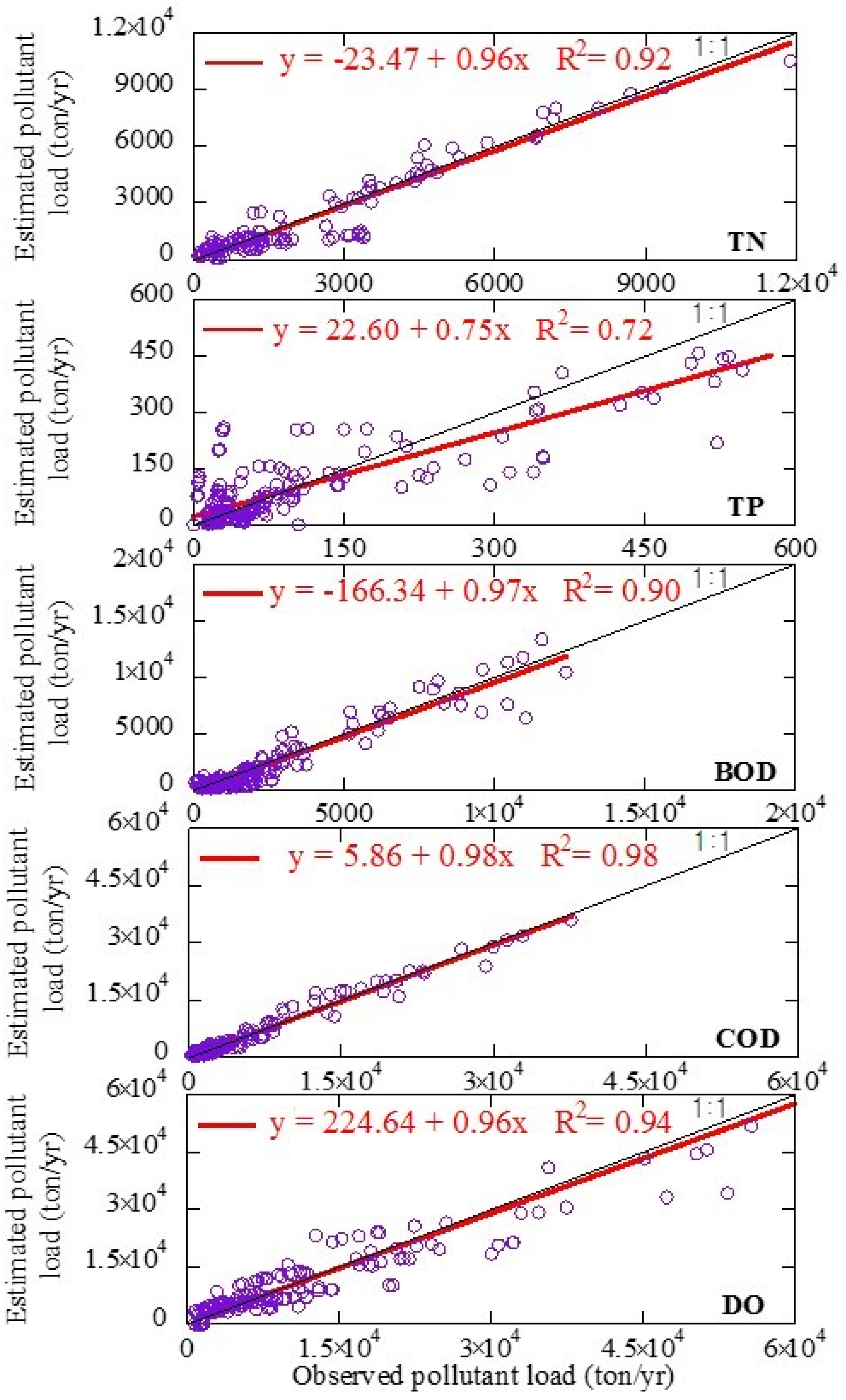
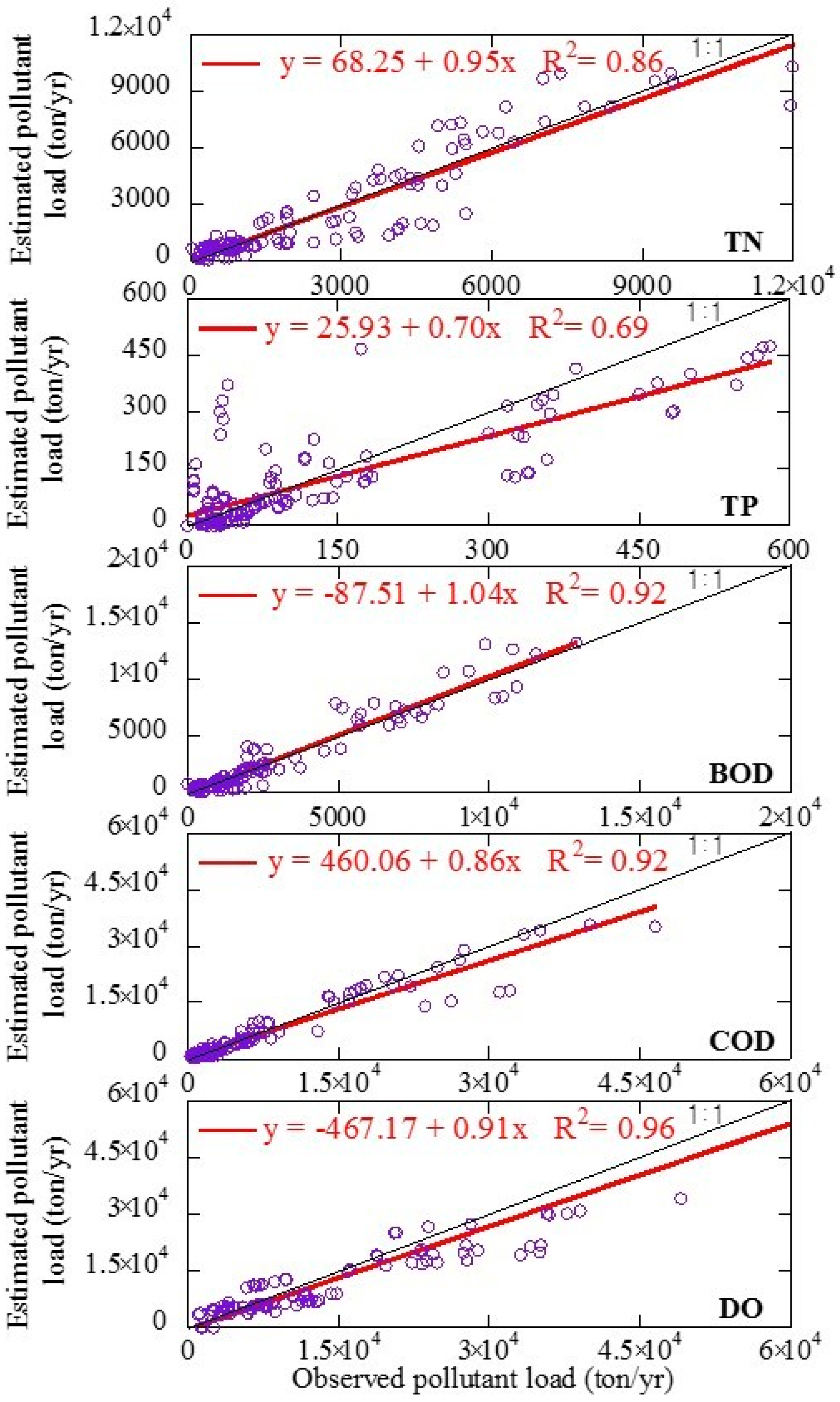
3.1. Model Calibration (1994–1999) and Validation (2000–2004)

We estimated annual discharged water pollution loads using the data from 1994 to 1999 for the 30 study basins. The observed and predicted water pollution loads were compared in the 30 river basins for the calibration period (1994–1999). The regression of predicted versus observed water pollution loads resulted in high correlation coefficients: R² = 0.92, 0.72, 0.90, 0.98, and 0.94 for TN, TP, BOD, COD, and DO, respectively, indicating that water pollution loads estimates had sufficient reproducibility for the calibration period (Figure 3). Furthermore, we can see from

Table 4. Estimated values of model parameters.

Parameter	k	n	LU1	LU2	LU3	LU4	LU5
TN	0.09	0.81	0.80	0.04	0.09	0.00	0.34
TP	0.17	0.44	0.36	0.83	0.91	0.52	0.76
BOD	0.14	0.73	0.68	0.29	0.32	0.15	0.28
COD	0.19	0.70	1.50	0.97	0.76	0.55	0.50
DO	1.62	0.34	0.00	115.73	33.40	47.92	71.08

that the calibrated river discharge factor, i.e., coefficient n in Equation (1), has the smallest value for DO and largest for TN, and has almost the same value for BOD, COD, and TP.

Figure 3 and Figure 4 show the model calibration and validation results with the comparison of the measured and validated annual water pollution loads. The magnitude of the predicted annual water pollution loads closely followed the measured data in most of the studied rivers. We found good simulation results for TN, BOD, COD, and DO when comparing the figures with the calibration results. The simulation of TP showed the smallest correlation coefficient between the observed and modeled TP load. In terms of the description itself, it appears that the model overestimates TP loads from some basins in which the actual TP is very low.

The above calibration and validation were conducted at the whole-of-catchment scale, which includes all the land cover types. To evaluate the accuracy of the predictions at the scale of individual land cover types, the water pollution loads were predicted from different land cover type.

Table 5. Accuracy of the predictions at the scale of individual land cover types.

	LU1	LU2	LU3	LU4	LU5
TN	0.71	0.35	0.33	0.00	0.00
TP	0.43	0.34	0.44	0.00	0.00
BOD	0.74	0.66	0.60	0.00	0.00
COD	0.83	0.78	0.66	0.00	0.00
DO	0.79	0.72	0.68	0.00	0.00

shows the R² coefficients for predicting TN, TP, BOD, COD, and DO by using each land cover type. From this table, it can be found that the most accurate prediction of water pollution loads is that predicted by using land cover of urban area. The second accurate prediction of water pollution loads is that predicted by using land cover of beech type natural vegetation. The least accurate predictions of water pollution loads are those predicted by land cover of Camellia japonica community, and Plantation (Cryptomeria japonica and Cryptomeria) and field weed community.

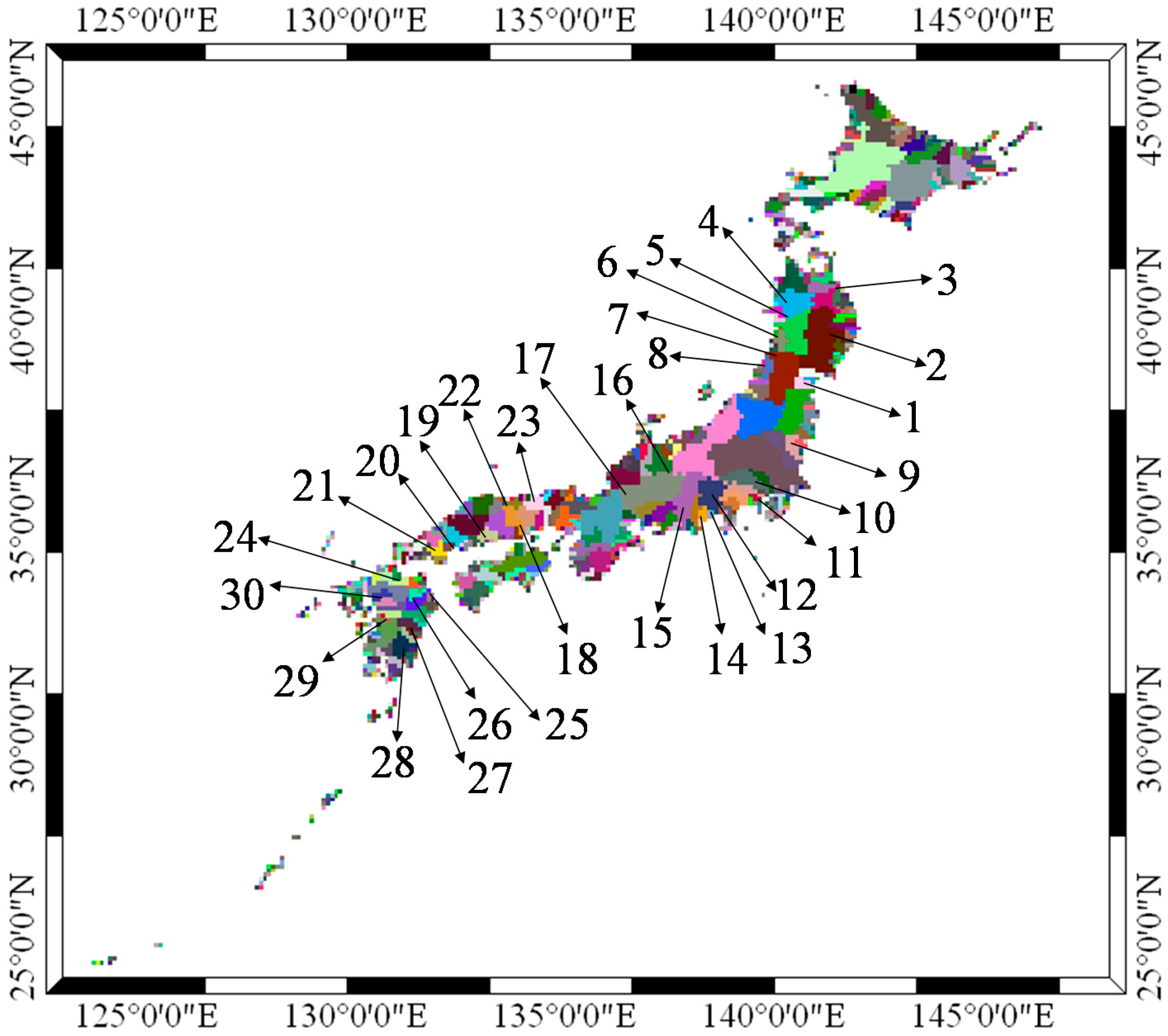
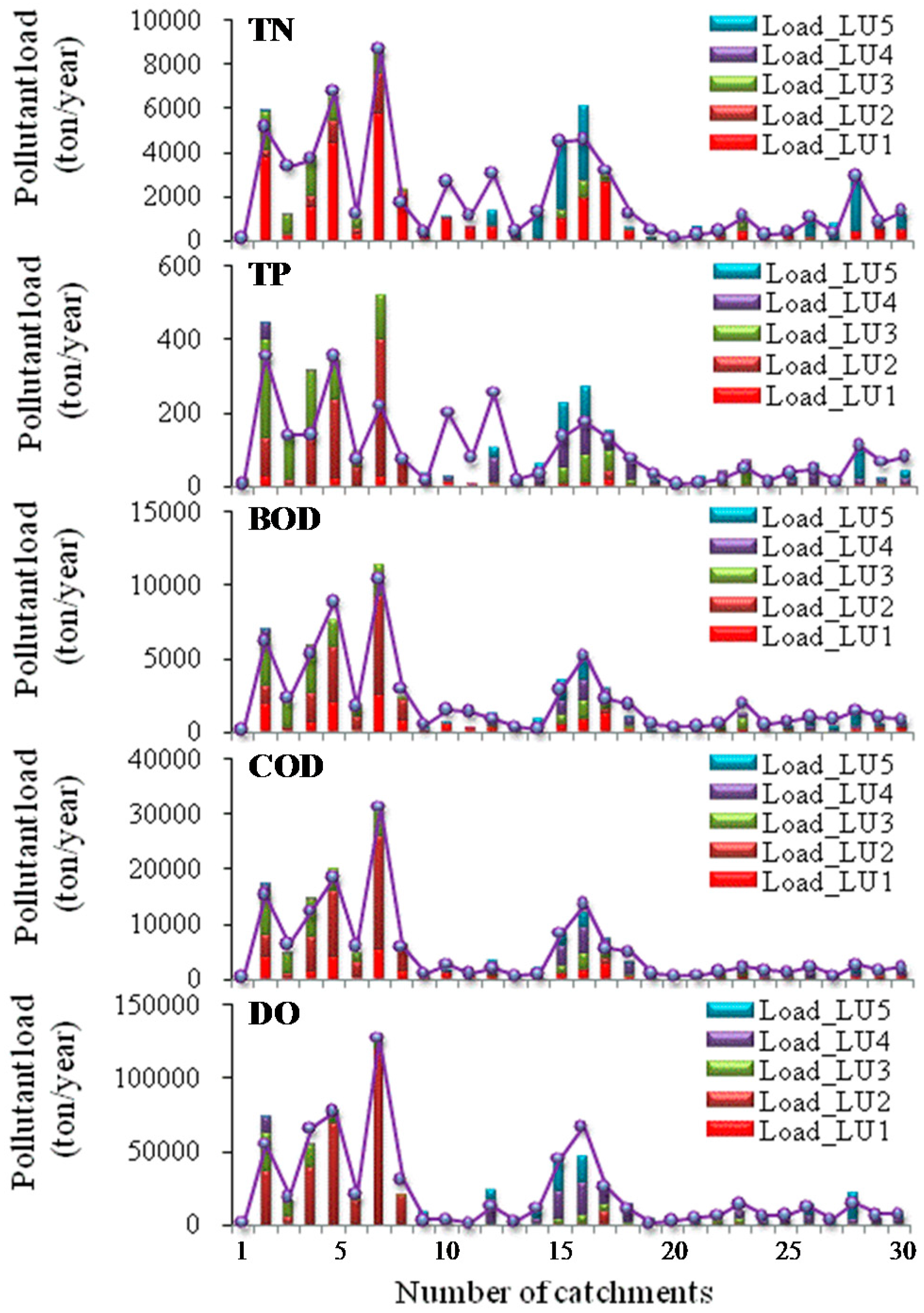
3.2. Spatial Comparison of Water Pollution Loads in the 30 Rivers

Considering the water pollution loads of 1996 from our previous study [24], Figure 5 shows the water pollution loads associated with different land cover classifications in the 30 catchments for 1996, as an example. There was good agreement between the observed and modeled water pollution loads for TN and COD. For most of the catchments, the results are good at simulating water pollution loads for BOD and DO. As for TP, there are differences between the observed and modeled load. Moreover, it can be found from the figure that urban areas mainly impacted TN, BOD, and COD loads. The effect of urban areas on TP and DO was very small. Additionally, it is interesting to find that the large water pollution loads of TN, TP, BOD, COD, and DO mostly belong to the river basin in the northern part of Japan, namely Kanto Region (from catchment 1 to 9). The second highest water pollution loads are found in central part of Japan, namely Kansai Region (from catchment 10 to 17). The water pollution loads are mostly very small in the western part of Japan (from catchment 18 to 30). It can be also found that the impact of urban area on water pollution loads is large in both Kanto Region and Kansai Region, in which the economic is well developed and population density is much higher than other parts of Japan.

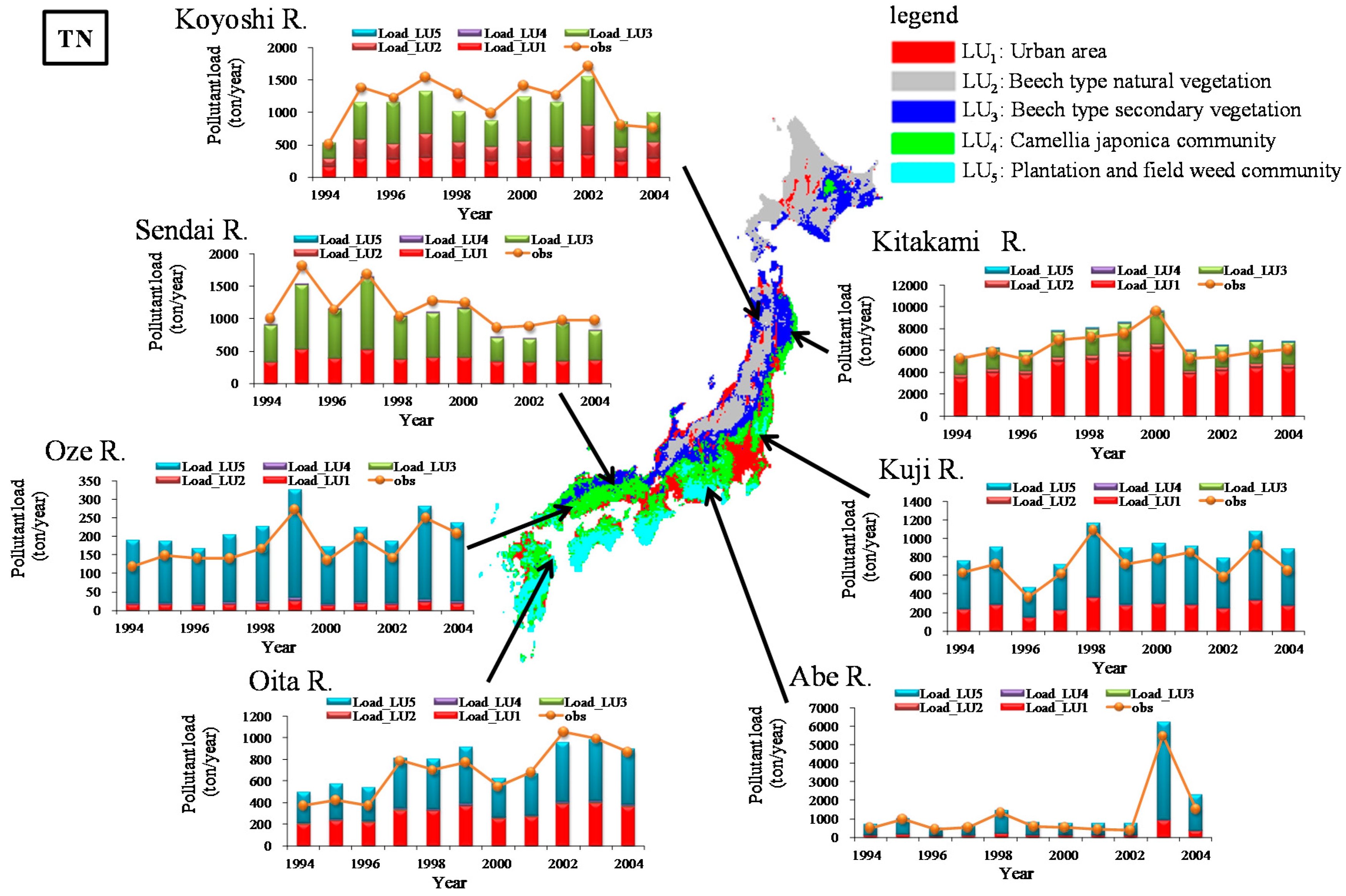
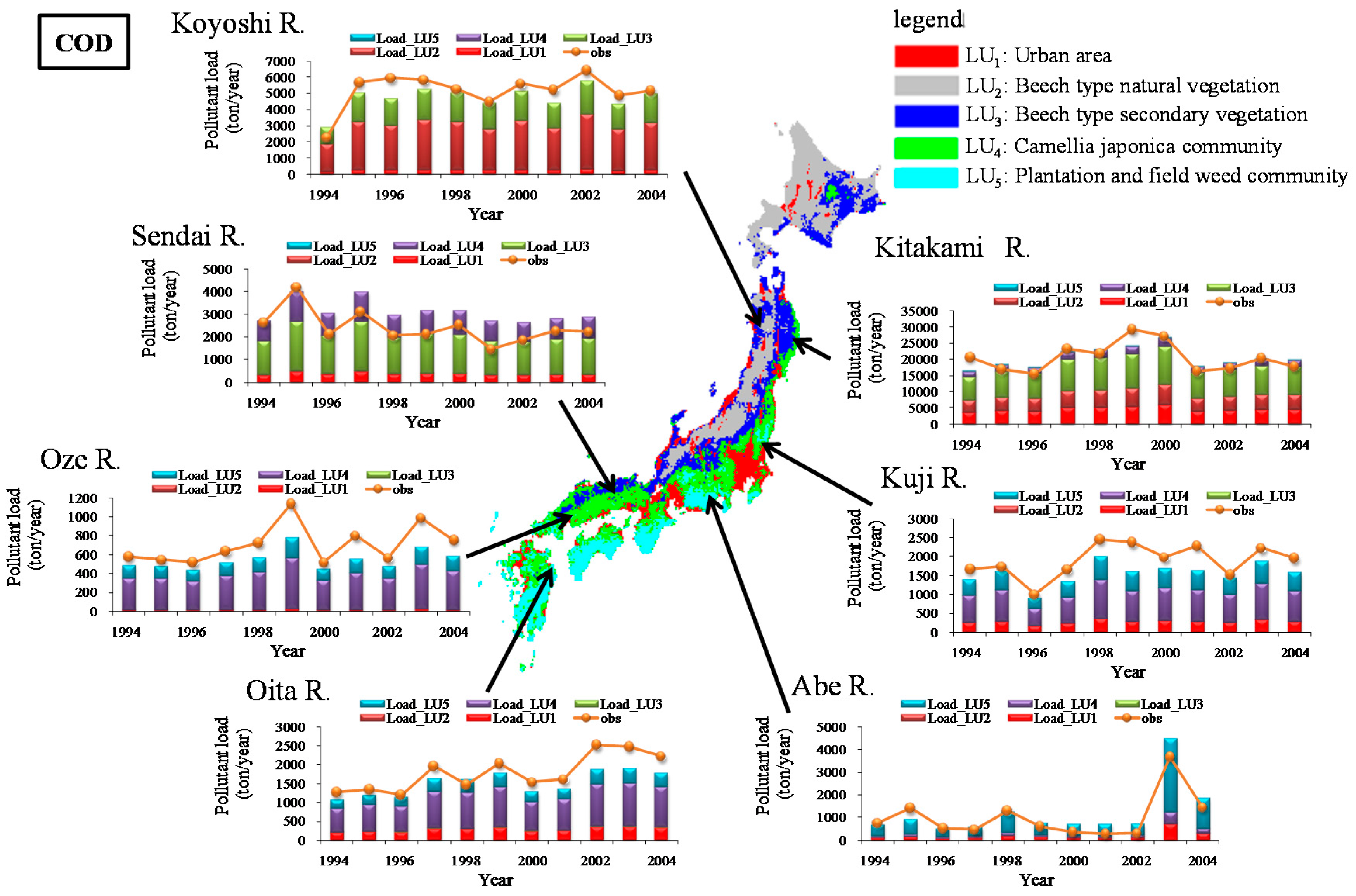
3.3. Long-Term Variation in Water Pollution Loads Estimated from Different Sources

As evident from the calibration and validation results, the model exhibited a good association between measured and predicted water pollution load values. Based on the above simulation, seven river catchments including Koyoshi, Sendai, Oze, Oita, Kitakami, Kuji, and Abe, which are representative of the 3 main regions (north, central, and western), were selected to take as the examples to elaborate long-term variation in water pollution loads estimated from different sources from 1994 to 2004. Contributions of different sources to major water quality variables can be then identified for the investigated river basins. Figure 6 and Figure 7 show examples of TN and COD for seven typical rivers for which long-term observation data were available. The yellow line represents the observed water pollution loads. The vertical bars indicate the water pollution loads from different land covers. From Figure 6, it can be found that urban areas had a large impact on TN export into rivers. It is probably because there are many nitrogen sources such as residential fertilizers, septic systems, and domestic animal waste in urban areas. Even though the urban area ratios were low for the Kitakami, Kuji, Oita, Sendai, and Koyoshi Rivers, the water pollution load from urban areas was still very high. Therefore, beech type secondary vegetation (LU₃) and plantation field weed community (LU₅) contributed strongly to the TN loads in the rivers, whereas beech type natural vegetation (LU₂) made a small contribution. Discharge from the Abe River increased dramatically in 2003, from 10 m³/s to 146 m³/s, and TN export increased accordingly. It also can be found that a small contribution of TN might make a large difference to riverine TN in small catchments.

From Figure 7, it can be found that urban areas also had a high impact on COD export into rivers. As with the COD results, the pollutant load from urban areas (LU₁) was high for the Kitakami, Kuji, Oita, and Sendai Rivers. Land cover of beech type secondary vegetation (LU₃) and Camellia japonica community (LU₄) had a large effect on COD export into rivers. The impact from land cover beech type natural vegetation (LU₂) was small, except for its effect on the Koyoshi River. As mentioned above, discharge from the Abe River increased suddenly in 2003, and COD export increased accordingly.

The same analysis was conducted for the other water pollutant indicators. We found that beech type natural vegetation (LU₂) and beech type secondary vegetation (LU₃) had a larger impact on TP export into all rivers. Urban areas (LU₁) had a very small impact on DO export into rivers, but a relatively large impact on BOD export.

4. Discussion

4.1. Model Advantage Compared with Conventional Method

As stated in the above, Figure 3 and Figure 4 showed good agreement between modeled and measured water pollution loads for the calibration and validation periods. In the calibration phase, attempts were made to minimize the root mean square error and obtain R² values closest to a value of unity. However, except for the BOD validation period, the model underestimated pollutant fluxes. This may be partly due to the model’s inability to capture the effects of consecutive heavy rainfalls that caused floods throughout Japan. A statistical evaluation of the measured and observed water pollution loads yielded high R² values close to 1.0, with a high slope close to 1.0 for all pollution indicators, except TP. Therefore, using this method, it was possible to estimate the annual total water pollution load discharged from the river basins in Japan and identify water pollution load changes compared with conventional methods that estimate annual total water pollution loads based on the sum of a basic unit, which is the discharge rate of total pollutant load to each land cover category in a basin. Determining a basic unit for each land cover category is difficult, because there are many databases supplying basic units of total pollutant loads evaluated in various river basins, gained by different methods, and covering different sites and seasons. Compared with the conventional method (such as water quality basic unit method), it was easier to assess annual pollutant loads in river basins using the model proposed in this study.

4.2. Problems of Water Pollution Loads

Since Figure 3 and Figure 4 are the results of multiple years of different basins, land cover in those basins for different years is changing. The precipitation and TP leaching may rates may have differed from the rates at which the models were calibrated. Another reason may be that diffuse phosphorus source pollution is associated with agriculture because of the potential movement of fertilizers from the land surface directly into rivers and streams or through permeable soil to groundwater. For example, Camellia japonica community should be fertilized in late winter or very early in the spring when new growth begins, using a slow-release. The main mechanism of phosphorus loss from agricultural soil is through erosion, while leaching to groundwater and phosphorus loss due to landslide and debris flow cannot be considered in this method. Therefore, the effects of landscape management and of specific pollution practices on TP were difficult to define or quantify in the current study. Figure 6 and Figure 7 give us a brief image of the trend of water pollution loads and indicate that in most of the rivers in Japan, water quality management has proven successful in improvement of BOD and COD through stringent discharge regulation, development of sewage systems, etc. However, the risk of water pollution still exists in some rivers. For example, in the Oita River the water pollution loads of both TN and COD are not decreasing, as shown in Figure 6. In some water bodies, the environment status of DO has been worsening rather than improving [36].

4.3. Model Limitation

On the other hand, the approach used in this study has some limitations. The most important limitation is the uncertainty in parameter calibration. The polytope method linearly adjusted model parameters to meet convergence criteria for the estimation of k, n, and LU_j. The parameter values shown in Table 4 may change, however, as characteristics of the river basins change. Additionally, we found that the TN, BOD, and COD runoff load factors from urban areas were higher than those of other land cover types (beech type natural vegetation, beech type secondary vegetation, Camellia japonica community, and plantation field weed community). In another word, these results indicate higher levels of TN, BOD, and COD from urban areas. In urban areas, the nitrogen concentration of rain is higher than for other natural land covers due to various factors such as atmospheric pollution [26]. Moreover, total water pollution loads are discharged from urban areas, unlike in forested areas, where the total water pollution loads cannot be discharged easily due to forest uptake and soil absorption. In addition, the BOD and COD concentrations of urban area river waters were higher than those of other natural land cover areas due to human activities. Furthermore, the results of river discharge factor, i.e., coefficient n in Equation (1), differed slightly from those of He et al. [14], who used the hydrochemical dataset from 1996. In the present study, we used the average of values from 1994 to 2004 for all hydrochemical datasets (river discharge, TN, TP, BOD, COD, and DO). This means the size of the calibration dataset also has impact on the parameter calibration. In addition, n was small, which does not mean that the correlation between DO load and river discharge was weak; rather, the value of the coefficient n was attributable to the magnitude of the data, and BOD load ranged from several hundreds to tens of thousands, and TP load ranged from zero to several hundred.

Furthermore, the parameterized water quality model in this study simplified the complex surface water hydraulics, chemical process, and transport processes. It works on yearly time scale simulation without providing the seasonal change of water quality in rivers and the impact of river discharge on water quality concentration. Therefore, the process-based water quality model can be more useful in case the detailed hydrochemical process needs to be accounted for. In addition, the NOAA–NDVI generated land cover classification map decides the reliability of the water quality model. However, the relationships between NDVI and water quality are likely to change with atmospheric CO₂ concentrations, temperature, precipitation, and so on in the future. This can be more clearly demonstrated in process-based water quality models. Even though there are various limitations with this approach, this study gives a simple and efficient way to source apportionment of annual water pollution loads in river basins by remote-sensed land cover classification.

5. Conclusions

The major objective of this study has been to apply a simple empirical water quality model for examining the water pollution loads from land cover classifications. The authors analyzed the relationship between long-term observation hydrochemical data and land cover classifications estimated from NOAA AVHRR imagery. Statistical analysis revealed large spatial variations in pollutant concentrations of TN, TP, BOD, river discharge, and land use. Urban areas were highly associated with the export of TN, BOD, and COD from river basins. This study indicated that urban and forest land may be the dominant sources of water pollution loads. The simple empirical water quality model was modified and applied successfully in 30 rivers in Japan. Calibration and validation results also indicated that the proposed simulation technique was useful for predicting water pollution loads in the river basins. As a conclusion, this study illustrated the usefulness of using land cover classification and an efficient empirical model for identification of pollution sources and understanding variations in water quality for effective water quality management.

References

1. Changnon, S.A.; Demissie, M. Detection of changes in streamflow and floods resulting from climate fluctuations and land use-drainage changes. Clim. Chang. 1996, 32, 411–421. [Google Scholar] [CrossRef]
2. He, B.; Wang, Y.; Takase, K.; Mouri, G.; Razafindrabe, B.H. Estimating land use impacts on regional scale urban water balance and groundwater recharge. Water Resour. Manag. 2009, 23, 1863–1873. [Google Scholar] [CrossRef]
3. Duan, W.; He, B.; Nover, D.; Yang, G.; Chen, W.; Meng, H.; Zou, S.; Liu, C. Water Quality Assessment and Pollution Source Identification of the Eastern Poyang Lake Basin Using Multivariate Statistical Methods. Sustainability 2016, 8, 133. [Google Scholar] [CrossRef]
4. Pearce, N.J.; Yates, A.G. Agricultural Best Management Practice Abundance and Location does not Influence Stream Ecosystem Function or Water Quality in the Summer Season. Water 2015, 7, 6861–6876. [Google Scholar] [CrossRef]
5. Ngoye, E.; Machiwa, J.F. The influence of land-use patterns in the Ruvu river watershed on water quality in the river system. Phys. Chem. Earth A/B/C 2004, 29, 1161–1166. [Google Scholar] [CrossRef]
6. Sliva, L.; Williams, D.D. Buffer zone versus whole catchment approaches to studying land use impact on river water quality. Water Res. 2001, 35, 3462–3472. [Google Scholar] [CrossRef]
7. Duan, W.; Takara, K.; He, B.; Luo, P.; Nover, D.; Yamashiki, Y. Spatial and temporal trends in estimates of nutrient and suspended sediment loads in the Ishikari River, Japan, 1985 to 2010. Sci. Total Environ. 2013, 461, 499–508. [Google Scholar] [CrossRef] [PubMed]
8. Duan, W.; He, B.; Takara, K.; Luo, P.; Nover, D.; Sahu, N.; Yamashiki, Y. Spatiotemporal evaluation of water quality incidents in Japan between 1996 and 2007. Chemosphere 2013, 93, 946–953. [Google Scholar] [CrossRef] [PubMed]
9. Seitzinger, S.P.; Kroeze, C. Global distribution of nitrous oxide production and N inputs in freshwater and coastal marine ecosystems. Glob. Biogeochem. Cycles 1998, 12, 93–113. [Google Scholar] [CrossRef]
10. Strayer, D.L.; Beighley, R.E.; Thompson, L.C.; Brooks, S.; Nilsson, C.; Pinay, G.; Naiman, R.J. Effects of land cover on stream ecosystems: Roles of empirical models and scaling issues. Ecosystems 2003, 6, 407–423. [Google Scholar] [CrossRef]
11. Turner, R.E.; Rabalais, N.N. Linking landscape and water quality in the Mississippi River basin for 200 years. Bioscience 2003, 53, 563–572. [Google Scholar] [CrossRef]
12. Smith, S.V.; Swaney, D.P.; Buddemeier, R.W.; Scarsbrook, M.R.; Weatherhead, M.A.; Humborg, C.; Eriksson, H.; Hannerz, F. River nutrient loads and catchment size. Biogeochemistry 2005, 75, 83–107. [Google Scholar] [CrossRef]
13. Paul, M.J.; Meyer, J.L. Streams in the urban landscape. In Urban Ecology; Springer: Boston, MA, USA, 2008; pp. 207–231. [Google Scholar]
14. He, B.; Oki, T.; Kanae, S.; Mouri, G.; Kodama, K.; Komori, D.; Seto, S. Integrated biogeochemical modelling of nitrogen load from anthropogenic and natural sources in Japan. Ecol. Model. 2009, 220, 2325–2334. [Google Scholar] [CrossRef]
15. He, B.; Kanae, S.; Oki, T.; Hirabayashi, Y.; Yamashiki, Y.; Takara, K. Assessment of global nitrogen pollution in rivers using an integrated biogeochemical modeling framework. Water Res. 2011, 45, 2573–2586. [Google Scholar] [CrossRef] [PubMed]
16. Carpenter, S.R.; Caraco, N.F.; Correll, D.L.; Howarth, R.W.; Sharpley, A.N.; Smith, V.H. Nonpoint pollution of surface waters with phosphorus and nitrogen. Ecol. Appl. 1998, 8, 559–568. [Google Scholar] [CrossRef]
17. Boyer, E.W.; Goodale, C.L.; Jaworski, N.A.; Howarth, R.W. Anthropogenic nitrogen sources and relationships to riverine nitrogen export in the northeastern USA. In The Nitrogen Cycle at Regional to Global Scales; Springer: Boston, MA, USA, 2002; pp. 137–169. [Google Scholar]
18. Sivertun, Å.; Prange, L. Non-point source critical area analysis in the Gisselö watershed using GIS. Environ. Model. Softw. 2003, 18, 887–898. [Google Scholar] [CrossRef]
19. He, B.; Oki, T.; Sun, F.; Komori, D.; Kanae, S.; Wang, Y.; Kim, H.; Yamazaki, D. Estimating monthly total nitrogen concentration in streams by using artificial neural network. J. Environ. Manag. 2011, 92, 172–177. [Google Scholar] [CrossRef] [PubMed]
20. Ding, J.; Jiang, Y.; Fu, L.; Liu, Q.; Peng, Q.; Kang, M. Impacts of Land Use on Surface Water Quality in a Subtropical River Basin: A Case Study of the Dongjiang River Basin, Southeastern China. Water 2015, 7, 4427–4445. [Google Scholar] [CrossRef]
21. Tachibana, H.; Yamamoto, K.; Yoshizawa, K.; Magara, Y. Non-point pollution of Ishikari river, Hokkaido, Japan. Water Sci. Technol. 2001, 44, 1–8. [Google Scholar] [PubMed]
22. Kimura, S.D. Creation of an Eco-Balance Model to Assess Environmental Risks Caused by Nitrogen Load in a Basin-Agroecosystem. Ph.D. Thesis, Hokkaido University, Hokkaido, Japan, 25 March 2005. [Google Scholar]
23. Kimura, S.D.; Hatano, R. An eco-balance approach to the evaluation of historical changes in nitrogen loads at a regional scale. Agric. Syst. 2007, 94, 165–176. [Google Scholar] [CrossRef]
24. Shrestha, S.; Kazama, F. Assessment of surface water quality using multivariate statistical techniques: A case study of the Fuji river basin, Japan. Environ. Modell. Softw. 2007, 22, 464–475. [Google Scholar] [CrossRef]
25. Duan, W.L.; He, B.; Takara, K.; Luo, P.P.; Nover, D.; Hu, M.C. Modeling suspended sediment sources and transport in the Ishikari River basin, Japan, using SPARROW. Hydrol. Earth Syst. Sci. 2015, 19, 1293–1306. [Google Scholar] [CrossRef]
26. Oki, K.; Yasuoka, Y. Mapping the potential annual total nitrogen load in the river basins of Japan with remotely sensed imagery. Remote Sens. Environ. 2008, 112, 3091–3098. [Google Scholar] [CrossRef]
27. He, B.; Oki, K.; Wang, Y.; Oki, T. Using remotely sensed imagery to estimate potential annual pollutant loads in river basins. Water Sci. Technol. 2009, 60, 2009–2015. [Google Scholar] [CrossRef] [PubMed]
28. Sawada, H.; Takeuchi, W. Sawada and Takeuchi Laboratory. Ph.D. Thesis, Institute of Industrial Science, The University of Tokyo, Tokyo, Japan, 2009. [Google Scholar]
29. Shimoda, H.; Fukue, K.; Cho, K.; Matsuoka, R.; Hashimoto, T.; Nemoto, T.; Tokunaga, M.; Tanba, S.; Takagi, M. Development of a software package for ADEOS and NOAA data analysis. In Proceedings of the IEEE Geoscience and Remote Sensing Symposium, Seattle, WA, USA, 6–10 July 1998; Volume 2, pp. 674–676.
30. Rouse, J.W.; Haas, R.H.; Schell, J.A.; Deering, D.W. Monitoring vegetation systems in the great plains with ERTS. In Proceedings of the Third Earth Resources Technology Satellite-1 Symposium, NASA SP-351, Washington, DC, USA, 14 December 1974; pp. 309–317.
31. Dubes, R.C.; Jain, A.K. Algorithms for Clustering Data Prentice-Hall; Prentice-Hall, Inc.: Upper Saddle River, NJ, USA, 1988. [Google Scholar]
32. Jensen, J.R. Introductory Digital Image Processing: A Remote Sensing Perspective; Prentice Hall: Old Tappan, NJ, USA, 1986. [Google Scholar]
33. Bolboaca, S.; Jäntschi, L. Pearson versus Spearman, Kendall’s tau correlation analysis on structure-activity relationships of biologic active compounds. Leonardo J. Sci. 2006, 5, 179–200. [Google Scholar]
34. Nelder, J.A.; Mead, R. A simplex method for function minimization. Comput. J. 1965, 7, 308–313. [Google Scholar] [CrossRef]
35. Press, W.H. Numerical Recipes 3rd Edition: The Art of Scientific Computing; Cambridge University Press: Cambridge, UK, 2007. [Google Scholar]
36. Ando, H.; Kashiwagi, N.; Ninomiya, K.; Ogura, H.; Kawai, T. Changes in the State of Water Pollution in Tokyo Bay since 1980-Trend analysis of water quality using monitoring data obtained by Local Governments. Annu. Rep. Tokyo Metrop. Res. Inst. Environ. Prot. 2005, 2005, 141–150. [Google Scholar]
Figure 1. Generated land cover from National Oceanic and Atmospheric Administration (NOAA) Advanced Very High Resolution Radiometer (AVHRR) remote sensing imagery (example from 1996).
Water 08 00361 g001
Figure 2. Location of the selected 30 river basins in Japan.
Water 08 00361 g002
Figure 3. Comparison of observed and predicted pollutant loads in 30 river basins in Japan for the 6 year calibration period (1994–1999). The 1:1 line is plotted for comparison.
Water 08 00361 g003
Figure 4. Comparison of observed and predicted water pollution loads in 30 river basins in Japan for the 5 year validation period (2000–2004). The 1:1 line is plotted for comparison.
Water 08 00361 g004
Figure 5. Water pollution loads from different land covers in 30 Japanese catchments (1996). The lines represent the observed water pollution loads; the colored bars represent the water pollution loads associated with the different land covers.
Water 08 00361 g005
Figure 6. Total nitrogen (TN) loads associated with different land covers in 30 Japanese catchments from 1994 to 2004.
Water 08 00361 g006
Figure 7. Chemical oxygen demand (COD) loads associated with different land covers in 30 Japanese catchments from 1994 to 2004.
Water 08 00361 g007