
An Iterated Local Search Algorithm for Multi-Period Water Distribution Network Design Optimization


Abstract
:1. Introduction
1.1. Access to Drinking Water
1.2. Decision Support Tools
1.3. Water Distribution Network Design Optimization
1.4. State of the Art
1.5. Contributions
2. Model Formulation
2.1. Mathematical Formulation
2.2. Coping with the Extensions
2.2.1. Extension to Multi-Period Setting
maxPeriod
maxDemand
2.2.2. Constraint on Velocity in Pipes
3. An Iterated Local Search Algorithm
3.1. Implementation
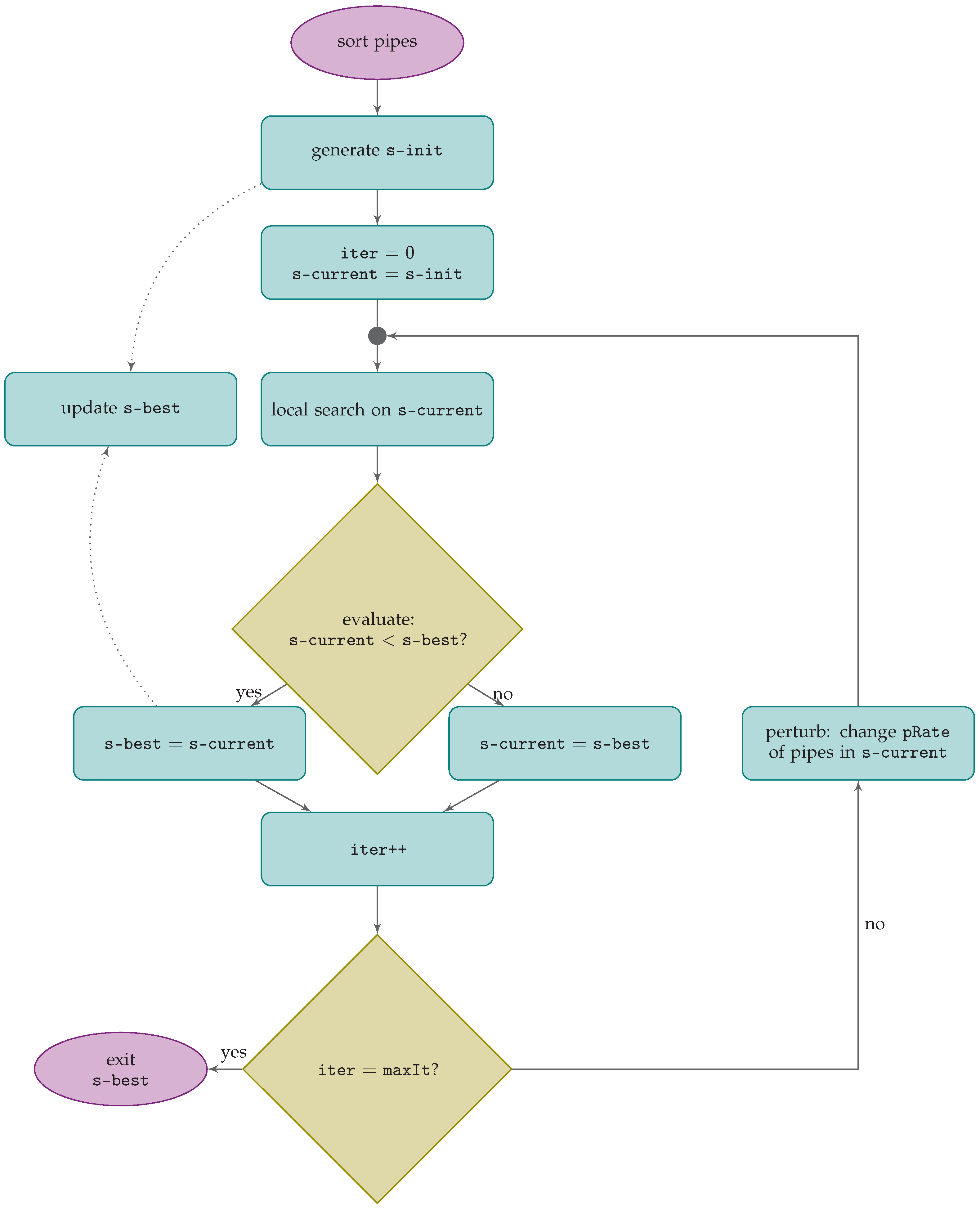
3.2. Detailed Algorithm Description
Sort
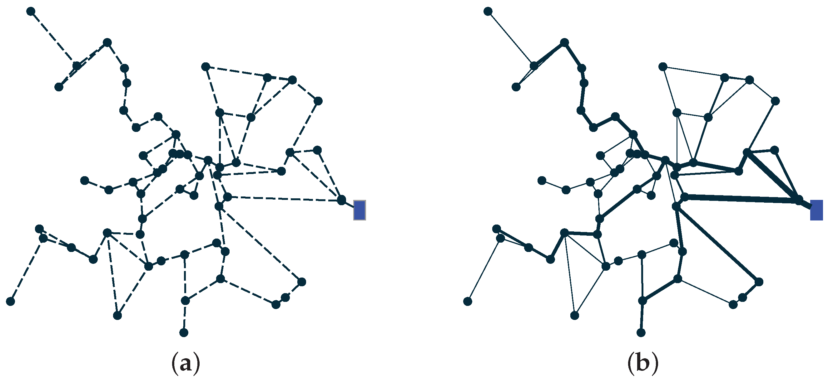
Initial Solution
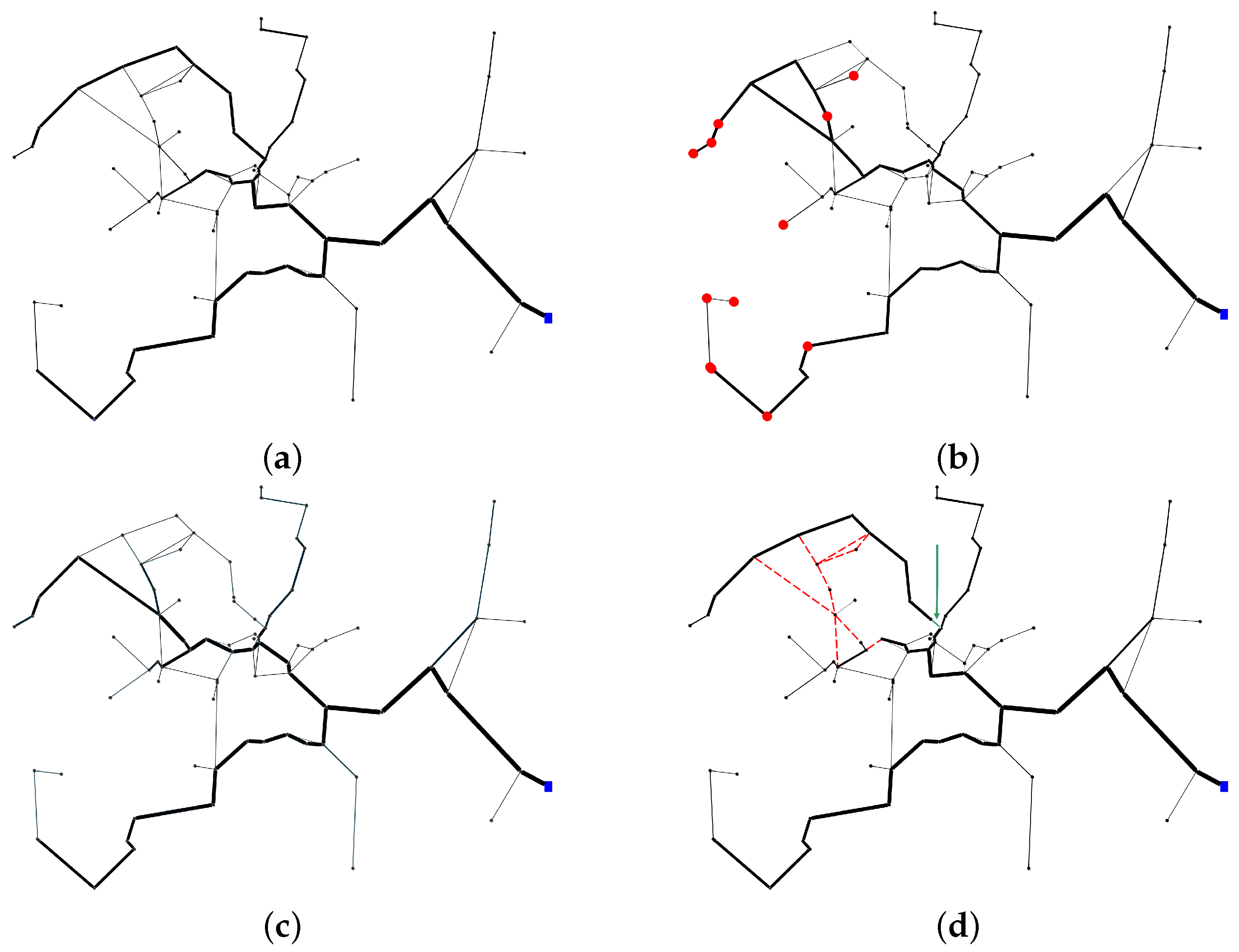
Local Search
Evaluation and Acceptance
Perturbation
Termination Criterion
3.3. Optimal Algorithm Configuration
3.3.1. Model on the Relative Cost
3.3.2. Model on the Running Time
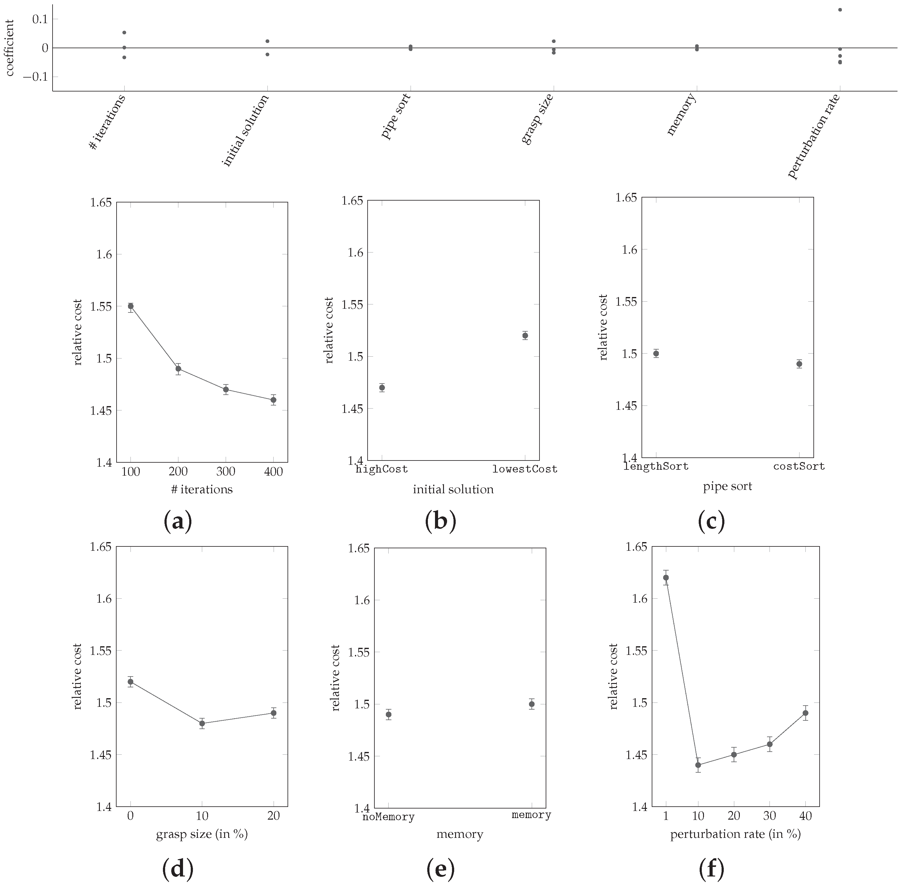
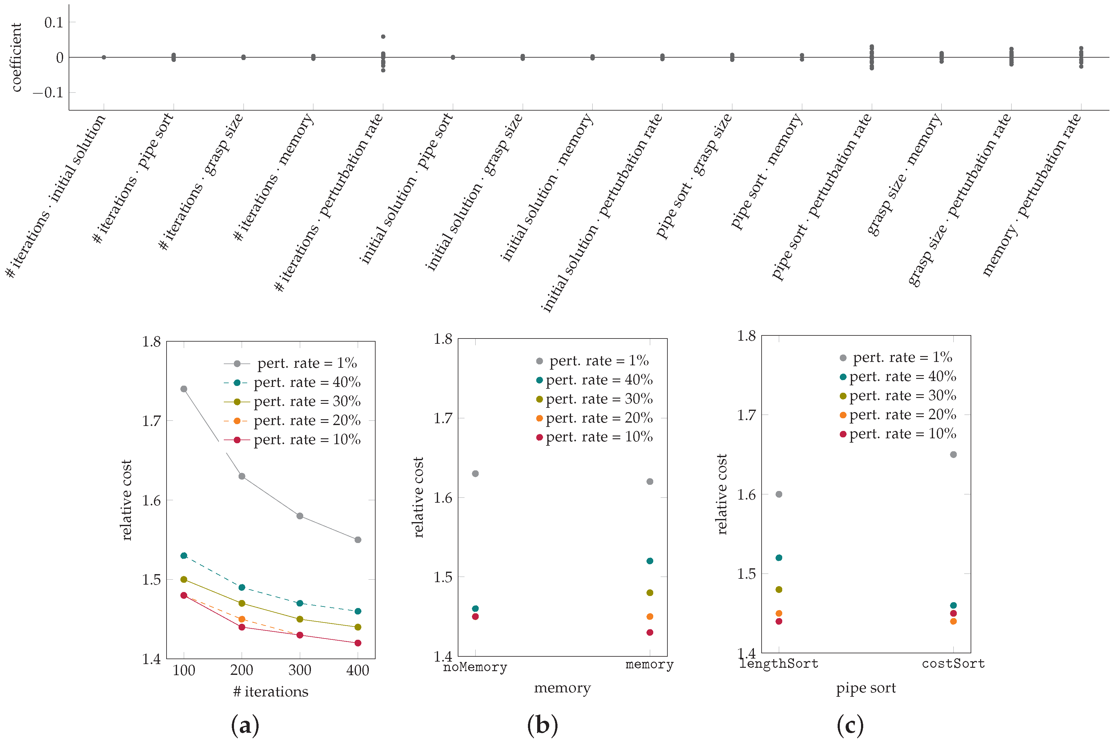
3.3.3. Influence of the Different Factors
Initial Solution
Pipe Sort
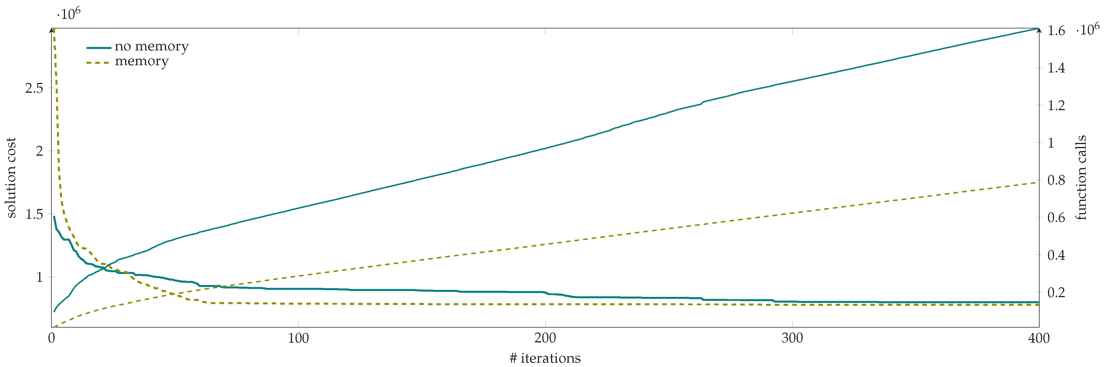
Local Search
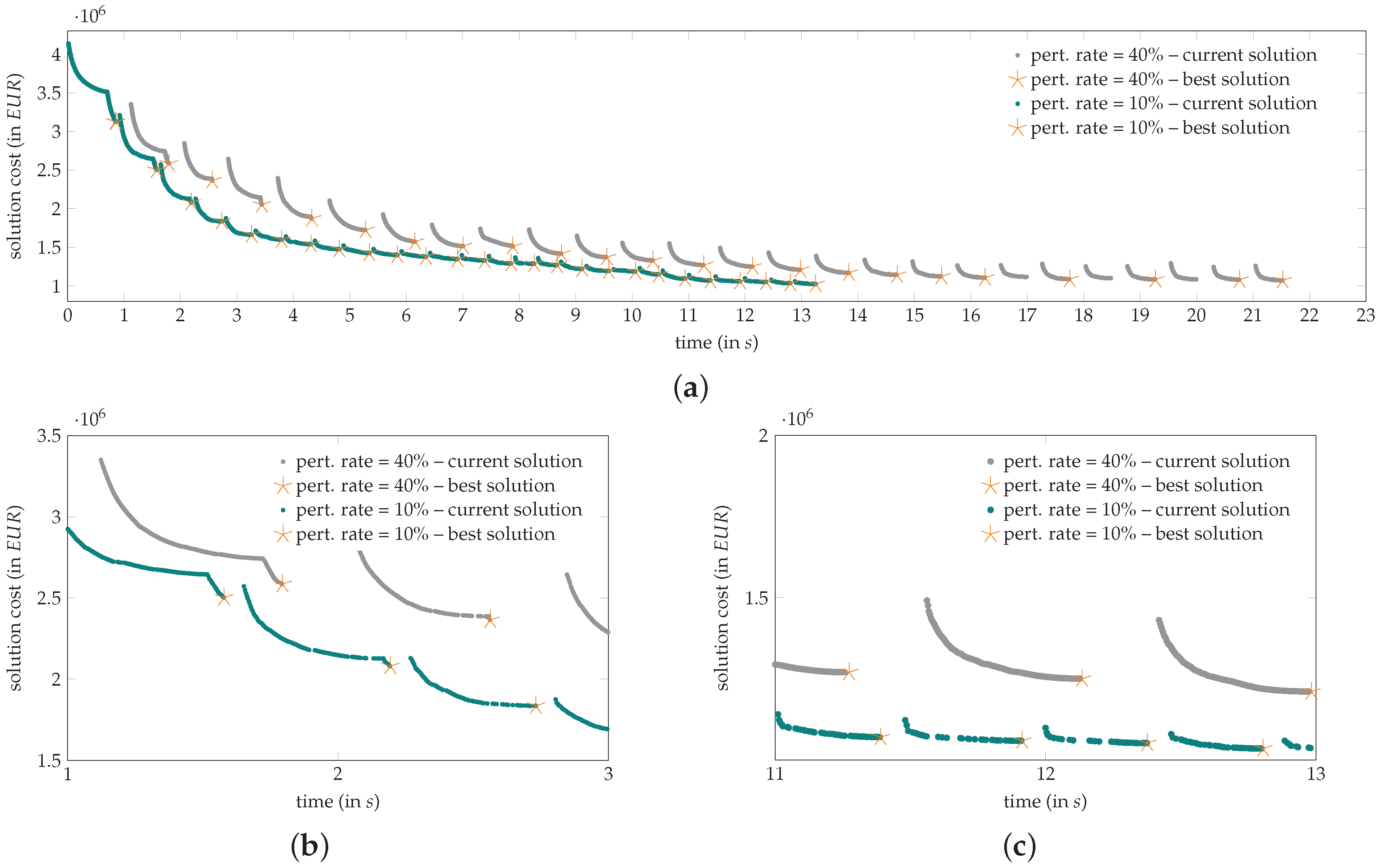
Perturbation
Termination Criterion
Network Size and Structure
4. Experimental Results
5. Conclusions
Acknowledgments
Author Contributions
Conflicts of Interest
Appendix A. Results of ILS on HydroGen Instances
| Network | # Function Evaluations | Mean # Iterations | Min Cost | Mean Cost | Max Cost | Stddev Cost |
| (in 106 ) | (in 106 ) | (in 106 ) | (in 106 ) | |||
| HG-MP-1-1 | 100,000 | 160 | 0.381 | 0.387 | 0.395 | 0.004 |
| HG-MP-1-1 | 300,000 | 574 | 0.380 | 0.385 | 0.391 | 0.003 |
| HG-MP-1-1 | 500,000 | 988 | 0.380 | 0.385 | 0.391 | 0.003 |
| HG-MP-1-1 | 1,000,000 | 2026 | 0.380 | 0.385 | 0.391 | 0.003 |
| HG-MP-1-1 | 1,500,000 | 3065 | 0.380 | 0.385 | 0.391 | 0.003 |
| HG-MP-1-2 | 100,000 | 155 | 0.348 | 0.361 | 0.414 | 0.019 |
| HG-MP-1-2 | 300,000 | 548 | 0.347 | 0.359 | 0.413 | 0.020 |
| HG-MP-1-2 | 500,000 | 938 | 0.347 | 0.359 | 0.413 | 0.020 |
| HG-MP-1-2 | 1,000,000 | 1904 | 0.347 | 0.359 | 0.413 | 0.020 |
| HG-MP-1-2 | 1,500,000 | 2871 | 0.346 | 0.359 | 0.413 | 0.020 |
| HG-MP-1-3 | 100,000 | 125 | 0.337 | 0.343 | 0.350 | 0.003 |
| HG-MP-1-3 | 300,000 | 482 | 0.335 | 0.339 | 0.342 | 0.002 |
| HG-MP-1-3 | 500,000 | 845 | 0.334 | 0.337 | 0.340 | 0.002 |
| HG-MP-1-3 | 1,000,000 | 1769 | 0.334 | 0.336 | 0.339 | 0.002 |
| HG-MP-1-3 | 1,500,000 | 2695 | 0.334 | 0.336 | 0.339 | 0.002 |
| HG-MP-1-4 | 100,000 | 161 | 0.340 | 0.355 | 0.382 | 0.011 |
| HG-MP-1-4 | 300,000 | 568 | 0.338 | 0.353 | 0.372 | 0.011 |
| HG-MP-1-4 | 500,000 | 974 | 0.338 | 0.352 | 0.366 | 0.009 |
| HG-MP-1-4 | 1,000,000 | 1997 | 0.338 | 0.352 | 0.365 | 0.009 |
| HG-MP-1-4 | 1,500,000 | 3017 | 0.338 | 0.351 | 0.365 | 0.009 |
| HG-MP-1-5 | 100,000 | 160 | 0.303 | 0.312 | 0.318 | 0.004 |
| HG-MP-1-5 | 300,000 | 547 | 0.298 | 0.310 | 0.318 | 0.006 |
| HG-MP-1-5 | 500,000 | 935 | 0.298 | 0.310 | 0.318 | 0.006 |
| HG-MP-1-5 | 1,000,000 | 1902 | 0.298 | 0.309 | 0.318 | 0.005 |
| HG-MP-1-5 | 1,500,000 | 2871 | 0.298 | 0.309 | 0.318 | 0.005 |
| HG-MP-2-1 | 100,000 | 149 | 0.319 | 0.395 | 0.441 | 0.036 |
| HG-MP-2-1 | 300,000 | 530 | 0.318 | 0.392 | 0.437 | 0.036 |
| HG-MP-2-1 | 500,000 | 917 | 0.318 | 0.388 | 0.431 | 0.034 |
| HG-MP-2-1 | 1,000,000 | 1881 | 0.318 | 0.387 | 0.431 | 0.034 |
| HG-MP-2-1 | 1,500,000 | 2849 | 0.318 | 0.387 | 0.431 | 0.034 |
| HG-MP-2-2 | 100,000 | 147 | 0.289 | 0.297 | 0.308 | 0.006 |
| HG-MP-2-2 | 300,000 | 521 | 0.289 | 0.294 | 0.305 | 0.005 |
| HG-MP-2-2 | 500,000 | 895 | 0.289 | 0.294 | 0.305 | 0.005 |
| HG-MP-2-2 | 1,000,000 | 1835 | 0.289 | 0.294 | 0.302 | 0.004 |
| HG-MP-2-2 | 1,500,000 | 2776 | 0.289 | 0.294 | 0.302 | 0.004 |
| HG-MP-2-3 | 100,000 | 150 | 0.248 | 0.286 | 0.313 | 0.022 |
| HG-MP-2-3 | 300,000 | 542 | 0.245 | 0.275 | 0.313 | 0.025 |
| HG-MP-2-3 | 500,000 | 943 | 0.245 | 0.274 | 0.313 | 0.025 |
| HG-MP-2-3 | 1,000,000 | 1953 | 0.245 | 0.274 | 0.313 | 0.025 |
| HG-MP-2-3 | 1,500,000 | 2959 | 0.245 | 0.269 | 0.313 | 0.023 |
| HG-MP-2-4 | 100,000 | 150 | 0.370 | 0.398 | 0.441 | 0.024 |
| HG-MP-2-4 | 300,000 | 544 | 0.369 | 0.390 | 0.437 | 0.023 |
| HG-MP-2-4 | 500,000 | 939 | 0.362 | 0.387 | 0.435 | 0.023 |
| HG-MP-2-4 | 1,000,000 | 1930 | 0.362 | 0.386 | 0.435 | 0.023 |
| HG-MP-2-4 | 1,500,000 | 2923 | 0.362 | 0.386 | 0.435 | 0.023 |
| HG-MP-2-5 | 100,000 | 139 | 0.349 | 0.387 | 0.444 | 0.043 |
| HG-MP-2-5 | 300,000 | 476 | 0.306 | 0.381 | 0.444 | 0.048 |
| HG-MP-2-5 | 500,000 | 814 | 0.306 | 0.381 | 0.444 | 0.048 |
| HG-MP-2-5 | 1,000,000 | 1655 | 0.306 | 0.379 | 0.440 | 0.048 |
| HG-MP-2-5 | 1,500,000 | 2497 | 0.305 | 0.374 | 0.438 | 0.052 |
| HG-MP-3-1 | 100,000 | 147 | 0.449 | 0.455 | 0.465 | 0.005 |
| HG-MP-3-1 | 300,000 | 513 | 0.446 | 0.451 | 0.459 | 0.004 |
| HG-MP-3-1 | 500,000 | 878 | 0.445 | 0.451 | 0.459 | 0.004 |
| HG-MP-3-1 | 1,000,000 | 1793 | 0.445 | 0.451 | 0.459 | 0.004 |
| HG-MP-3-1 | 1,500,000 | 2709 | 0.445 | 0.451 | 0.459 | 0.004 |
| HG-MP-3-2 | 100,000 | 141 | 0.321 | 0.367 | 0.431 | 0.049 |
| HG-MP-3-2 | 300,000 | 500 | 0.318 | 0.356 | 0.431 | 0.048 |
| HG-MP-3-2 | 500,000 | 866 | 0.318 | 0.355 | 0.431 | 0.048 |
| HG-MP-3-2 | 1,000,000 | 1785 | 0.318 | 0.355 | 0.431 | 0.048 |
| HG-MP-3-2 | 1,500,000 | 2707 | 0.318 | 0.354 | 0.431 | 0.048 |
| HG-MP-3-3 | 100,000 | 148 | 0.399 | 0.419 | 0.438 | 0.013 |
| HG-MP-3-3 | 300,000 | 536 | 0.398 | 0.417 | 0.437 | 0.013 |
| HG-MP-3-3 | 500,000 | 927 | 0.398 | 0.417 | 0.437 | 0.013 |
| HG-MP-3-3 | 1,000,000 | 1901 | 0.398 | 0.416 | 0.437 | 0.012 |
| HG-MP-3-3 | 1,500,000 | 2876 | 0.398 | 0.416 | 0.437 | 0.012 |
| HG-MP-3-4 | 100,000 | 135 | 0.343 | 0.351 | 0.357 | 0.004 |
| HG-MP-3-4 | 300,000 | 460 | 0.343 | 0.350 | 0.355 | 0.003 |
| HG-MP-3-4 | 500,000 | 786 | 0.343 | 0.349 | 0.355 | 0.004 |
| HG-MP-3-4 | 1,000,000 | 1605 | 0.343 | 0.349 | 0.353 | 0.003 |
| HG-MP-3-4 | 1,500,000 | 2427 | 0.343 | 0.349 | 0.353 | 0.003 |
| HG-MP-3-5 | 100,000 | 143 | 0.454 | 0.504 | 0.555 | 0.034 |
| HG-MP-3-5 | 300,000 | 521 | 0.442 | 0.484 | 0.555 | 0.041 |
| HG-MP-3-5 | 500,000 | 904 | 0.442 | 0.472 | 0.555 | 0.035 |
| HG-MP-3-5 | 1,000,000 | 1865 | 0.442 | 0.471 | 0.555 | 0.035 |
| HG-MP-3-5 | 1,500,000 | 2828 | 0.442 | 0.468 | 0.555 | 0.033 |
| HG-MP-4-1 | 100,000 | 47 | 0.810 | 0.855 | 0.903 | 0.029 |
| HG-MP-4-1 | 300,000 | 249 | 0.758 | 0.788 | 0.845 | 0.025 |
| HG-MP-4-1 | 500,000 | 461 | 0.755 | 0.781 | 0.842 | 0.027 |
| HG-MP-4-1 | 1,000,000 | 996 | 0.750 | 0.777 | 0.841 | 0.027 |
| HG-MP-4-1 | 1,500,000 | 1533 | 0.750 | 0.775 | 0.824 | 0.023 |
| HG-MP-4-2 | 100,000 | 46 | 0.813 | 0.866 | 0.956 | 0.037 |
| HG-MP-4-2 | 300,000 | 229 | 0.773 | 0.814 | 0.854 | 0.024 |
| HG-MP-4-2 | 500,000 | 420 | 0.770 | 0.810 | 0.849 | 0.024 |
| HG-MP-4-2 | 1,000,000 | 901 | 0.761 | 0.809 | 0.849 | 0.026 |
| HG-MP-4-2 | 1,500,000 | 1383 | 0.761 | 0.807 | 0.843 | 0.025 |
| HG-MP-4-3 | 100,000 | 45 | 0.709 | 0.736 | 0.776 | 0.023 |
| HG-MP-4-3 | 300,000 | 238 | 0.652 | 0.697 | 0.742 | 0.024 |
| HG-MP-4-3 | 500,000 | 443 | 0.642 | 0.690 | 0.732 | 0.026 |
| HG-MP-4-3 | 1,000,000 | 957 | 0.641 | 0.686 | 0.730 | 0.025 |
| HG-MP-4-3 | 1,500,000 | 1473 | 0.640 | 0.683 | 0.729 | 0.023 |
| HG-MP-4-4 | 100,000 | 47 | 0.781 | 0.824 | 0.887 | 0.033 |
| HG-MP-4-4 | 300,000 | 250 | 0.729 | 0.762 | 0.801 | 0.024 |
| HG-MP-4-4 | 500,000 | 463 | 0.725 | 0.759 | 0.796 | 0.024 |
| HG-MP-4-4 | 1,000,000 | 998 | 0.722 | 0.755 | 0.795 | 0.022 |
| HG-MP-4-4 | 1,500,000 | 1534 | 0.722 | 0.754 | 0.795 | 0.023 |
| HG-MP-4-5 | 100,000 | 47 | 0.649 | 0.677 | 0.707 | 0.018 |
| HG-MP-4-5 | 300,000 | 250 | 0.603 | 0.639 | 0.679 | 0.023 |
| HG-MP-4-5 | 500,000 | 456 | 0.599 | 0.631 | 0.678 | 0.025 |
| HG-MP-4-5 | 1,000,000 | 975 | 0.598 | 0.629 | 0.674 | 0.025 |
| HG-MP-4-5 | 1,500,000 | 1494 | 0.598 | 0.626 | 0.665 | 0.023 |
| HG-MP-5-1 | 100,000 | 44 | 0.867 | 0.944 | 1.002 | 0.039 |
| HG-MP-5-1 | 300,000 | 212 | 0.860 | 0.910 | 0.936 | 0.028 |
| HG-MP-5-1 | 500,000 | 384 | 0.859 | 0.903 | 0.935 | 0.027 |
| HG-MP-5-1 | 1,000,000 | 814 | 0.856 | 0.899 | 0.934 | 0.027 |
| HG-MP-5-1 | 1,500,000 | 1244 | 0.854 | 0.898 | 0.934 | 0.027 |
| HG-MP-5-2 | 100,000 | 45 | 0.669 | 0.738 | 0.828 | 0.050 |
| HG-MP-5-2 | 300,000 | 234 | 0.640 | 0.677 | 0.768 | 0.034 |
| HG-MP-5-2 | 500,000 | 432 | 0.631 | 0.671 | 0.768 | 0.037 |
| HG-MP-5-2 | 1,000,000 | 933 | 0.631 | 0.665 | 0.765 | 0.037 |
| HG-MP-5-2 | 1,500,000 | 1432 | 0.631 | 0.665 | 0.765 | 0.037 |
| HG-MP-5-3 | 100,000 | 43 | 0.876 | 0.935 | 0.994 | 0.032 |
| HG-MP-5-3 | 300,000 | 218 | 0.826 | 0.882 | 0.917 | 0.030 |
| HG-MP-5-3 | 500,000 | 399 | 0.825 | 0.872 | 0.905 | 0.030 |
| HG-MP-5-3 | 1,000,000 | 854 | 0.817 | 0.861 | 0.905 | 0.029 |
| HG-MP-5-3 | 1,500,000 | 1311 | 0.817 | 0.859 | 0.904 | 0.030 |
| HG-MP-5-4 | 100,000 | 47 | 0.693 | 0.731 | 0.785 | 0.028 |
| HG-MP-5-4 | 300,000 | 239 | 0.664 | 0.685 | 0.713 | 0.014 |
| HG-MP-5-4 | 500,000 | 439 | 0.664 | 0.680 | 0.712 | 0.014 |
| HG-MP-5-4 | 1,000,000 | 939 | 0.664 | 0.678 | 0.701 | 0.011 |
| HG-MP-5-4 | 1,500,000 | 1440 | 0.664 | 0.678 | 0.700 | 0.011 |
| HG-MP-5-5 | 100,000 | 46 | 0.705 | 0.765 | 0.842 | 0.044 |
| HG-MP-5-5 | 300,000 | 227 | 0.678 | 0.721 | 0.767 | 0.031 |
| HG-MP-5-5 | 500,000 | 418 | 0.675 | 0.720 | 0.767 | 0.031 |
| HG-MP-5-5 | 1,000,000 | 897 | 0.675 | 0.718 | 0.767 | 0.032 |
| HG-MP-5-5 | 1,500,000 | 1375 | 0.675 | 0.717 | 0.767 | 0.032 |
| HG-MP-6-1 | 100,000 | 44 | 0.633 | 0.668 | 0.712 | 0.025 |
| HG-MP-6-1 | 300,000 | 225 | 0.624 | 0.641 | 0.661 | 0.014 |
| HG-MP-6-1 | 500,000 | 413 | 0.619 | 0.636 | 0.659 | 0.013 |
| HG-MP-6-1 | 1,000,000 | 887 | 0.618 | 0.633 | 0.658 | 0.012 |
| HG-MP-6-1 | 1,500,000 | 1362 | 0.618 | 0.632 | 0.658 | 0.012 |
| HG-MP-6-2 | 100,000 | 47 | 0.836 | 0.870 | 0.896 | 0.023 |
| HG-MP-6-2 | 300,000 | 232 | 0.809 | 0.835 | 0.859 | 0.018 |
| HG-MP-6-2 | 500,000 | 420 | 0.791 | 0.828 | 0.857 | 0.020 |
| HG-MP-6-2 | 1,000,000 | 894 | 0.773 | 0.815 | 0.854 | 0.023 |
| HG-MP-6-2 | 1,500,000 | 1370 | 0.771 | 0.814 | 0.853 | 0.023 |
| HG-MP-6-3 | 100,000 | 47 | 0.963 | 0.987 | 1.043 | 0.022 |
| HG-MP-6-3 | 300,000 | 229 | 0.905 | 0.936 | 0.995 | 0.026 |
| HG-MP-6-3 | 500,000 | 420 | 0.898 | 0.923 | 0.960 | 0.019 |
| HG-MP-6-3 | 1,000,000 | 906 | 0.894 | 0.917 | 0.956 | 0.018 |
| HG-MP-6-3 | 1,500,000 | 1393 | 0.892 | 0.915 | 0.954 | 0.018 |
| HG-MP-6-4 | 100,000 | 46 | 0.754 | 0.782 | 0.855 | 0.027 |
| HG-MP-6-4 | 300,000 | 234 | 0.719 | 0.731 | 0.794 | 0.021 |
| HG-MP-6-4 | 500,000 | 433 | 0.711 | 0.722 | 0.773 | 0.017 |
| HG-MP-6-4 | 1,000,000 | 935 | 0.705 | 0.713 | 0.719 | 0.004 |
| HG-MP-6-4 | 1,500,000 | 1442 | 0.699 | 0.711 | 0.718 | 0.005 |
| HG-MP-6-5 | 100,000 | 47 | 0.797 | 0.830 | 0.904 | 0.033 |
| HG-MP-6-5 | 300,000 | 223 | 0.775 | 0.792 | 0.812 | 0.014 |
| HG-MP-6-5 | 500,000 | 402 | 0.772 | 0.789 | 0.812 | 0.014 |
| HG-MP-6-5 | 1,000,000 | 853 | 0.772 | 0.787 | 0.811 | 0.014 |
| HG-MP-6-5 | 1,500,000 | 1307 | 0.772 | 0.784 | 0.809 | 0.011 |
| HG-MP-7-1 | 100,000 | 21 | 1.189 | 1.377 | 1.557 | 0.126 |
| HG-MP-7-1 | 300,000 | 148 | 0.903 | 1.080 | 1.296 | 0.116 |
| HG-MP-7-1 | 500,000 | 291 | 0.901 | 1.060 | 1.291 | 0.120 |
| HG-MP-7-1 | 1,000,000 | 651 | 0.894 | 1.033 | 1.201 | 0.105 |
| HG-MP-7-1 | 1,500,000 | 1011 | 0.893 | 1.022 | 1.200 | 0.106 |
| HG-MP-7-2 | 100,000 | 22 | 1.032 | 1.077 | 1.115 | 0.028 |
| HG-MP-7-2 | 300,000 | 141 | 0.882 | 0.964 | 1.046 | 0.043 |
| HG-MP-7-2 | 500,000 | 271 | 0.874 | 0.952 | 1.027 | 0.042 |
| HG-MP-7-2 | 1,000,000 | 604 | 0.872 | 0.943 | 1.015 | 0.042 |
| HG-MP-7-2 | 1,500,000 | 940 | 0.858 | 0.938 | 1.010 | 0.045 |
| HG-MP-7-3 | 100,000 | 26 | 0.938 | 0.996 | 1.082 | 0.040 |
| HG-MP-7-3 | 300,000 | 141 | 0.774 | 0.825 | 0.890 | 0.037 |
| HG-MP-7-3 | 500,000 | 274 | 0.765 | 0.813 | 0.878 | 0.031 |
| HG-MP-7-3 | 1,000,000 | 611 | 0.762 | 0.807 | 0.875 | 0.032 |
| HG-MP-7-3 | 1,500,000 | 947 | 0.762 | 0.807 | 0.873 | 0.031 |
| HG-MP-7-4 | 100,000 | 23 | 1.074 | 1.167 | 1.276 | 0.060 |
| HG-MP-7-4 | 300,000 | 158 | 0.947 | 0.981 | 1.026 | 0.020 |
| HG-MP-7-4 | 500,000 | 305 | 0.943 | 0.975 | 1.023 | 0.020 |
| HG-MP-7-4 | 1,000,000 | 675 | 0.927 | 0.964 | 1.014 | 0.022 |
| HG-MP-7-4 | 1,500,000 | 1045 | 0.924 | 0.962 | 1.014 | 0.023 |
| HG-MP-7-5 | 100,000 | 24 | 0.774 | 0.863 | 0.976 | 0.053 |
| HG-MP-7-5 | 300,000 | 148 | 0.656 | 0.730 | 0.927 | 0.074 |
| HG-MP-7-5 | 500,000 | 287 | 0.654 | 0.714 | 0.904 | 0.072 |
| HG-MP-7-5 | 1,000,000 | 649 | 0.654 | 0.709 | 0.896 | 0.070 |
| HG-MP-7-5 | 1,500,000 | 1016 | 0.653 | 0.696 | 0.779 | 0.042 |
| HG-MP-8-1 | 100,000 | 22 | 0.995 | 1.075 | 1.191 | 0.057 |
| HG-MP-8-1 | 300,000 | 137 | 0.823 | 0.906 | 0.999 | 0.063 |
| HG-MP-8-1 | 500,000 | 264 | 0.812 | 0.892 | 0.988 | 0.059 |
| HG-MP-8-1 | 1,000,000 | 587 | 0.810 | 0.879 | 0.979 | 0.054 |
| HG-MP-8-1 | 1,500,000 | 914 | 0.807 | 0.875 | 0.975 | 0.053 |
| HG-MP-8-2 | 100,000 | 21 | 0.942 | 1.063 | 1.135 | 0.057 |
| HG-MP-8-2 | 300,000 | 126 | 0.883 | 0.953 | 1.024 | 0.045 |
| HG-MP-8-2 | 500,000 | 237 | 0.848 | 0.937 | 1.009 | 0.052 |
| HG-MP-8-2 | 1,000,000 | 521 | 0.834 | 0.919 | 0.969 | 0.047 |
| HG-MP-8-2 | 1,500,000 | 806 | 0.833 | 0.912 | 0.958 | 0.043 |
| HG-MP-8-3 | 100,000 | 23 | 0.903 | 1.013 | 1.127 | 0.068 |
| HG-MP-8-3 | 300,000 | 144 | 0.825 | 0.888 | 0.970 | 0.053 |
| HG-MP-8-3 | 500,000 | 275 | 0.820 | 0.882 | 0.953 | 0.051 |
| HG-MP-8-3 | 1,000,000 | 606 | 0.819 | 0.867 | 0.947 | 0.046 |
| HG-MP-8-3 | 1,500,000 | 943 | 0.818 | 0.866 | 0.946 | 0.046 |
| HG-MP-8-4 | 100,000 | 22 | 1.150 | 1.264 | 1.344 | 0.062 |
| HG-MP-8-4 | 300,000 | 141 | 0.891 | 1.019 | 1.180 | 0.081 |
| HG-MP-8-4 | 500,000 | 277 | 0.879 | 0.986 | 1.159 | 0.076 |
| HG-MP-8-4 | 1,000,000 | 621 | 0.868 | 0.974 | 1.128 | 0.073 |
| HG-MP-8-4 | 1,500,000 | 966 | 0.866 | 0.972 | 1.123 | 0.073 |
| HG-MP-8-5 | 100,000 | 24 | 1.226 | 1.360 | 1.441 | 0.061 |
| HG-MP-8-5 | 300,000 | 143 | 0.966 | 1.121 | 1.232 | 0.073 |
| HG-MP-8-5 | 500,000 | 276 | 0.948 | 1.091 | 1.185 | 0.064 |
| HG-MP-8-5 | 1,000,000 | 619 | 0.938 | 1.072 | 1.160 | 0.074 |
| HG-MP-8-5 | 1,500,000 | 962 | 0.934 | 1.055 | 1.140 | 0.070 |
| HG-MP-9-1 | 100,000 | 21 | 0.938 | 1.015 | 1.107 | 0.052 |
| HG-MP-9-1 | 300,000 | 140 | 0.867 | 0.896 | 0.921 | 0.019 |
| HG-MP-9-1 | 500,000 | 269 | 0.865 | 0.887 | 0.912 | 0.017 |
| HG-MP-9-1 | 1,000,000 | 597 | 0.854 | 0.879 | 0.894 | 0.015 |
| HG-MP-9-1 | 1,500,000 | 926 | 0.854 | 0.876 | 0.891 | 0.013 |
| HG-MP-9-2 | 100,000 | 26 | 1.083 | 1.141 | 1.221 | 0.035 |
| HG-MP-9-2 | 300,000 | 142 | 0.856 | 0.911 | 1.031 | 0.049 |
| HG-MP-9-2 | 500,000 | 272 | 0.841 | 0.889 | 1.009 | 0.047 |
| HG-MP-9-2 | 1,000,000 | 601 | 0.837 | 0.879 | 1.004 | 0.047 |
| HG-MP-9-2 | 1,500,000 | 930 | 0.837 | 0.877 | 1.000 | 0.046 |
| HG-MP-9-3 | 100,000 | 25 | 0.997 | 1.021 | 1.073 | 0.023 |
| HG-MP-9-3 | 300,000 | 143 | 0.878 | 0.915 | 0.971 | 0.026 |
| HG-MP-9-3 | 500,000 | 274 | 0.856 | 0.894 | 0.967 | 0.029 |
| HG-MP-9-3 | 1,000,000 | 607 | 0.846 | 0.887 | 0.960 | 0.031 |
| HG-MP-9-3 | 1,500,000 | 940 | 0.841 | 0.885 | 0.957 | 0.031 |
| HG-MP-9-4 | 100,000 | 24 | 0.812 | 0.867 | 0.933 | 0.042 |
| HG-MP-9-4 | 300,000 | 134 | 0.735 | 0.763 | 0.786 | 0.019 |
| HG-MP-9-4 | 500,000 | 254 | 0.730 | 0.752 | 0.778 | 0.017 |
| HG-MP-9-4 | 1,000,000 | 561 | 0.727 | 0.748 | 0.774 | 0.017 |
| HG-MP-9-4 | 1,500,000 | 871 | 0.725 | 0.746 | 0.771 | 0.017 |
| HG-MP-9-5 | 100,000 | 25 | 0.979 | 1.009 | 1.106 | 0.034 |
| HG-MP-9-5 | 300,000 | 136 | 0.909 | 0.941 | 0.984 | 0.018 |
| HG-MP-9-5 | 500,000 | 252 | 0.907 | 0.935 | 0.965 | 0.015 |
| HG-MP-9-5 | 1,000,000 | 548 | 0.905 | 0.919 | 0.934 | 0.008 |
| HG-MP-9-5 | 1,500,000 | 847 | 0.899 | 0.914 | 0.932 | 0.009 |
| HG-MP-10-1 | 100,000 | 16 | 1.181 | 1.260 | 1.337 | 0.052 |
| HG-MP-10-1 | 300,000 | 99 | 0.801 | 0.837 | 0.893 | 0.030 |
| HG-MP-10-1 | 500,000 | 208 | 0.779 | 0.809 | 0.856 | 0.023 |
| HG-MP-10-1 | 1,000,000 | 493 | 0.773 | 0.800 | 0.850 | 0.026 |
| HG-MP-10-1 | 1,500,000 | 780 | 0.772 | 0.798 | 0.847 | 0.025 |
| HG-MP-10-2 | 100,000 | 17 | 1.053 | 1.090 | 1.173 | 0.032 |
| HG-MP-10-2 | 300,000 | 100 | 0.851 | 0.893 | 0.937 | 0.026 |
| HG-MP-10-2 | 500,000 | 207 | 0.842 | 0.881 | 0.917 | 0.024 |
| HG-MP-10-2 | 1,000,000 | 487 | 0.830 | 0.873 | 0.905 | 0.025 |
| HG-MP-10-2 | 1,500,000 | 773 | 0.830 | 0.871 | 0.902 | 0.024 |
| HG-MP-10-3 | 100,000 | 18 | 1.083 | 1.138 | 1.223 | 0.042 |
| HG-MP-10-3 | 300,000 | 105 | 0.840 | 0.889 | 1.014 | 0.052 |
| HG-MP-10-3 | 500,000 | 223 | 0.801 | 0.862 | 0.978 | 0.050 |
| HG-MP-10-3 | 1,000,000 | 527 | 0.795 | 0.851 | 0.949 | 0.043 |
| HG-MP-10-3 | 1,500,000 | 838 | 0.793 | 0.848 | 0.939 | 0.041 |
| HG-MP-10-4 | 100,000 | 16 | 0.928 | 0.985 | 1.072 | 0.039 |
| HG-MP-10-4 | 300,000 | 90 | 0.741 | 0.802 | 0.861 | 0.043 |
| HG-MP-10-4 | 500,000 | 181 | 0.729 | 0.779 | 0.838 | 0.036 |
| HG-MP-10-4 | 1,000,000 | 428 | 0.725 | 0.770 | 0.837 | 0.034 |
| HG-MP-10-4 | 1,500,000 | 679 | 0.724 | 0.768 | 0.835 | 0.034 |
| HG-MP-10-5 | 100,000 | 18 | 1.124 | 1.236 | 1.372 | 0.067 |
| HG-MP-10-5 | 300,000 | 96 | 0.862 | 0.935 | 1.008 | 0.041 |
| HG-MP-10-5 | 500,000 | 206 | 0.859 | 0.899 | 0.957 | 0.031 |
| HG-MP-10-5 | 1,000,000 | 496 | 0.835 | 0.887 | 0.942 | 0.032 |
| HG-MP-10-5 | 1,500,000 | 792 | 0.834 | 0.883 | 0.926 | 0.029 |
| HG-MP-11-1 | 100,000 | 14 | 1.171 | 1.249 | 1.416 | 0.081 |
| HG-MP-11-1 | 300,000 | 100 | 0.941 | 0.990 | 1.084 | 0.043 |
| HG-MP-11-1 | 500,000 | 198 | 0.934 | 0.973 | 1.069 | 0.043 |
| HG-MP-11-1 | 1,000,000 | 452 | 0.916 | 0.960 | 1.049 | 0.040 |
| HG-MP-11-1 | 1,500,000 | 711 | 0.914 | 0.958 | 1.045 | 0.039 |
| HG-MP-11-2 | 100,000 | 13 | 1.147 | 1.241 | 1.431 | 0.075 |
| HG-MP-11-2 | 300,000 | 96 | 0.995 | 1.063 | 1.147 | 0.044 |
| HG-MP-11-2 | 500,000 | 190 | 0.976 | 1.035 | 1.125 | 0.045 |
| HG-MP-11-2 | 1,000,000 | 437 | 0.955 | 1.014 | 1.088 | 0.044 |
| HG-MP-11-2 | 1,500,000 | 688 | 0.944 | 1.005 | 1.083 | 0.045 |
| HG-MP-11-3 | 100,000 | 14 | 1.257 | 1.324 | 1.404 | 0.040 |
| HG-MP-11-3 | 300,000 | 89 | 0.913 | 0.991 | 1.043 | 0.040 |
| HG-MP-11-3 | 500,000 | 174 | 0.893 | 0.953 | 1.005 | 0.033 |
| HG-MP-11-3 | 1,000,000 | 395 | 0.874 | 0.939 | 0.999 | 0.033 |
| HG-MP-11-3 | 1,500,000 | 620 | 0.872 | 0.935 | 0.997 | 0.034 |
| HG-MP-11-4 | 100,000 | 16 | 1.038 | 1.149 | 1.273 | 0.081 |
| HG-MP-11-4 | 300,000 | 103 | 0.887 | 0.919 | 0.966 | 0.022 |
| HG-MP-11-4 | 500,000 | 205 | 0.875 | 0.903 | 0.941 | 0.018 |
| HG-MP-11-4 | 1,000,000 | 465 | 0.858 | 0.890 | 0.929 | 0.022 |
| HG-MP-11-4 | 1,500,000 | 725 | 0.856 | 0.885 | 0.922 | 0.018 |
| HG-MP-11-5 | 100,000 | 15 | 1.045 | 1.155 | 1.263 | 0.074 |
| HG-MP-11-5 | 300,000 | 103 | 0.958 | 1.018 | 1.124 | 0.043 |
| HG-MP-11-5 | 500,000 | 198 | 0.949 | 1.010 | 1.114 | 0.043 |
| HG-MP-11-5 | 1,000,000 | 440 | 0.949 | 1.005 | 1.104 | 0.041 |
| HG-MP-11-5 | 1,500,000 | 685 | 0.949 | 1.003 | 1.099 | 0.040 |
| HG-MP-12-1 | 100,000 | 15 | 1.414 | 1.467 | 1.559 | 0.046 |
| HG-MP-12-1 | 300,000 | 101 | 1.112 | 1.178 | 1.335 | 0.070 |
| HG-MP-12-1 | 500,000 | 199 | 1.109 | 1.152 | 1.261 | 0.050 |
| HG-MP-12-1 | 1,000,000 | 450 | 1.091 | 1.139 | 1.249 | 0.048 |
| HG-MP-12-1 | 1,500,000 | 702 | 1.078 | 1.135 | 1.243 | 0.049 |
| HG-MP-12-2 | 100,000 | 15 | 1.342 | 1.425 | 1.529 | 0.054 |
| HG-MP-12-2 | 300,000 | 92 | 1.142 | 1.191 | 1.257 | 0.029 |
| HG-MP-12-2 | 500,000 | 182 | 1.127 | 1.170 | 1.234 | 0.029 |
| HG-MP-12-2 | 1,000,000 | 414 | 1.112 | 1.146 | 1.204 | 0.029 |
| HG-MP-12-2 | 1,500,000 | 650 | 1.088 | 1.138 | 1.201 | 0.032 |
| HG-MP-12-3 | 100,000 | 17 | 1.195 | 1.247 | 1.299 | 0.035 |
| HG-MP-12-3 | 300,000 | 95 | 1.071 | 1.126 | 1.169 | 0.035 |
| HG-MP-12-3 | 500,000 | 186 | 1.057 | 1.100 | 1.146 | 0.032 |
| HG-MP-12-3 | 1,000,000 | 421 | 1.033 | 1.081 | 1.137 | 0.034 |
| HG-MP-12-3 | 1,500,000 | 661 | 1.026 | 1.071 | 1.133 | 0.035 |
| HG-MP-12-4 | 100,000 | 13 | 1.178 | 1.282 | 1.336 | 0.045 |
| HG-MP-12-4 | 300,000 | 89 | 1.037 | 1.085 | 1.136 | 0.036 |
| HG-MP-12-4 | 500,000 | 172 | 1.023 | 1.056 | 1.098 | 0.024 |
| HG-MP-12-4 | 1,000,000 | 388 | 1.006 | 1.035 | 1.076 | 0.024 |
| HG-MP-12-4 | 1,500,000 | 611 | 1.002 | 1.031 | 1.071 | 0.024 |
| HG-MP-12-5 | 100,000 | 14 | 1.114 | 1.249 | 1.380 | 0.067 |
| HG-MP-12-5 | 300,000 | 108 | 0.989 | 1.015 | 1.043 | 0.018 |
| HG-MP-12-5 | 500,000 | 213 | 0.972 | 1.006 | 1.039 | 0.020 |
| HG-MP-12-5 | 1,000,000 | 478 | 0.966 | 0.995 | 1.019 | 0.017 |
| HG-MP-12-5 | 1,500,000 | 745 | 0.920 | 0.988 | 1.018 | 0.027 |
| HG-MP-13-1 | 100,000 | 11 | 1.987 | 2.235 | 2.583 | 0.169 |
| HG-MP-13-1 | 300,000 | 61 | 1.371 | 1.457 | 1.537 | 0.059 |
| HG-MP-13-1 | 500,000 | 129 | 1.263 | 1.349 | 1.440 | 0.053 |
| HG-MP-13-1 | 1,000,000 | 323 | 1.223 | 1.285 | 1.400 | 0.053 |
| HG-MP-13-1 | 1,500,000 | 531 | 1.207 | 1.264 | 1.360 | 0.045 |
| HG-MP-13-2 | 100,000 | 11 | 1.918 | 2.066 | 2.247 | 0.096 |
| HG-MP-13-2 | 300,000 | 66 | 1.371 | 1.457 | 1.610 | 0.070 |
| HG-MP-13-2 | 500,000 | 139 | 1.304 | 1.372 | 1.490 | 0.048 |
| HG-MP-13-2 | 1,000,000 | 339 | 1.284 | 1.317 | 1.358 | 0.024 |
| HG-MP-13-2 | 1,500,000 | 547 | 1.268 | 1.301 | 1.349 | 0.026 |
| HG-MP-13-3 | 100,000 | 10 | 1.656 | 1.753 | 1.817 | 0.054 |
| HG-MP-13-3 | 300,000 | 64 | 1.173 | 1.244 | 1.343 | 0.048 |
| HG-MP-13-3 | 500,000 | 134 | 1.165 | 1.212 | 1.291 | 0.036 |
| HG-MP-13-3 | 1,000,000 | 324 | 1.131 | 1.184 | 1.242 | 0.028 |
| HG-MP-13-3 | 1,500,000 | 515 | 1.127 | 1.178 | 1.232 | 0.027 |
| HG-MP-13-4 | 100,000 | 11 | 2.010 | 2.158 | 2.411 | 0.133 |
| HG-MP-13-4 | 300,000 | 66 | 1.277 | 1.338 | 1.377 | 0.031 |
| HG-MP-13-4 | 500,000 | 142 | 1.256 | 1.285 | 1.318 | 0.021 |
| HG-MP-13-4 | 1,000,000 | 344 | 1.210 | 1.251 | 1.272 | 0.019 |
| HG-MP-13-4 | 1,500,000 | 551 | 1.205 | 1.235 | 1.269 | 0.019 |
| HG-MP-13-5 | 100,000 | 10 | 1.787 | 1.897 | 2.034 | 0.083 |
| HG-MP-13-5 | 300,000 | 67 | 1.266 | 1.363 | 1.498 | 0.082 |
| HG-MP-13-5 | 500,000 | 139 | 1.191 | 1.262 | 1.367 | 0.047 |
| HG-MP-13-5 | 1,000,000 | 338 | 1.153 | 1.195 | 1.275 | 0.037 |
| HG-MP-13-5 | 1,500,000 | 543 | 1.145 | 1.183 | 1.264 | 0.037 |
| HG-MP-14-1 | 100,000 | 9 | 1.559 | 1.623 | 1.727 | 0.059 |
| HG-MP-14-1 | 300,000 | 70 | 1.041 | 1.140 | 1.272 | 0.075 |
| HG-MP-14-1 | 500,000 | 150 | 1.026 | 1.102 | 1.257 | 0.072 |
| HG-MP-14-1 | 1,000,000 | 359 | 1.020 | 1.068 | 1.161 | 0.051 |
| HG-MP-14-1 | 1,500,000 | 573 | 1.013 | 1.048 | 1.117 | 0.038 |
| HG-MP-14-2 | 100,000 | 11 | 1.916 | 1.987 | 2.069 | 0.055 |
| HG-MP-14-2 | 300,000 | 65 | 1.442 | 1.585 | 1.754 | 0.107 |
| HG-MP-14-2 | 500,000 | 132 | 1.376 | 1.482 | 1.678 | 0.115 |
| HG-MP-14-2 | 1,000,000 | 306 | 1.283 | 1.359 | 1.455 | 0.051 |
| HG-MP-14-2 | 1,500,000 | 489 | 1.272 | 1.332 | 1.430 | 0.042 |
| HG-MP-14-3 | 100,000 | 10 | 1.590 | 1.649 | 1.744 | 0.045 |
| HG-MP-14-3 | 300,000 | 68 | 1.138 | 1.209 | 1.313 | 0.052 |
| HG-MP-14-3 | 500,000 | 143 | 1.127 | 1.173 | 1.277 | 0.040 |
| HG-MP-14-3 | 1,000,000 | 339 | 1.105 | 1.151 | 1.269 | 0.043 |
| HG-MP-14-3 | 1,500,000 | 538 | 1.101 | 1.143 | 1.242 | 0.037 |
| HG-MP-14-4 | 100,000 | 10 | 1.557 | 1.667 | 1.812 | 0.064 |
| HG-MP-14-4 | 300,000 | 71 | 1.131 | 1.208 | 1.256 | 0.038 |
| HG-MP-14-4 | 500,000 | 153 | 1.121 | 1.174 | 1.231 | 0.037 |
| HG-MP-14-4 | 1,000,000 | 364 | 1.096 | 1.155 | 1.224 | 0.045 |
| HG-MP-14-4 | 1,500,000 | 580 | 1.076 | 1.144 | 1.223 | 0.051 |
| HG-MP-14-5 | 100,000 | 11 | 1.267 | 1.398 | 1.679 | 0.118 |
| HG-MP-14-5 | 300,000 | 74 | 0.927 | 1.002 | 1.101 | 0.052 |
| HG-MP-14-5 | 500,000 | 156 | 0.898 | 0.961 | 1.043 | 0.039 |
| HG-MP-14-5 | 1,000,000 | 373 | 0.891 | 0.949 | 1.028 | 0.037 |
| HG-MP-14-5 | 1,500,000 | 591 | 0.889 | 0.943 | 1.022 | 0.035 |
| HG-MP-15-1 | 100,000 | 11 | 1.358 | 1.427 | 1.479 | 0.044 |
| HG-MP-15-1 | 300,000 | 74 | 1.159 | 1.212 | 1.287 | 0.037 |
| HG-MP-15-1 | 500,000 | 145 | 1.128 | 1.181 | 1.236 | 0.033 |
| HG-MP-15-1 | 1,000,000 | 334 | 1.085 | 1.153 | 1.188 | 0.030 |
| HG-MP-15-1 | 1,500,000 | 528 | 1.069 | 1.142 | 1.179 | 0.033 |
| HG-MP-15-2 | 100,000 | 10 | 1.814 | 2.138 | 2.325 | 0.152 |
| HG-MP-15-2 | 300,000 | 58 | 1.113 | 1.277 | 1.647 | 0.169 |
| HG-MP-15-2 | 500,000 | 121 | 1.064 | 1.131 | 1.362 | 0.083 |
| HG-MP-15-2 | 1,000,000 | 289 | 1.046 | 1.095 | 1.308 | 0.072 |
| HG-MP-15-2 | 1,500,000 | 463 | 1.039 | 1.086 | 1.283 | 0.068 |
| HG-MP-15-3 | 100,000 | 11 | 1.662 | 1.816 | 2.219 | 0.182 |
| HG-MP-15-3 | 300,000 | 71 | 1.280 | 1.346 | 1.414 | 0.044 |
| HG-MP-15-3 | 500,000 | 150 | 1.222 | 1.294 | 1.386 | 0.049 |
| HG-MP-15-3 | 1,000,000 | 357 | 1.210 | 1.272 | 1.348 | 0.044 |
| HG-MP-15-3 | 1,500,000 | 568 | 1.206 | 1.264 | 1.319 | 0.039 |
| HG-MP-15-4 | 100,000 | 11 | 1.368 | 1.447 | 1.620 | 0.072 |
| HG-MP-15-4 | 300,000 | 77 | 1.039 | 1.102 | 1.151 | 0.032 |
| HG-MP-15-4 | 500,000 | 158 | 1.020 | 1.069 | 1.130 | 0.028 |
| HG-MP-15-4 | 1,000,000 | 367 | 1.018 | 1.053 | 1.117 | 0.025 |
| HG-MP-15-4 | 1,500,000 | 577 | 1.018 | 1.049 | 1.117 | 0.026 |
| HG-MP-15-5 | 100,000 | 12 | 1.720 | 1.835 | 1.965 | 0.083 |
| HG-MP-15-5 | 300,000 | 78 | 1.448 | 1.479 | 1.546 | 0.030 |
| HG-MP-15-5 | 500,000 | 158 | 1.370 | 1.424 | 1.468 | 0.030 |
| HG-MP-15-5 | 1,000,000 | 363 | 1.315 | 1.394 | 1.446 | 0.036 |
| HG-MP-15-5 | 1,500,000 | 574 | 1.281 | 1.378 | 1.420 | 0.040 |
| HG-MP-16-1 | 100,000 | 9 | 2.600 | 2.700 | 2.881 | 0.077 |
| HG-MP-16-1 | 300,000 | 51 | 1.685 | 1.867 | 2.156 | 0.127 |
| HG-MP-16-1 | 500,000 | 111 | 1.487 | 1.677 | 1.984 | 0.170 |
| HG-MP-16-1 | 1,000,000 | 275 | 1.456 | 1.611 | 1.889 | 0.148 |
| HG-MP-16-1 | 1,500,000 | 441 | 1.451 | 1.585 | 1.864 | 0.141 |
| HG-MP-16-2 | 100,000 | 9 | 2.394 | 2.503 | 2.609 | 0.060 |
| HG-MP-16-2 | 300,000 | 50 | 1.729 | 1.806 | 1.893 | 0.052 |
| HG-MP-16-2 | 500,000 | 108 | 1.612 | 1.687 | 1.770 | 0.049 |
| HG-MP-16-2 | 1,000,000 | 267 | 1.557 | 1.633 | 1.697 | 0.045 |
| HG-MP-16-2 | 1,500,000 | 431 | 1.551 | 1.620 | 1.676 | 0.041 |
| HG-MP-16-3 | 100,000 | 8 | 2.362 | 2.446 | 2.560 | 0.066 |
| HG-MP-16-3 | 300,000 | 53 | 1.548 | 1.665 | 1.809 | 0.086 |
| HG-MP-16-3 | 500,000 | 119 | 1.464 | 1.558 | 1.638 | 0.051 |
| HG-MP-16-3 | 1,000,000 | 295 | 1.453 | 1.518 | 1.565 | 0.032 |
| HG-MP-16-3 | 1,500,000 | 477 | 1.440 | 1.498 | 1.538 | 0.030 |
| HG-MP-16-4 | 100,000 | 9 | 2.272 | 2.379 | 2.592 | 0.105 |
| HG-MP-16-4 | 300,000 | 52 | 1.367 | 1.546 | 1.726 | 0.114 |
| HG-MP-16-4 | 500,000 | 112 | 1.309 | 1.485 | 1.673 | 0.109 |
| HG-MP-16-4 | 1,000,000 | 273 | 1.278 | 1.420 | 1.596 | 0.101 |
| HG-MP-16-4 | 1,500,000 | 437 | 1.273 | 1.409 | 1.591 | 0.104 |
| HG-MP-16-5 | 100,000 | 9 | 2.968 | 3.128 | 3.268 | 0.096 |
| HG-MP-16-5 | 300,000 | 51 | 1.928 | 2.077 | 2.232 | 0.085 |
| HG-MP-16-5 | 500,000 | 112 | 1.815 | 1.893 | 1.977 | 0.051 |
| HG-MP-16-5 | 1,000,000 | 276 | 1.641 | 1.818 | 1.952 | 0.088 |
| HG-MP-16-5 | 1,500,000 | 444 | 1.626 | 1.804 | 1.929 | 0.086 |
| HG-MP-17-1 | 100,000 | 9 | 2.557 | 2.829 | 3.053 | 0.133 |
| HG-MP-17-1 | 300,000 | 54 | 1.749 | 1.899 | 2.048 | 0.094 |
| HG-MP-17-1 | 500,000 | 117 | 1.571 | 1.796 | 1.951 | 0.099 |
| HG-MP-17-1 | 1,000,000 | 288 | 1.402 | 1.720 | 1.893 | 0.139 |
| HG-MP-17-1 | 1,500,000 | 463 | 1.400 | 1.704 | 1.870 | 0.137 |
| HG-MP-17-2 | 100,000 | 8 | 2.727 | 2.873 | 3.186 | 0.141 |
| HG-MP-17-2 | 300,000 | 49 | 1.846 | 1.918 | 2.024 | 0.050 |
| HG-MP-17-2 | 500,000 | 106 | 1.686 | 1.784 | 1.851 | 0.049 |
| HG-MP-17-2 | 1,000,000 | 260 | 1.619 | 1.728 | 1.818 | 0.056 |
| HG-MP-17-2 | 1,500,000 | 418 | 1.611 | 1.715 | 1.798 | 0.054 |
| HG-MP-17-3 | 100,000 | 9 | 2.318 | 2.605 | 2.927 | 0.160 |
| HG-MP-17-3 | 300,000 | 46 | 1.592 | 1.761 | 1.894 | 0.090 |
| HG-MP-17-3 | 500,000 | 99 | 1.530 | 1.632 | 1.695 | 0.054 |
| HG-MP-17-3 | 1,000,000 | 243 | 1.481 | 1.566 | 1.652 | 0.052 |
| HG-MP-17-3 | 1,500,000 | 391 | 1.444 | 1.533 | 1.638 | 0.057 |
| HG-MP-17-4 | 100,000 | 8 | 2.761 | 2.939 | 3.147 | 0.104 |
| HG-MP-17-4 | 300,000 | 51 | 1.641 | 1.830 | 1.905 | 0.080 |
| HG-MP-17-4 | 500,000 | 115 | 1.614 | 1.771 | 1.851 | 0.071 |
| HG-MP-17-4 | 1,000,000 | 286 | 1.611 | 1.734 | 1.820 | 0.064 |
| HG-MP-17-4 | 1,500,000 | 461 | 1.606 | 1.725 | 1.814 | 0.065 |
| HG-MP-17-5 | 100,000 | 8 | 3.594 | 3.744 | 3.968 | 0.127 |
| HG-MP-17-5 | 300,000 | 49 | 1.951 | 2.142 | 2.411 | 0.126 |
| HG-MP-17-5 | 500,000 | 117 | 1.817 | 1.983 | 2.176 | 0.112 |
| HG-MP-17-5 | 1,000,000 | 299 | 1.759 | 1.908 | 2.062 | 0.099 |
| HG-MP-17-5 | 1,500,000 | 483 | 1.749 | 1.890 | 2.053 | 0.088 |
| HG-MP-18-1 | 100,000 | 9 | 2.378 | 2.513 | 2.744 | 0.131 |
| HG-MP-18-1 | 300,000 | 54 | 1.416 | 1.637 | 1.800 | 0.138 |
| HG-MP-18-1 | 500,000 | 115 | 1.311 | 1.529 | 1.703 | 0.127 |
| HG-MP-18-1 | 1,000,000 | 273 | 1.288 | 1.505 | 1.661 | 0.120 |
| HG-MP-18-1 | 1,500,000 | 433 | 1.284 | 1.498 | 1.655 | 0.119 |
| HG-MP-18-2 | 100,000 | 7 | 2.304 | 2.513 | 2.643 | 0.102 |
| HG-MP-18-2 | 300,000 | 46 | 1.322 | 1.444 | 1.566 | 0.069 |
| HG-MP-18-2 | 500,000 | 105 | 1.205 | 1.284 | 1.369 | 0.047 |
| HG-MP-18-2 | 1,000,000 | 264 | 1.173 | 1.238 | 1.312 | 0.044 |
| HG-MP-18-2 | 1,500,000 | 431 | 1.167 | 1.229 | 1.301 | 0.043 |
| HG-MP-18-3 | 100,000 | 8 | 2.955 | 3.084 | 3.182 | 0.069 |
| HG-MP-18-3 | 300,000 | 48 | 1.958 | 2.054 | 2.225 | 0.089 |
| HG-MP-18-3 | 500,000 | 108 | 1.848 | 1.934 | 2.098 | 0.064 |
| HG-MP-18-3 | 1,000,000 | 267 | 1.780 | 1.865 | 2.014 | 0.060 |
| HG-MP-18-3 | 1,500,000 | 429 | 1.760 | 1.845 | 2.000 | 0.060 |
| HG-MP-18-4 | 100,000 | 8 | 3.027 | 3.234 | 3.487 | 0.152 |
| HG-MP-18-4 | 300,000 | 48 | 1.827 | 1.969 | 2.261 | 0.111 |
| HG-MP-18-4 | 500,000 | 109 | 1.750 | 1.867 | 2.072 | 0.089 |
| HG-MP-18-4 | 1,000,000 | 278 | 1.686 | 1.813 | 1.976 | 0.076 |
| HG-MP-18-4 | 1,500,000 | 451 | 1.675 | 1.797 | 1.956 | 0.074 |
| HG-MP-18-5 | 100,000 | 8 | 2.714 | 2.920 | 3.291 | 0.197 |
| HG-MP-18-5 | 300,000 | 44 | 1.681 | 1.832 | 2.097 | 0.125 |
| HG-MP-18-5 | 500,000 | 99 | 1.624 | 1.705 | 1.813 | 0.060 |
| HG-MP-18-5 | 1,000,000 | 243 | 1.567 | 1.621 | 1.693 | 0.038 |
| HG-MP-18-5 | 1,500,000 | 392 | 1.563 | 1.605 | 1.683 | 0.038 |
| HG-MP-19-1 | 100,000 | 8 | 4.045 | 4.323 | 4.553 | 0.158 |
| HG-MP-19-1 | 300,000 | 40 | 2.553 | 2.694 | 2.801 | 0.076 |
| HG-MP-19-1 | 500,000 | 90 | 2.267 | 2.459 | 2.602 | 0.085 |
| HG-MP-19-1 | 1,000,000 | 233 | 2.194 | 2.369 | 2.531 | 0.095 |
| HG-MP-19-1 | 1,500,000 | 382 | 2.183 | 2.346 | 2.514 | 0.094 |
| HG-MP-19-2 | 100,000 | 7 | 4.696 | 5.144 | 5.656 | 0.269 |
| HG-MP-19-2 | 300,000 | 37 | 2.966 | 3.250 | 3.491 | 0.146 |
| HG-MP-19-2 | 500,000 | 82 | 2.689 | 2.857 | 3.411 | 0.220 |
| HG-MP-19-2 | 1,000,000 | 220 | 2.423 | 2.610 | 2.998 | 0.151 |
| HG-MP-19-2 | 1,500,000 | 366 | 2.386 | 2.537 | 2.905 | 0.141 |
| HG-MP-19-3 | 100,000 | 7 | 3.472 | 3.763 | 4.377 | 0.244 |
| HG-MP-19-3 | 300,000 | 41 | 2.327 | 2.400 | 2.496 | 0.049 |
| HG-MP-19-3 | 500,000 | 93 | 2.039 | 2.214 | 2.343 | 0.086 |
| HG-MP-19-3 | 1,000,000 | 235 | 1.973 | 2.124 | 2.242 | 0.104 |
| HG-MP-19-3 | 1,500,000 | 383 | 1.946 | 2.110 | 2.232 | 0.106 |
| HG-MP-19-4 | 100,000 | 7 | 3.132 | 3.578 | 4.251 | 0.341 |
| HG-MP-19-4 | 300,000 | 38 | 1.920 | 2.073 | 2.231 | 0.094 |
| HG-MP-19-4 | 500,000 | 89 | 1.837 | 1.942 | 2.077 | 0.078 |
| HG-MP-19-4 | 1,000,000 | 227 | 1.802 | 1.883 | 2.033 | 0.070 |
| HG-MP-19-4 | 1,500,000 | 367 | 1.761 | 1.846 | 1.938 | 0.054 |
| HG-MP-19-5 | 100,000 | 8 | 4.624 | 4.822 | 5.025 | 0.128 |
| HG-MP-19-5 | 300,000 | 37 | 2.740 | 3.008 | 3.238 | 0.173 |
| HG-MP-19-5 | 500,000 | 86 | 2.566 | 2.721 | 3.068 | 0.147 |
| HG-MP-19-5 | 1,000,000 | 225 | 2.413 | 2.580 | 2.984 | 0.157 |
| HG-MP-19-5 | 1,500,000 | 370 | 2.385 | 2.553 | 2.922 | 0.151 |
| HG-MP-20-1 | 100,000 | 7 | 6.054 | 6.502 | 7.171 | 0.406 |
| HG-MP-20-1 | 300,000 | 29 | 2.624 | 2.896 | 3.197 | 0.161 |
| HG-MP-20-1 | 500,000 | 64 | 1.951 | 2.338 | 2.534 | 0.189 |
| HG-MP-20-1 | 1,000,000 | 177 | 1.863 | 2.106 | 2.387 | 0.153 |
| HG-MP-20-1 | 1,500,000 | 298 | 1.815 | 2.079 | 2.353 | 0.158 |
| HG-MP-20-2 | 100,000 | 7 | 2.957 | 3.075 | 3.164 | 0.066 |
| HG-MP-20-2 | 300,000 | 44 | 2.011 | 2.115 | 2.213 | 0.059 |
| HG-MP-20-2 | 500,000 | 98 | 1.889 | 1.996 | 2.138 | 0.078 |
| HG-MP-20-2 | 1,000,000 | 249 | 1.755 | 1.922 | 2.065 | 0.086 |
| HG-MP-20-2 | 1,500,000 | 406 | 1.732 | 1.898 | 2.063 | 0.089 |
| HG-MP-20-3 | 100,000 | 7 | 3.866 | 4.021 | 4.160 | 0.092 |
| HG-MP-20-3 | 300,000 | 37 | 2.393 | 2.555 | 2.654 | 0.083 |
| HG-MP-20-3 | 500,000 | 82 | 2.281 | 2.442 | 2.583 | 0.096 |
| HG-MP-20-3 | 1,000,000 | 210 | 2.195 | 2.295 | 2.406 | 0.068 |
| HG-MP-20-3 | 1,500,000 | 347 | 2.191 | 2.264 | 2.375 | 0.057 |
| HG-MP-20-4 | 100,000 | 7 | 4.005 | 4.359 | 4.829 | 0.231 |
| HG-MP-20-4 | 300,000 | 39 | 2.576 | 2.848 | 3.328 | 0.264 |
| HG-MP-20-4 | 500,000 | 88 | 2.266 | 2.635 | 3.189 | 0.287 |
| HG-MP-20-4 | 1,000,000 | 229 | 2.114 | 2.279 | 2.572 | 0.118 |
| HG-MP-20-4 | 1,500,000 | 383 | 2.080 | 2.209 | 2.412 | 0.097 |
| HG-MP-20-5 | 100,000 | 8 | 4.392 | 4.575 | 4.767 | 0.107 |
| HG-MP-20-5 | 300,000 | 38 | 2.848 | 3.057 | 3.197 | 0.103 |
| HG-MP-20-5 | 500,000 | 85 | 2.355 | 2.641 | 2.962 | 0.170 |
| HG-MP-20-5 | 1,000,000 | 225 | 2.241 | 2.449 | 2.787 | 0.156 |
| HG-MP-20-5 | 1,500,000 | 371 | 2.218 | 2.416 | 2.758 | 0.161 |
| HG-MP-21-1 | 100,000 | 7 | 4.193 | 4.443 | 4.693 | 0.175 |
| HG-MP-21-1 | 300,000 | 36 | 2.283 | 2.694 | 2.926 | 0.198 |
| HG-MP-21-1 | 500,000 | 88 | 2.187 | 2.439 | 2.868 | 0.212 |
| HG-MP-21-1 | 1,000,000 | 232 | 2.069 | 2.278 | 2.648 | 0.189 |
| HG-MP-21-1 | 1,500,000 | 381 | 2.053 | 2.234 | 2.606 | 0.166 |
| HG-MP-21-2 | 100,000 | 7 | 4.089 | 4.551 | 4.738 | 0.184 |
| HG-MP-21-2 | 300,000 | 36 | 2.597 | 2.850 | 3.123 | 0.182 |
| HG-MP-21-2 | 500,000 | 85 | 2.423 | 2.526 | 2.809 | 0.117 |
| HG-MP-21-2 | 1,000,000 | 218 | 2.283 | 2.385 | 2.552 | 0.078 |
| HG-MP-21-2 | 1,500,000 | 357 | 2.258 | 2.363 | 2.506 | 0.073 |
| HG-MP-21-3 | 100,000 | 7 | 3.576 | 3.738 | 4.005 | 0.132 |
| HG-MP-21-3 | 300,000 | 38 | 2.359 | 2.511 | 2.732 | 0.110 |
| HG-MP-21-3 | 500,000 | 84 | 2.242 | 2.362 | 2.489 | 0.080 |
| HG-MP-21-3 | 1,000,000 | 211 | 2.150 | 2.287 | 2.419 | 0.078 |
| HG-MP-21-3 | 1,500,000 | 343 | 2.132 | 2.256 | 2.387 | 0.073 |
| HG-MP-21-4 | 100,000 | 7 | 4.035 | 4.421 | 4.864 | 0.229 |
| HG-MP-21-4 | 300,000 | 41 | 2.571 | 2.760 | 3.156 | 0.180 |
| HG-MP-21-4 | 500,000 | 91 | 2.430 | 2.584 | 3.027 | 0.172 |
| HG-MP-21-4 | 1,000,000 | 228 | 2.358 | 2.445 | 2.648 | 0.075 |
| HG-MP-21-4 | 1,500,000 | 371 | 2.326 | 2.418 | 2.569 | 0.061 |
| HG-MP-21-5 | 100,000 | 7 | 3.394 | 3.624 | 3.970 | 0.154 |
| HG-MP-21-5 | 300,000 | 36 | 1.934 | 2.090 | 2.285 | 0.110 |
| HG-MP-21-5 | 500,000 | 77 | 1.852 | 1.928 | 1.987 | 0.049 |
| HG-MP-21-5 | 1,000,000 | 187 | 1.811 | 1.871 | 1.932 | 0.041 |
| HG-MP-21-5 | 1,500,000 | 299 | 1.807 | 1.849 | 1.912 | 0.035 |
| HG-MP-22-1 | 100,000 | 6 | 4.360 | 4.724 | 4.947 | 0.192 |
| HG-MP-22-1 | 300,000 | 29 | 2.653 | 2.865 | 3.331 | 0.187 |
| HG-MP-22-1 | 500,000 | 67 | 2.433 | 2.570 | 2.876 | 0.123 |
| HG-MP-22-1 | 1,000,000 | 177 | 2.359 | 2.463 | 2.778 | 0.115 |
| HG-MP-22-1 | 1,500,000 | 292 | 2.320 | 2.406 | 2.700 | 0.105 |
| HG-MP-22-2 | 100,000 | 7 | 5.460 | 5.961 | 6.762 | 0.352 |
| HG-MP-22-2 | 300,000 | 33 | 2.952 | 3.298 | 3.512 | 0.180 |
| HG-MP-22-2 | 500,000 | 78 | 2.767 | 2.927 | 3.164 | 0.118 |
| HG-MP-22-2 | 1,000,000 | 200 | 2.585 | 2.759 | 2.881 | 0.081 |
| HG-MP-22-2 | 1,500,000 | 327 | 2.558 | 2.709 | 2.823 | 0.071 |
| HG-MP-22-3 | 100,000 | 6 | 5.746 | 6.032 | 6.365 | 0.189 |
| HG-MP-22-3 | 300,000 | 30 | 3.479 | 3.761 | 4.024 | 0.170 |
| HG-MP-22-3 | 500,000 | 69 | 3.111 | 3.348 | 3.703 | 0.186 |
| HG-MP-22-3 | 1,000,000 | 187 | 2.852 | 3.043 | 3.322 | 0.150 |
| HG-MP-22-3 | 1,500,000 | 313 | 2.795 | 2.990 | 3.214 | 0.128 |
| HG-MP-22-4 | 100,000 | 7 | 6.886 | 7.296 | 8.005 | 0.314 |
| HG-MP-22-4 | 300,000 | 29 | 3.900 | 4.310 | 4.769 | 0.275 |
| HG-MP-22-4 | 500,000 | 64 | 3.200 | 3.567 | 3.772 | 0.165 |
| HG-MP-22-4 | 1,000,000 | 175 | 2.965 | 3.211 | 3.428 | 0.136 |
| HG-MP-22-4 | 1,500,000 | 293 | 2.934 | 3.105 | 3.347 | 0.110 |
| HG-MP-22-5 | 100,000 | 7 | 5.056 | 5.460 | 5.878 | 0.262 |
| HG-MP-22-5 | 300,000 | 33 | 3.062 | 3.358 | 3.662 | 0.202 |
| HG-MP-22-5 | 500,000 | 74 | 2.788 | 3.003 | 3.200 | 0.130 |
| HG-MP-22-5 | 1,000,000 | 197 | 2.607 | 2.811 | 3.003 | 0.130 |
| HG-MP-22-5 | 1,500,000 | 327 | 2.595 | 2.777 | 2.940 | 0.116 |
| HG-MP-23-1 | 100,000 | 7 | 4.849 | 5.032 | 5.176 | 0.109 |
| HG-MP-23-1 | 300,000 | 32 | 3.097 | 3.298 | 3.583 | 0.161 |
| HG-MP-23-1 | 500,000 | 68 | 2.817 | 2.976 | 3.283 | 0.134 |
| HG-MP-23-1 | 1,000,000 | 175 | 2.698 | 2.852 | 3.083 | 0.125 |
| HG-MP-23-1 | 1,500,000 | 286 | 2.680 | 2.819 | 3.052 | 0.123 |
| HG-MP-23-2 | 100,000 | 6 | 5.228 | 5.433 | 5.812 | 0.172 |
| HG-MP-23-2 | 300,000 | 31 | 3.259 | 3.413 | 3.694 | 0.145 |
| HG-MP-23-2 | 500,000 | 68 | 2.822 | 3.093 | 3.386 | 0.153 |
| HG-MP-23-2 | 1,000,000 | 171 | 2.599 | 2.724 | 2.935 | 0.106 |
| HG-MP-23-2 | 1,500,000 | 281 | 2.546 | 2.678 | 2.918 | 0.102 |
| HG-MP-23-3 | 100,000 | 6 | 5.641 | 6.113 | 6.425 | 0.243 |
| HG-MP-23-3 | 300,000 | 29 | 3.180 | 3.592 | 3.844 | 0.205 |
| HG-MP-23-3 | 500,000 | 65 | 2.795 | 3.147 | 3.617 | 0.297 |
| HG-MP-23-3 | 1,000,000 | 170 | 2.517 | 2.688 | 2.912 | 0.134 |
| HG-MP-23-3 | 1,500,000 | 285 | 2.466 | 2.616 | 2.868 | 0.138 |
| HG-MP-23-4 | 100,000 | 6 | 6.290 | 6.716 | 7.035 | 0.251 |
| HG-MP-23-4 | 300,000 | 31 | 3.817 | 4.090 | 4.547 | 0.267 |
| HG-MP-23-4 | 500,000 | 70 | 2.920 | 3.375 | 3.832 | 0.259 |
| HG-MP-23-4 | 1,000,000 | 188 | 2.687 | 3.171 | 3.534 | 0.249 |
| HG-MP-23-4 | 1,500,000 | 310 | 2.676 | 3.120 | 3.482 | 0.245 |
| HG-MP-23-5 | 100,000 | 6 | 5.280 | 5.587 | 5.935 | 0.179 |
| HG-MP-23-5 | 300,000 | 31 | 3.160 | 3.399 | 3.676 | 0.126 |
| HG-MP-23-5 | 500,000 | 74 | 2.984 | 3.134 | 3.255 | 0.097 |
| HG-MP-23-5 | 1,000,000 | 192 | 2.785 | 2.981 | 3.233 | 0.116 |
| HG-MP-23-5 | 1,500,000 | 318 | 2.758 | 2.938 | 3.103 | 0.094 |
| HG-MP-24-1 | 100,000 | 6 | 5.318 | 5.584 | 5.862 | 0.154 |
| HG-MP-24-1 | 300,000 | 29 | 2.858 | 3.072 | 3.472 | 0.161 |
| HG-MP-24-1 | 500,000 | 66 | 2.485 | 2.783 | 2.990 | 0.130 |
| HG-MP-24-1 | 1,000,000 | 170 | 2.435 | 2.612 | 2.717 | 0.103 |
| HG-MP-24-1 | 1,500,000 | 279 | 2.424 | 2.556 | 2.677 | 0.087 |
| HG-MP-24-2 | 100,000 | 6 | 4.789 | 4.924 | 5.110 | 0.113 |
| HG-MP-24-2 | 300,000 | 30 | 2.877 | 3.070 | 3.257 | 0.100 |
| HG-MP-24-2 | 500,000 | 70 | 2.758 | 2.856 | 2.985 | 0.066 |
| HG-MP-24-2 | 1,000,000 | 177 | 2.661 | 2.741 | 2.834 | 0.053 |
| HG-MP-24-2 | 1,500,000 | 286 | 2.597 | 2.698 | 2.789 | 0.064 |
| HG-MP-24-3 | 100,000 | 6 | 4.805 | 4.967 | 5.251 | 0.121 |
| HG-MP-24-3 | 300,000 | 30 | 2.818 | 2.950 | 3.215 | 0.117 |
| HG-MP-24-3 | 500,000 | 71 | 2.560 | 2.672 | 2.947 | 0.108 |
| HG-MP-24-3 | 1,000,000 | 186 | 2.322 | 2.533 | 2.641 | 0.100 |
| HG-MP-24-3 | 1,500,000 | 306 | 2.300 | 2.507 | 2.628 | 0.098 |
| HG-MP-24-4 | 100,000 | 5 | 5.789 | 6.111 | 6.468 | 0.196 |
| HG-MP-24-4 | 300,000 | 27 | 2.739 | 3.016 | 3.278 | 0.160 |
| HG-MP-24-4 | 500,000 | 68 | 2.415 | 2.721 | 2.973 | 0.166 |
| HG-MP-24-4 | 1,000,000 | 182 | 2.373 | 2.545 | 2.673 | 0.093 |
| HG-MP-24-4 | 1,500,000 | 301 | 2.350 | 2.495 | 2.639 | 0.085 |
| HG-MP-24-5 | 100,000 | 6 | 5.640 | 6.032 | 6.278 | 0.222 |
| HG-MP-24-5 | 300,000 | 28 | 3.403 | 3.593 | 3.907 | 0.156 |
| HG-MP-24-5 | 500,000 | 70 | 3.026 | 3.249 | 3.510 | 0.157 |
| HG-MP-24-5 | 1,000,000 | 195 | 2.896 | 3.052 | 3.297 | 0.130 |
| HG-MP-24-5 | 1,500,000 | 325 | 2.839 | 3.002 | 3.239 | 0.120 |
| HG-MP-25-1 | 100,000 | 5 | 8.848 | 9.325 | 9.966 | 0.323 |
| HG-MP-25-1 | 300,000 | 23 | 4.380 | 4.719 | 5.144 | 0.251 |
| HG-MP-25-1 | 500,000 | 58 | 3.720 | 4.153 | 4.517 | 0.224 |
| HG-MP-25-1 | 1,000,000 | 162 | 3.601 | 3.825 | 3.948 | 0.114 |
| HG-MP-25-1 | 1,500,000 | 272 | 3.553 | 3.746 | 3.918 | 0.113 |
| HG-MP-25-2 | 100,000 | 5 | 7.750 | 8.258 | 8.815 | 0.347 |
| HG-MP-25-2 | 300,000 | 22 | 4.698 | 4.991 | 5.284 | 0.198 |
| HG-MP-25-2 | 500,000 | 53 | 4.079 | 4.441 | 4.669 | 0.186 |
| HG-MP-25-2 | 1,000,000 | 147 | 3.806 | 3.998 | 4.204 | 0.106 |
| HG-MP-25-2 | 1,500,000 | 250 | 3.721 | 3.919 | 4.092 | 0.099 |
| HG-MP-25-3 | 100,000 | 5 | 9.253 | 10.002 | 10.738 | 0.410 |
| HG-MP-25-3 | 300,000 | 23 | 4.541 | 5.301 | 5.869 | 0.330 |
| HG-MP-25-3 | 500,000 | 53 | 3.902 | 4.300 | 4.625 | 0.216 |
| HG-MP-25-3 | 1,000,000 | 144 | 3.548 | 3.814 | 4.157 | 0.196 |
| HG-MP-25-3 | 1,500,000 | 240 | 3.540 | 3.746 | 4.031 | 0.187 |
| HG-MP-25-4 | 100,000 | 6 | 10.317 | 10.770 | 11.175 | 0.250 |
| HG-MP-25-4 | 300,000 | 26 | 6.737 | 7.139 | 7.647 | 0.296 |
| HG-MP-25-4 | 500,000 | 57 | 5.489 | 6.035 | 6.360 | 0.258 |
| HG-MP-25-4 | 1,000,000 | 157 | 5.038 | 5.307 | 5.531 | 0.162 |
| HG-MP-25-4 | 1,500,000 | 267 | 4.911 | 5.171 | 5.340 | 0.153 |
| HG-MP-25-5 | 100,000 | 6 | 7.093 | 7.418 | 7.809 | 0.241 |
| HG-MP-25-5 | 300,000 | 26 | 4.073 | 4.571 | 4.953 | 0.271 |
| HG-MP-25-5 | 500,000 | 57 | 3.687 | 3.962 | 4.311 | 0.168 |
| HG-MP-25-5 | 1,000,000 | 154 | 3.490 | 3.623 | 3.705 | 0.063 |
| HG-MP-25-5 | 1,500,000 | 257 | 3.486 | 3.584 | 3.662 | 0.052 |
| HG-MP-26-1 | 100,000 | 5 | 8.500 | 8.946 | 9.759 | 0.346 |
| HG-MP-26-1 | 300,000 | 23 | 4.648 | 4.971 | 5.200 | 0.158 |
| HG-MP-26-1 | 500,000 | 55 | 4.033 | 4.301 | 4.724 | 0.185 |
| HG-MP-26-1 | 1,000,000 | 148 | 3.822 | 3.996 | 4.229 | 0.119 |
| HG-MP-26-1 | 1,500,000 | 244 | 3.801 | 3.947 | 4.128 | 0.096 |
| HG-MP-26-2 | 100,000 | 5 | 9.118 | 9.329 | 9.730 | 0.194 |
| HG-MP-26-2 | 300,000 | 25 | 4.657 | 5.186 | 5.594 | 0.287 |
| HG-MP-26-2 | 500,000 | 57 | 4.350 | 4.713 | 5.083 | 0.250 |
| HG-MP-26-2 | 1,000,000 | 150 | 4.088 | 4.255 | 4.495 | 0.133 |
| HG-MP-26-2 | 1,500,000 | 249 | 3.945 | 4.140 | 4.384 | 0.138 |
| HG-MP-26-3 | 100,000 | 5 | 8.255 | 8.520 | 8.806 | 0.193 |
| HG-MP-26-3 | 300,000 | 25 | 4.617 | 5.086 | 5.339 | 0.204 |
| HG-MP-26-3 | 500,000 | 58 | 4.115 | 4.450 | 4.747 | 0.207 |
| HG-MP-26-3 | 1,000,000 | 158 | 3.864 | 4.158 | 4.395 | 0.154 |
| HG-MP-26-3 | 1,500,000 | 263 | 3.785 | 4.074 | 4.278 | 0.153 |
| HG-MP-26-4 | 100,000 | 6 | 7.665 | 8.035 | 8.558 | 0.322 |
| HG-MP-26-4 | 300,000 | 26 | 4.660 | 5.010 | 5.257 | 0.170 |
| HG-MP-26-4 | 500,000 | 60 | 3.775 | 4.069 | 4.428 | 0.232 |
| HG-MP-26-4 | 1,000,000 | 163 | 3.370 | 3.644 | 4.081 | 0.224 |
| HG-MP-26-4 | 1,500,000 | 268 | 3.336 | 3.566 | 4.069 | 0.197 |
| HG-MP-26-5 | 100,000 | 5 | 10.069 | 10.737 | 12.767 | 0.775 |
| HG-MP-26-5 | 300,000 | 21 | 4.860 | 5.238 | 5.915 | 0.269 |
| HG-MP-26-5 | 500,000 | 50 | 4.257 | 4.488 | 4.959 | 0.201 |
| HG-MP-26-5 | 1,000,000 | 143 | 3.660 | 3.977 | 4.101 | 0.119 |
| HG-MP-26-5 | 1,500,000 | 243 | 3.623 | 3.916 | 3.996 | 0.105 |
| HG-MP-27-1 | 100,000 | 5 | 8.241 | 8.685 | 9.215 | 0.337 |
| HG-MP-27-1 | 300,000 | 24 | 3.929 | 4.726 | 5.600 | 0.457 |
| HG-MP-27-1 | 500,000 | 58 | 3.470 | 3.913 | 4.231 | 0.216 |
| HG-MP-27-1 | 1,000,000 | 153 | 3.240 | 3.647 | 4.113 | 0.253 |
| HG-MP-27-1 | 1,500,000 | 249 | 3.207 | 3.565 | 4.004 | 0.253 |
| HG-MP-27-2 | 100,000 | 5 | 8.303 | 8.962 | 9.490 | 0.339 |
| HG-MP-27-2 | 300,000 | 25 | 4.541 | 5.029 | 5.419 | 0.269 |
| HG-MP-27-2 | 500,000 | 59 | 3.987 | 4.495 | 4.944 | 0.308 |
| HG-MP-27-2 | 1,000,000 | 154 | 3.917 | 4.284 | 4.643 | 0.253 |
| HG-MP-27-2 | 1,500,000 | 251 | 3.872 | 4.189 | 4.570 | 0.239 |
| HG-MP-27-3 | 100,000 | 4 | 11.815 | 13.338 | 14.740 | 0.994 |
| HG-MP-27-3 | 300,000 | 18 | 3.595 | 4.198 | 4.941 | 0.446 |
| HG-MP-27-3 | 500,000 | 50 | 3.209 | 3.492 | 3.948 | 0.242 |
| HG-MP-27-3 | 1,000,000 | 143 | 3.127 | 3.307 | 3.690 | 0.179 |
| HG-MP-27-3 | 1,500,000 | 238 | 3.105 | 3.279 | 3.666 | 0.179 |
| HG-MP-27-4 | 100,000 | 5 | 10.554 | 11.139 | 12.130 | 0.483 |
| HG-MP-27-4 | 300,000 | 21 | 5.667 | 6.019 | 6.377 | 0.209 |
| HG-MP-27-4 | 500,000 | 50 | 4.849 | 5.259 | 5.543 | 0.213 |
| HG-MP-27-4 | 1,000,000 | 139 | 4.635 | 4.878 | 5.097 | 0.132 |
| HG-MP-27-4 | 1,500,000 | 231 | 4.586 | 4.779 | 4.931 | 0.118 |
| HG-MP-27-5 | 100,000 | 5 | 7.028 | 7.555 | 8.051 | 0.276 |
| HG-MP-27-5 | 300,000 | 25 | 4.292 | 4.711 | 4.983 | 0.187 |
| HG-MP-27-5 | 500,000 | 57 | 4.046 | 4.255 | 4.500 | 0.127 |
| HG-MP-27-5 | 1,000,000 | 151 | 3.750 | 4.021 | 4.166 | 0.117 |
| HG-MP-27-5 | 1,500,000 | 249 | 3.687 | 3.982 | 4.136 | 0.122 |
| HG-MP-28-1 | 100,000 | 5 | 14.302 | 15.472 | 16.244 | 0.586 |
| HG-MP-28-1 | 300,000 | 21 | 7.162 | 7.688 | 8.135 | 0.322 |
| HG-MP-28-1 | 500,000 | 47 | 6.129 | 6.440 | 7.299 | 0.336 |
| HG-MP-28-1 | 1,000,000 | 135 | 4.861 | 5.392 | 5.943 | 0.299 |
| HG-MP-28-1 | 1,500,000 | 234 | 4.825 | 5.281 | 5.700 | 0.265 |
| HG-MP-28-2 | 100,000 | 5 | 9.033 | 9.488 | 10.233 | 0.385 |
| HG-MP-28-2 | 300,000 | 22 | 5.498 | 5.831 | 6.135 | 0.208 |
| HG-MP-28-2 | 500,000 | 50 | 4.772 | 4.959 | 5.243 | 0.137 |
| HG-MP-28-2 | 1,000,000 | 135 | 4.170 | 4.428 | 4.722 | 0.167 |
| HG-MP-28-2 | 1,500,000 | 223 | 4.104 | 4.285 | 4.580 | 0.126 |
| HG-MP-28-3 | 100,000 | 5 | 11.762 | 12.479 | 13.480 | 0.559 |
| HG-MP-28-3 | 300,000 | 20 | 6.084 | 6.585 | 7.036 | 0.313 |
| HG-MP-28-3 | 500,000 | 48 | 5.228 | 5.461 | 5.791 | 0.145 |
| HG-MP-28-3 | 1,000,000 | 134 | 4.731 | 4.974 | 5.302 | 0.143 |
| HG-MP-28-3 | 1,500,000 | 224 | 4.655 | 4.893 | 5.152 | 0.121 |
| HG-MP-28-4 | 100,000 | 5 | 13.457 | 14.776 | 15.516 | 0.633 |
| HG-MP-28-4 | 300,000 | 21 | 7.402 | 7.974 | 8.524 | 0.355 |
| HG-MP-28-4 | 500,000 | 46 | 6.330 | 6.716 | 7.224 | 0.270 |
| HG-MP-28-4 | 1,000,000 | 127 | 5.502 | 5.815 | 6.458 | 0.242 |
| HG-MP-28-4 | 1,500,000 | 215 | 5.389 | 5.639 | 6.011 | 0.177 |
| HG-MP-28-5 | 100,000 | 5 | 11.717 | 12.876 | 13.534 | 0.547 |
| HG-MP-28-5 | 300,000 | 20 | 6.120 | 6.588 | 6.938 | 0.195 |
| HG-MP-28-5 | 500,000 | 47 | 5.200 | 5.612 | 5.856 | 0.186 |
| HG-MP-28-5 | 1,000,000 | 132 | 4.948 | 5.189 | 5.515 | 0.168 |
| HG-MP-28-5 | 1,500,000 | 225 | 4.838 | 5.078 | 5.427 | 0.175 |
| HG-MP-29-1 | 100,000 | 4 | 14.410 | 14.959 | 15.641 | 0.391 |
| HG-MP-29-1 | 300,000 | 17 | 6.257 | 6.851 | 7.230 | 0.274 |
| HG-MP-29-1 | 500,000 | 41 | 5.417 | 5.735 | 6.186 | 0.244 |
| HG-MP-29-1 | 1,000,000 | 117 | 4.778 | 5.062 | 5.592 | 0.247 |
| HG-MP-29-1 | 1,500,000 | 198 | 4.573 | 4.884 | 5.499 | 0.240 |
| HG-MP-29-2 | 100,000 | 5 | 16.444 | 17.201 | 17.823 | 0.481 |
| HG-MP-29-2 | 300,000 | 20 | 8.337 | 9.329 | 11.109 | 0.855 |
| HG-MP-29-2 | 500,000 | 44 | 6.069 | 7.131 | 8.155 | 0.664 |
| HG-MP-29-2 | 1,000,000 | 122 | 5.017 | 5.703 | 6.354 | 0.431 |
| HG-MP-29-2 | 1,500,000 | 207 | 4.849 | 5.560 | 6.256 | 0.433 |
| HG-MP-29-3 | 100,000 | 5 | 14.855 | 15.869 | 16.619 | 0.623 |
| HG-MP-29-3 | 300,000 | 19 | 7.681 | 8.655 | 9.365 | 0.575 |
| HG-MP-29-3 | 500,000 | 43 | 5.592 | 6.125 | 6.899 | 0.345 |
| HG-MP-29-3 | 1,000,000 | 128 | 5.057 | 5.268 | 5.750 | 0.208 |
| HG-MP-29-3 | 1,500,000 | 220 | 4.952 | 5.142 | 5.552 | 0.180 |
| HG-MP-29-4 | 100,000 | 5 | 10.829 | 11.970 | 12.557 | 0.583 |
| HG-MP-29-4 | 300,000 | 20 | 5.808 | 6.507 | 7.228 | 0.437 |
| HG-MP-29-4 | 500,000 | 47 | 4.842 | 5.515 | 6.538 | 0.500 |
| HG-MP-29-4 | 1,000,000 | 130 | 4.634 | 4.965 | 5.531 | 0.306 |
| HG-MP-29-4 | 1,500,000 | 215 | 4.617 | 4.789 | 5.139 | 0.164 |
| HG-MP-29-5 | 100,000 | 5 | 12.781 | 13.652 | 14.963 | 0.558 |
| HG-MP-29-5 | 300,000 | 21 | 6.976 | 7.236 | 7.459 | 0.174 |
| HG-MP-29-5 | 500,000 | 50 | 5.965 | 6.242 | 6.573 | 0.219 |
| HG-MP-29-5 | 1,000,000 | 137 | 5.492 | 5.740 | 6.058 | 0.170 |
| HG-MP-29-5 | 1,500,000 | 230 | 5.438 | 5.619 | 5.932 | 0.150 |
| HG-MP-30-1 | 100,000 | 5 | 12.217 | 13.480 | 14.729 | 0.911 |
| HG-MP-30-1 | 300,000 | 19 | 6.766 | 7.087 | 7.380 | 0.184 |
| HG-MP-30-1 | 500,000 | 44 | 5.801 | 6.267 | 6.518 | 0.221 |
| HG-MP-30-1 | 1,000,000 | 120 | 5.097 | 5.470 | 5.839 | 0.222 |
| HG-MP-30-1 | 1,500,000 | 204 | 4.878 | 5.298 | 5.759 | 0.235 |
| HG-MP-30-2 | 100,000 | 4 | 13.930 | 15.653 | 16.982 | 0.971 |
| HG-MP-30-2 | 300,000 | 17 | 6.030 | 6.555 | 7.026 | 0.278 |
| HG-MP-30-2 | 500,000 | 43 | 4.803 | 5.357 | 5.764 | 0.287 |
| HG-MP-30-2 | 1,000,000 | 118 | 4.242 | 4.749 | 5.238 | 0.293 |
| HG-MP-30-2 | 1,500,000 | 195 | 4.142 | 4.585 | 5.019 | 0.271 |
| HG-MP-30-3 | 100,000 | 5 | 11.964 | 12.701 | 13.300 | 0.358 |
| HG-MP-30-3 | 300,000 | 20 | 7.102 | 7.397 | 7.777 | 0.240 |
| HG-MP-30-3 | 500,000 | 46 | 5.744 | 6.096 | 6.395 | 0.226 |
| HG-MP-30-3 | 1,000,000 | 127 | 4.891 | 5.412 | 6.154 | 0.318 |
| HG-MP-30-3 | 1,500,000 | 214 | 4.820 | 5.301 | 5.885 | 0.278 |
| HG-MP-30-4 | 100,000 | 5 | 9.219 | 9.739 | 10.796 | 0.445 |
| HG-MP-30-4 | 300,000 | 20 | 5.297 | 5.783 | 6.497 | 0.317 |
| HG-MP-30-4 | 500,000 | 49 | 4.966 | 5.413 | 5.974 | 0.327 |
| HG-MP-30-4 | 1,000,000 | 128 | 4.530 | 4.847 | 5.207 | 0.260 |
| HG-MP-30-4 | 1,500,000 | 215 | 4.432 | 4.629 | 5.021 | 0.169 |
| HG-MP-30-5 | 100,000 | 4 | 12.417 | 13.202 | 13.632 | 0.362 |
| HG-MP-30-5 | 300,000 | 17 | 5.356 | 5.751 | 6.004 | 0.220 |
| HG-MP-30-5 | 500,000 | 43 | 4.525 | 4.804 | 5.023 | 0.175 |
| HG-MP-30-5 | 1,000,000 | 123 | 4.096 | 4.425 | 4.759 | 0.214 |
| HG-MP-30-5 | 1,500,000 | 205 | 4.051 | 4.323 | 4.681 | 0.205 |
References
- World Health Organization. Guidelines for Drinking-Water Quality, 4th ed.; World Health Organization (WHO): Geneva, Switzerland, 2011. [Google Scholar]
- Mays, L.; Koutsoyiannis, D.; Angelakis, A. A brief history of urban water supply in antiquity. Water Supply 2007, 7, 1–12. [Google Scholar] [CrossRef]
- United Nations Children’s Emergency Fund; World Health Organization (WHO). Progress on Drinking Water and Sanitation; WHO: Geneva, Switzerland, 2012. [Google Scholar]
- Grayman, W.; Loucks, D.; Saito, L. Towards a Sustainable Water Future: Visions for 2050; American Society of Civil Engineers (ASCE): Reston, VA, USA, 2012. [Google Scholar]
- Alperovits, A.; Shamir, U. Design of optimal water distribution systems. Water Resour. Res. 1977, 13, 885–900. [Google Scholar] [CrossRef]
- Quindry, G.; Liebman, J.; Brill, E. Optimization of looped water distribution systems. J. Environ. Eng. Div. 1981, 107, 665–679. [Google Scholar]
- Kessler, A.; Shamir, U. Analysis of the linear programming gradient method for optimal design of water supply networks. Water Resour. Res. 1989, 25, 1469–1480. [Google Scholar] [CrossRef]
- Shamir, U. Optimal design and operation of water distribution systems. Water Resour. Res. 1974, 10, 27–36. [Google Scholar] [CrossRef]
- El-Bahrawy, A.; Smith, A. A methodology for optimal design of pipe distribution networks. Can. J. Civ. Eng. 1987, 14, 207–215. [Google Scholar] [CrossRef]
- Fujiwara, O.; Khang, D. A two-phase decompostion method for optimal design of looped water distribution networks. Water Resour. Res. 1990, 26, 539–549. [Google Scholar] [CrossRef]
- Duan, N.; Mays, L.; Lansey, K. Optimal reliability-based design of pumping and distribution systems. J. Hydraul. Eng. 1990, 116, 249–268. [Google Scholar] [CrossRef]
- Rossman, L. EPANET 2: Users Manual; Environmental Protection Agency: Washington, DC, USA, 2000. [Google Scholar]
- Loganathan, G.; Greene, J.; Ahn, T. Design heuristic for globally minimum cost water distribution systems. J. Water Resour. Plan. Manag. 1995, 121, 182–192. [Google Scholar] [CrossRef]
- Cunha, M.; Sousa, J. Hydraulic infrastructures design using simulated annealing. J. Infrastruct. Syst. 2001, 7, 32–39. [Google Scholar] [CrossRef]
- Cunha, M.; Ribeiro, L. Tabu search algorithms for water network optimization. Eur. J. Oper. Res. 2004, 157, 746–758. [Google Scholar] [CrossRef]
- Maier, H.; Simpson, A.; Zecchin, A.; Foong, W.; Phang, K.; Seah, H.; Tan, C. Ant colony optimization for design of water distribution systems. J. Water Resour. Plan. Manag. 2003, 129, 200–209. [Google Scholar] [CrossRef]
- Zecchin, A.; Simpson, A.; Maier, H.; Nixon, J. Parametric study for an ant algorithm applied to water distribution system optimization. IEEE Trans. Evol. Comput. 2005, 9, 175–191. [Google Scholar] [CrossRef]
- Dandy, G.; Simpson, A.; Murphy, L. An improved genetic algorithm for pipe network optimisation. Water Resour. Res. 1996, 32, 449–458. [Google Scholar] [CrossRef]
- Gupta, I.; Gupta, A.; Khanna, P. Genetic algorithm for optimization of water distribution systems. Environ. Model. Softw. 1999, 14, 437–446. [Google Scholar] [CrossRef]
- Bi, W.; Dandy, G.; Maier, R. Improved genetic algorithm optimization of water distribution system design by incorporating domain knowledge. Environ. Model. Softw. 2015, 69, 370–381. [Google Scholar] [CrossRef]
- Lin, M.; Liu, Y.; Liu, G.; Chu, C. Scatter search heuristic for least-cost design of water distribution networks. Eng. Optim. 2007, 39, 857–876. [Google Scholar] [CrossRef]
- Vasan, A.; Simonovic, S. Optimization of water distribution network design using differential evolution. J. Water Resour. Plan. Manag. 2010, 136, 279–287. [Google Scholar] [CrossRef]
- Marchi, A.; Dandy, G.; Wilkins, A.; Rohrlach, H. Methodology for comparing evolutionary algorithms for optimization of water distribution systems. J. Water Resour. Plan. Manag. 2014, 140, 22–31. [Google Scholar] [CrossRef]
- De Corte, A.; Sörensen, K. Optimisation of gravity-fed water distribution network design: A critical review. Eur. J. Oper. Res. 2013, 228, 1–10. [Google Scholar] [CrossRef]
- Farmani, R.; Walters, G.; Savic, D. Trade-off between total cost and reliability for Anytown water distribution network. J. Water Resour. Plan. Manag. 2005, 131, 161–171. [Google Scholar] [CrossRef]
- Bragalli, C.; D’Ambrosio, C.; Lee, J.; Lodi, A.; Toth, P. On the optimal design of water distribution networks: A practical MINLP approach. Optim. Eng. 2012, 13, 219–246. [Google Scholar] [CrossRef]
- De Corte, A.; Sörensen, K. HydroGen: An artificial water distribution network generator. Water Resour. Manag. 2014, 28, 333–350. [Google Scholar] [CrossRef]
- Yates, D.; Templeman, A.; Boffey, T. The computational complexity of the problem of determining least capital cost designs for water supply networks. Eng. Optim. 1984, 7, 143–155. [Google Scholar] [CrossRef]
- Lourenço, H.; Martin, O.; Stützle, T. Chapter 11: Iterated local search. In Handbook of Metaheuristics; Springer: New York, NY, USA, 2003; pp. 320–353. [Google Scholar]
- López-Ibáñez, M. Operational Optimisation of Water Distribution Networks. Ph.D. Thesis, School of Engineering and the Built Environment, Edinburgh Napier University (UK), Edinburgh, UK, 2009. [Google Scholar]
- López-Ibáñez, M. Extended EPANET Toolkit. Available online: http://iridia.ulb.ac.be/ manuel/epanetlinux. html (accessed on 18 August 2016).
- Maier, H.; Kapelan, Z.; Kasprzyk, J.; Kollat, J.; Matott, L.; Cunha, M.; Dandy, G.; Gibbs, M.; Keedwell, E.; Marchi, A.; et al. Evolutionary algorithms and other metaheuristics in water resources: Current status, research challenges and future directions. Environ. Model. Softw. 2014, 62, 271–299. [Google Scholar] [CrossRef] [Green Version]
- De Corte, A.; Sörensen, K. Hydrogen. Available online: http://antor.uantwerpen.be/hydrogen (accessed on 18 August 2016).


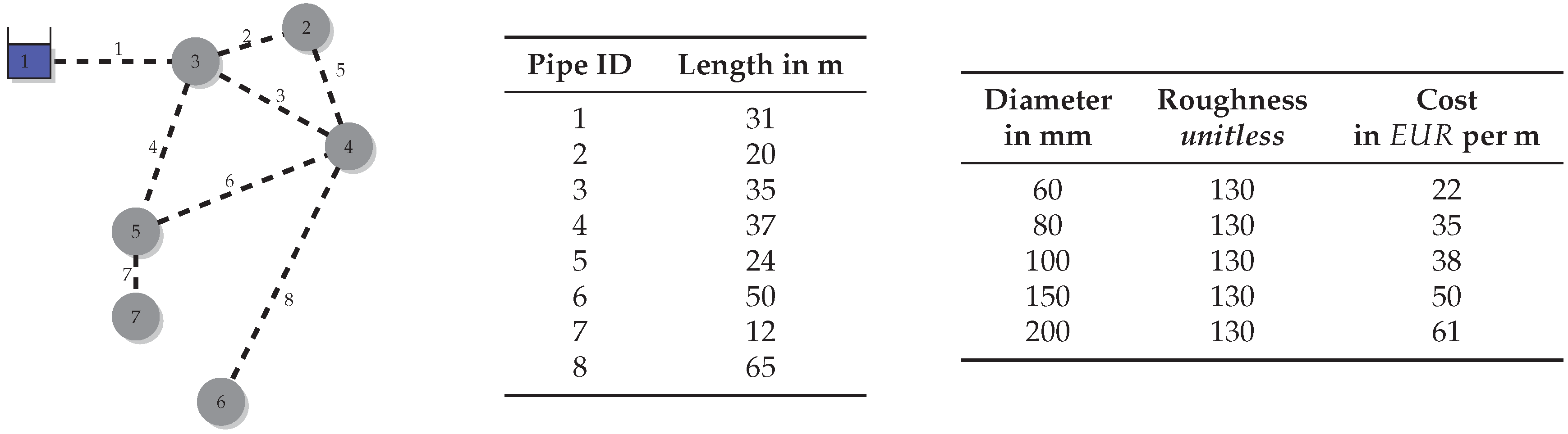
| Candidate | Pipe ID | 1 | 2 | 3 | 4 | 5 | 6 | 7 | 8 | Feasibility |
|---|---|---|---|---|---|---|---|---|---|---|
| Solution | Length (in m) | 31 | 20 | 35 | 37 | 24 | 50 | 12 | 65 | TIC |
| candidate | diameter (in mm) | 150 | 150 | 80 | 80 | 100 | 60 | 60 | 80 | feasible |
| solution 1 | cost (in ) | 1550 | 1000 | 1225 | 1295 | 912 | 1100 | 264 | 2275 | 9621 |
| candidate | diameter (in mm) | 150 | 150 | 80 | 60 | 100 | 60 | 60 | 80 | infeasible |
| solution 2 | cost (in ) | 1550 | 1000 | 1225 | 814 | 912 | 1100 | 264 | 2275 | 9140 |
| candidate | diameter (in mm) | 150 | 150 | 60 | 80 | 100 | 60 | 60 | 80 | feasible |
| solution 3 | cost (in ) | 1550 | 1000 | 770 | 1295 | 912 | 1100 | 264 | 2275 | 9166 |
| candidate | diameter (in mm) | 150 | 100 | 80 | 80 | 100 | 60 | 60 | 80 | infeasible |
| solution 4 | cost (in ) | 1550 | 760 | 770 | 1295 | 912 | 1100 | 264 | 2275 | 8926 |
| Parameter | Levels | Value |
|---|---|---|
| # Iterations | 4 | 100, 200, 300, 400 |
| # Pipes | 5 | 100, 200, 300, 400, 500 |
| Meshedness | 3 | 0.10, 0.15, 0.20 |
| Initial solution | 2 | highCost, lowCost |
| Pipe sort | 2 | lengthSort, costSort |
| Grasp size | 3 | 0%, 10%, 20% |
| Memory list | 2 | memory, noMemory |
| Perturbation rate | 5 | 1%, 10%, 20%, 30%, 40% |
| Network | Meshedness | Pipes | Demand | Water | Network | Meshedness | Pipes | Demand | Water |
|---|---|---|---|---|---|---|---|---|---|
| Coefficient | Nodes | Reservoirs | Coefficient | Nodes | Reservoirs | ||||
| HG-MP-1 | 0.20 | 100 | 73 | 1 | HG-MP-16 | 0.20 | 606 | 431 | 4 |
| HG-MP-2 | 0.15 | 100 | 78 | 1 | HG-MP-17 | 0.15 | 607 | 465 | 4 |
| HG-MP-3 | 0.10 | 99 | 83 | 1 | HG-MP-18 | 0.10 | 608 | 503 | 5 |
| HG-MP-4 | 0.20 | 198 | 143 | 1 | HG-MP-19 | 0.20 | 708 | 503 | 5 |
| HG-MP-5 | 0.15 | 200 | 155 | 1 | HG-MP-20 | 0.15 | 703 | 538 | 5 |
| HG-MP-6 | 0.10 | 198 | 166 | 1 | HG-MP-21 | 0.10 | 707 | 586 | 5 |
| HG-MP-7 | 0.20 | 299 | 215 | 2 | HG-MP-22 | 0.20 | 805 | 572 | 6 |
| HG-MP-8 | 0.15 | 300 | 232 | 2 | HG-MP-23 | 0.15 | 804 | 615 | 6 |
| HG-MP-9 | 0.10 | 295 | 247 | 2 | HG-MP-24 | 0.10 | 808 | 669 | 6 |
| HG-MP-10 | 0.20 | 397 | 285 | 2 | HG-MP-25 | 0.20 | 906 | 644 | 6 |
| HG-MP-11 | 0.15 | 399 | 308 | 2 | HG-MP-26 | 0.15 | 905 | 692 | 7 |
| HG-MP-12 | 0.10 | 395 | 330 | 3 | HG-MP-27 | 0.10 | 908 | 752 | 7 |
| HG-MP-13 | 0.20 | 498 | 357 | 2 | HG-MP-28 | 0.20 | 1,008 | 716 | 7 |
| HG-MP-14 | 0.15 | 499 | 385 | 3 | HG-MP-29 | 0.15 | 1,007 | 770 | 7 |
| HG-MP-15 | 0.10 | 495 | 413 | 3 | HG-MP-30 | 0.10 | 1,009 | 835 | 8 |
| Number | Diameter | Roughness | Cost | Number | Diameter | Roughness | Cost |
|---|---|---|---|---|---|---|---|
| (in mm) | (unitless) | (in per m) | (in mm) | (unitless) | (in per m) | ||
| 1 | 20 | 130 | 9 | 200 | 130 | 116 | |
| 2 | 30 | 130 | 20 | 10 | 250 | 130 | 150 |
| 3 | 40 | 130 | 25 | 11 | 300 | 130 | 201 |
| 4 | 50 | 130 | 30 | 12 | 350 | 130 | 246 |
| 5 | 60 | 130 | 35 | 13 | 400 | 130 | 290 |
| 6 | 80 | 130 | 38 | 14 | 500 | 130 | 351 |
| 7 | 100 | 130 | 50 | 15 | 600 | 130 | 528 |
| 8 | 150 | 130 | 61 | 16 | 1,000 | 130 | 628 |
© 2016 by the authors; licensee MDPI, Basel, Switzerland. This article is an open access article distributed under the terms and conditions of the Creative Commons Attribution (CC-BY) license (http://creativecommons.org/licenses/by/4.0/).
Share and Cite
De Corte, A.; Sörensen, K. An Iterated Local Search Algorithm for Multi-Period Water Distribution Network Design Optimization. Water 2016, 8, 359. https://doi.org/10.3390/w8080359
De Corte A, Sörensen K. An Iterated Local Search Algorithm for Multi-Period Water Distribution Network Design Optimization. Water. 2016; 8(8):359. https://doi.org/10.3390/w8080359
Chicago/Turabian StyleDe Corte, Annelies, and Kenneth Sörensen. 2016. "An Iterated Local Search Algorithm for Multi-Period Water Distribution Network Design Optimization" Water 8, no. 8: 359. https://doi.org/10.3390/w8080359