Article

Development of Field Pollutant Load Estimation Module and Linkage of QUAL2E with Watershed-Scale L-THIA ACN Model

1
Water Pollution Load Management Research Division, National Institute of Environmental Research, Seogu, Incheon 22689, Korea
2
Department of Agricultural & Biological Engineering, Purdue University, West Lafayette, IN 47907-2093, USA
3
Department of Biological and Agricultural Engineering, Texas A&M University, College Station, TX 77843, USA
4
Water Resources Research Centre, K-Water Institute, Daejeon 34350, Korea
5
Department of Regional Infrastructure Engineering, Kangwon National University, Chuncheon 24341, Korea
*
Author to whom correspondence should be addressed.
Water 2016, 8(7), 292; https://doi.org/10.3390/w8070292
Submission received: 22 April 2016 / Revised: 24 June 2016 / Accepted: 11 July 2016 / Published: 15 July 2016

Abstract

:
The Long Term Hydrologic Impact Assessment (L-THIA) model was previously improved by incorporating direct runoff lag time and baseflow. However, the improved model, called the L-THIA asymptotic curve number (ACN) model cannot simulate pollutant loads from a watershed or instream water quality. In this study, a module for calculating pollutant loads from fields and through stream networks was developed, and the L-THIA ACN model was combined with the QUAL2E model (The enhanced stream water quality model) to predict instream water quality at a watershed scale. The new model (L-THIA ACN-WQ) was applied to two watersheds within the Korean total maximum daily loads management system. To evaluate the model, simulated results of total nitrogen (TN) and total phosphorus (TP) were compared with observed water quality data collected at eight-day intervals. Between simulated and observed data for TN pollutant loads in Dalcheon A watershed, the R2 and Nash–Sutcliffe efficiency (NSE) were 0.81 and 0.79, respectively, and those for TP were 0.79 and 0.78, respectively. In the Pyungchang A watershed, the R2 and NSE were 0.66 and 0.64, respectively, for TN and both statistics were 0.66 for TP, indicating that model performed satisfactorily for both watersheds. Thus, the L-THIA ACN-WQ model can accurately simulate streamflow, instream pollutant loads, and water quality.

1. Introduction

Estimation of pollutant loads in watersheds is very important for long-term watershed management plans such as non-point source (NPS) pollution management or total maximum daily loads (TMDLs) [1]. To estimate pollutant loads at a watershed, long-term monitoring of flow and water quality is essential. However, due to limitations in monitoring flow and pollutants in terms of labor and budget [2], various computer models have been developed and used worldwide [3,4,5,6,7]. Diverse input data are needed to operate complex watershed-scale hydrology or water quality models such as SWAT (Soil and Water Assessment Tool) [8], HSPF (Hydrologic Simulation Program–Fortran) [9], and SWMM (Storm Water Management Model) [10,11]. For this reason, simpler computer models, such as PLOAD (Pollutant Loading Application) [12], STEPL (Spreadsheet Tool for Estimating Pollutant Load [13,14], and L-THIA (Long Term Hydrologic Impact Assessment) [15,16,17,18], have been used at the screening level. Among these models, L-THIA has been used in various studies and long-term watershed management plans because only daily rainfall data, in conjunction with a land use or soil dataset, are needed for daily direct runoff simulation and pollutant loads using the Natural Resources Conservation Services curve number (NRCS-CN) method and event mean concentration (EMC) databases for representative land uses [17,19,20,21]. The ArcView/ArcGIS/Web/Web GIS interface to the L-THIA model has been developed and used for almost two decades [15,16,18,20,22,23]. The Low Impact Development (LID) module was developed and integrated into L-THIA for environmentally friendly urban land use planning [24].
However, the current L-THIA model has limitations in estimating direct runoff during low-flow season because it does not compute direct runoff depending on the amount of rainfall [17,25,26]. In addition, the baseflow component for each hydrologic response unit (HRU) is not simulated [17]. When applying the L-THIA model to a watershed, lag time of the direct runoff component (to account for time needed to reach streams), the baseflow component contribution from unconfined aquifers, and flow routing through channel networks should all be considered. These limitations were addressed in the watershed-scale L-THIA asymptotic curve number (ACN) model developed by Ryu et al. [27].
With these capabilities enhanced, the watershed-scale L-THIA ACN model could be used at ungauged watersheds for streamflow estimation. However, it does not simulate pollutant loads from HRUs, or evaluate the effects of watershed routing on water quality changes through stream networks.
Thus, the objectives of this study are to (1) develop a module for estimation of pollutant loads from fields based on EMC databases for various land uses and amounts of rainfall; (2) to add the QUAL2E model (The enhanced stream water quality model) for stream water quality modeling to the watershed-based L-THIA model; and (3) to evaluate the accuracy of the watershed-scale L-THIA ACN model with water quality (watershed-scale L-THIA ACN-WQ model) by comparing estimated water quality with observed water quality.

2. Materials and Methods

2.1. Development of the Water Quality Simulation Module of the Watershed-Scale L-THIA ACN Model

The watershed-scale L-THIA ACN model, developed by Ryu et al. [27], does not include a water quality component. Therefore, a field pollutant load estimation module and a stream water quality module were added to the L-THIA model (Figure 1).
In the L-THIA model, pollutant loads for eight representative land uses were computed by multiplying EMC data collected in the USA by direct runoff volume [17,28].

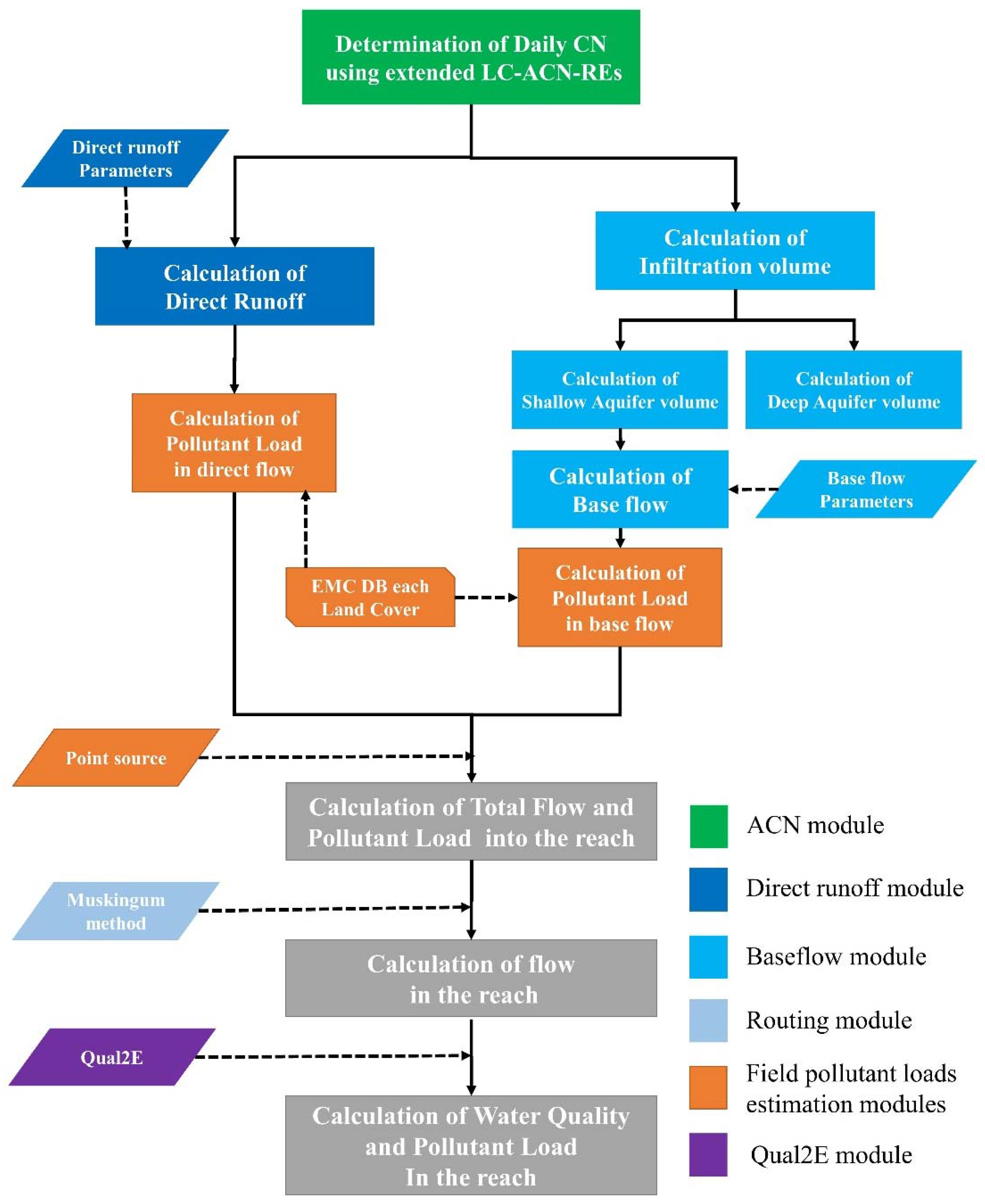
2.1.1. Development of the Field Pollutant Load Estimation Module

To develop the field pollutant load estimation module, it is assumed that pollutant loads through direct runoff and baseflow should be estimated from each HRU, and move to the stream of each subbasin. For this, the EMC data for direct runoff and baseflow components for various land cover types are needed. However, EMC data on infiltration from various land cover types are not available in South Korea, as is the case in many other countries. Thus, pollutant load from the baseflow component was estimated by multiplying the baseflow by adjusted EMC data. The adjusted EMC data is calculated by multiplying the EMC concentration by a user-defined coefficient to explain adsorption or degradation through soil and the loss of some portions to deep aquifers [29]. The EMC data were derived from monitoring data collected at various locations; thus, regional characteristics of EMC should be considered when these EMC data are applied. The EMC adjustment coefficients were used in pollutant estimation from each HRU in this study (Equation (1)), which allows ease of model use, providing reasonable accuracy using a limited number of input parameters, similar to the original L-THIA model [15,16,17,18].
E M C D R = E M C × A d j _ E M C D R E M C B F = E M C × A d j _ E M C B F
where EMCDR is the pollutant concentration in direct runoff (mg/L), EMCBF is the pollutant concentration in baseflow (mg/L), EMC is the initial pollutant concentration of both direct runoff and baseflow (mg/L), Adj_EMCDR is the adjustment coefficient for EMC in the direct runoff, and Adj_EMCBF is the adjustment coefficient for EMC in the baseflow.
The pollutant loads through either direct runoff or baseflow from each HRU (Equation (2)) are summed together for each subbasin (Equation (3)) and then these loads, later converted to concentration of pollutants, are used as input data to the instream water quality simulation (Equation (4)):
L D R , h r u = [ E M C D R × Q D R , H R U 1000 ] L B F , h r u = [ E M C B F × Q B F , H R U 1000 ]
where LDR,hru is the pollutant load of direct runoff (kg), LBF,hru is the pollutant load of baseflow (kg), EMCDR is the pollutant concentration in direct runoff (mg/L), EMCBF is the pollution concentration in baseflow (mg/L), QDR,HRU is the amount of direct runoff (m3) discharged to the main channel, and QBF,HRU the amount of baseflow (m3) into the main channel:
L D R , s u b = H R U n L D R , h r u L B F , s u b = H R U n L B F , h r u
C D R , s u b = [ L D R , s u b × 1000 Q D R , s u b ] C B F , s u b = [ L B F , s u b × 1000 Q B F , s u b ]
where LDR,sub is the pollutant load of direct runoff in subbasin (kg), LBF,sub is the pollutant load of baseflow in subbasin (kg), CDR is the pollutant concentration of direct runoff in the subbasin (mg/L), CBF is the pollutant concentration of baseflow in the subbasin (mg/L), QDR,sub is the amount of direct runoff discharged to the streams in the subbasin (m3), and QBF,sub is the amount of baseflow into the main channel in the subbasin (m3).
The EMC data from the “Project of the long-term monitoring for the nonpoint source (NPS) pollution”, monitored by the Ministry of Environment (MOE) in South Korea, were used (Table 1) because the EMC data for various land cover types and rainfall ranges are available in these datasets. The NPS pollution loads have been measured over seven years (2008–2015) in a small subbasin for thirteen representative land covers. The data compiled through this long-term monitoring project have information on NPS pollution, such as the amount and ratio of NPS pollution in runoff, and EMC data [30,31,32,33]. In recent years, the MOE of Korea has determined the EMC and unit loads for each land cover using the 7-year data from the project. The data were validated through government hearings [34].

2.1.2. Incorporation of Simplified QUAL2E Instream Water Quality Model

In this study, the simplified QUAL2E model [35], which has been widely used in one-dimensional water quality simulation, was added into the channel routing module of the watershed-scale L-THIA ACN model. The mechanism of instream water quality changes in the QUAL2E model is given in Brown and Barnwell [35].
To simulate water quality through stream networks using the simplified QUAL2E, flow and pollutant concentration parameters from each subbasin must be prepared. Pollutant concentrations calculated in Section 2.1.1 were classified as total nitrogen (TN) and total phosphorus (TP), without being further divided into specific categories such as nitrate nitrogen (NO3-N), nitrite nitrogen (NO2-N), ammonia nitrogen (NH3-N), organic nitrogen (organic-N), organic phosphorus (organic-P), and inorganic-phosphorus (inorganic-P). However, for simulation of instream water quality changes, division into these categories is required.
Thus, pollutant concentrations of TN and TP in both direct runoff and baseflow were subdivided by partitioning coefficient parameters, which must be prepared by model users based on water quality data collected in the study watershed or nearby areas. After partitioning TN and TP, the six pollutant concentrations (NO3-N, NO2-N, NH3-N, organic-N, organic-P and inorganic-P) of the subbasin, and of the direct runoff and baseflow, were used as input data for water quality simulation in streams, using the method in Brown and Barnwell [23]. For the baseflow component, organic-N and organic-P were excluded because these nutrients have greater adsorption characteristics to soil particles while moving downwards from the surface. Only soluble pollutants can infiltrate into aquifers from the land surface [29]. The QUAL2E model can only simulate carbonaceous biochemical oxygen demand (CBOD), and not bottle BOD5 (five-day biochemical oxygen demand); therefore, bottle BOD5 of the subbasin calculated by Equation (4) was converted to CBOD following Equation (5):
C B O D u = b o t t l e B O D 5 4.57 ( N H 3 ) ( 1 e 5 × k n b ) α 4 A ( 1 e 5 × ρ ) 1 e 5 × k d b
where CBODu is the ultimate CBOD concentration (mg/L), hereinafter referred as CBOD, and bottleBOD5 is the bottle BOD5 concentration calculated by Section 2.1.1 (mg/L), NH3 is the ammonia concentration (mg/L), A is the algal biomass (mg/L), ρ is the respiration rate of algae (day−1), knb is the nitrification rate coefficient in bottle BOD5 at 20 °C (day−1), and kdb is the deoxidation rate coefficient in bottle BOD5 at 20 °C (day−1).
Since initial dissolved oxygen (DO) and algae pollutant concentrations required in QUAL2E are not available in the EMC databases (Table 1), the initial concentration of DO was estimated using the method proposed by APHA (Washington, DC, USA) [36]. Changes in DO were calculated using the method in Brown and Barnwell [35]. The amount of algal biomass is closely related to chlorophyll a and can be derived by using its relationship with the concentration of chlorophyll a [37]. Chlorophyll a concentration was derived by using a simplified version of the exponential function proposed by Cluis et al. [37] (Equation (5)):
C h l = 0   ,     i f   Q D R , s u b < 10 5 m 3 / s ,   o r   ( T P   a n d   T N   <   10 6 ) C h l = 0.5 × 10 2.7 Q D R , s u b   ,     i f   Q D R , s u b > 10 5 m 3 / s ,   a n d   ( T P   a n d   T N   >   10 6 ) C h l = 0.5 × 10 0.5 Q D R , s u b   ,   i f   Q D R , s u b > 10 5 m 3 / s ,   T P < 10 6 a n d   T N > 10 6
where Chl is the chlorophyll a concentration in the direct runoff (μ/L), QDR,sub is direct runoff flow rate into the main channel (m3/s), TN is the total Kjeldahl nitrogen load (kmol), TP is the total phosphorus load (kmol).
The initial concentration of DO was estimated using Equation (7) proposed by APHA (Washington, DC, USA) [36]:
D O = exp [ 139.34410 + 1.575701 × 10 5 T e m p K 6.642308 × 10 7 T e m p K 2 + 1.243800 × 10 10 T e m p K 3 8.621949 × 10 11 T e m p K 4 ]
where DO is the saturation concentration of dissolved oxygen (mg/L), and TempK is water temperature in Kelvin (273.15 + °C).
Water temperature was calculated using Equation (8) proposed by Stefan and Preud’ homme [38]:
T e m p K = 273.15 + ( 5.0 + 0.75 T a v e r a g e )
where TempK is water temperature during the day (°C) and Taverage is the average air temperature during the day (°C).
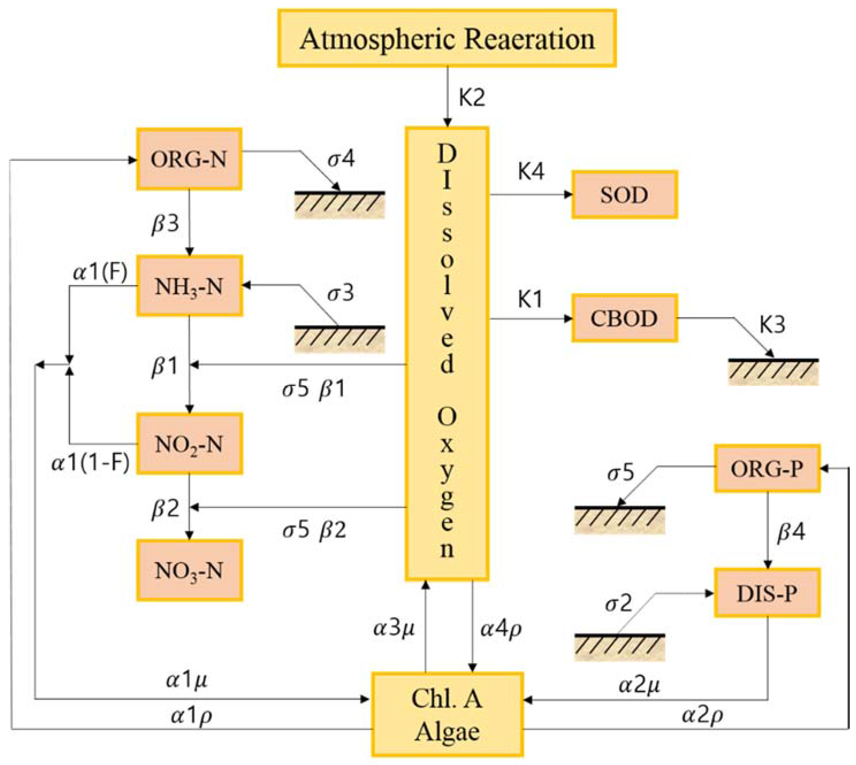
The initial concentrations of chlorophyll a and DO in the subbasin were used for input data of the instream water quality component of the watershed-scale L-THIA ACN-WQ model. The mechanism of instream water quality changes in the QUAL2E model is shown in Figure 2. More detailed description for each submodule of QUAL2E is explained below in details.
Weather data (e.g., solar radiation, duration of solar radiation and average air temperature) are required to simulate instream water quality changes using QUAL2E. A change in algae biomass in streams affects nutrient levels. The amount of algal biomass is simulated using solar radiation and duration as outlined by Brown and Barnwell [35]. The watershed-scale L-THIA ACN-WQ model was modified to use the weather data for instream water quality simulation.
In the watershed-scale L-THIA ACN-WQ model, the EMC data can be adjusted to consider local EMC characteristics. The subdivisions of TN and TP were added to the model to simulate the NO3-N, NO2-N, NH3-N, organic-P and inorganic-P in streams (Table 2).
Pollutant loads in the stream were simulated using the QUAL2E model and the parameters in QUAL2E were used in the watershed-scale L-THIA ACN-WQ model (Table 3). The default values of QUAL2E parameters were set in the model, as shown in Table 3, with reference to studies of Glavan et al. and Na [39,40].

2.2. Applications of the Watershed-Scale L-THIA ACN-WQ Model

To evaluate the watershed-scale L-THIA ACN-WQ model, estimated streamflow and pollutant loads were compared with observed data at two study watersheds (Dalcheon A and Pyungchang A in South Korea where the TMDL was carried out; Figure 3).
Dalcheon A is located in the Han River basin in South Korea. The average slope of this watershed (22.0%) is lower than that of Pyungchang A watershed (30.8%). Land cover types in Dalcheon A consist of forest (71.9%), agricultural (18.6%), urban (2.5%), bare land (0.9%) and others (6.1%).
Pyungchang A is also located in the Han-River basin. The land cover types consist of forest (80.5%), agricultural (12.8%), urban (1.7%), bare land (2.0%), and others (1.2%).
Information on the study watersheds including surface area, soil, climate, agriculture production type and water quality information are shown in Table 4.
The watershed-scale L-THIA ACN-WQ model, which can estimate instream water quality, was applied to these study watersheds for the period 2010–2014. The hydrology model parameters and water quality-related parameters were calibrated using 8-day interval observed flow and water quality data (the only flow and water quality data available for these TMDL watersheds).
In addition to the adjusted EMC, various QUAL2E parameters such as algal respiration rate, algal settling rate, algal growth rate, nitrification rate of nitrite, and phosphorus settling rate were adjusted for a better fit with measured TN and TP data, when calibrating instream water quality of TN and TP.

3. Results and Discussion

3.1. Estimation of Pollutant Load

For assessing the model performance, parameters of the model were manually calibrated by comparing model simulations with observations for streamflow, TN, and TP. Pearson coefficient of correlation (R2) and Nash–Sutcliffe simulation efficiency index (NSE) [41] were used as the objective function, all of which are well known and generally used in evaluating the performance of models [39,42].
The calibrated CN values in Dalcheon A and Pyungchang A are 3% lower and 9% higher, respectively, than the default CN values (Table 5). The calibrated value for field slope length at Dalcheon A watershed is 1.5 times greater than that estimated from the relationship between average slope and slope length suggested by Wischmeier and Smith [43].
Threshold water levels (aqfthr) in Dalcheon A and Pyungchang A were 20 mm and 30 mm, respectively.
Calibrated parameters of the watershed-scale L-THIA ACN-WQ model indicate that EMC adjustment coefficients affect instream water quality as well as pollutant loads from each subbasin (Table 6). This indicates that the EMC should be adjusted to account for differences in agricultural management (fertilizer/manure application rates, tillage, etc.) or urban impervious areas and population density at each watershed.
As shown in the calibration result, EMCs can be different for direct runoff and baseflow, and they should be separately calibrated.
In many other countries, including South Korea, it is difficult to predict the EMCs for baseflow by individual land cover type.
Therefore, if the L-THIA ACN-WQ model is calibrated with the EMC for baseflow in areas with various land cover types, the representative EMCs for baseflow by individual land cover type could be estimated. Furthermore, the representative EMCs for baseflow could be used for estimating a representative ratio of baseflow pollution loads to streamflow pollution loads that can contribute to estimating pollutant loads for baseflow in ungauged watersheds.
The parameters of the partitioning coefficients of organic N, NO3-N, and NH3-N in TN and organic-P in TP were defined based on the ratio of measured water quality data from outlets in the study watersheds (Table 6). Organic-N, NO3-N, NH3-N, and organic P (thus inorganic P) ratio values are similar in both watersheds, while NO2-N concentrations are different. Thus, these partitioning values (organic-N, NO3-N, NH3-N, and organic P) from observed data were used as model inputs for both study watersheds, while these could be adjusted or calibrated based on local flow and water quality conditions. If no observed water quality data are available, these partitioning model parameters could be calibrated to reflect local conditions indirectly. Parameters related to water quality in streams (e.g., respiration rate of algae, growth rate of algae, settling rate for phosphorus, nitrification rate) were calibrated manually to better reflect stream characteristics.

3.2. Model Performance Compared to Observed Streamflow And Pollutant Loads

Estimated average streamflow using the watershed-scale L-THIA ACN-WQ model and observed streamflow at Dalcheon A watershed were 27.68 m3/s and 26.29 m3/s, respectively. The R2 and NSE values were 0.79 and 0.78, respectively (Table 7, Figure 4). Estimated average and observed streamflow at Pyungchang A watershed were 56.48 m3/s and 53.69 m3/s, respectively (Table 7, Figure 5).
Average estimated and observed TN pollutant loads in Dalcheon A were 5227.04 kg and 6077.44 kg, respectively, (Table 8) and R2 and NSE values were 0.74 and 0.72, respectively (Figure 6). Estimated and observed pollutant loads in Pyungchang A were 10,282.49 kg and 13,457.67 kg, respectively (Table 8). The R2 and NSE values were 0.66 and 0.64, respectively (Figure 7).
Average estimated and observed TP pollutant loads in Dalcheon A were 195.75 kg and 242.13 kg, respectively. R2 and NSE values were 0.70 and 0.64. Average pollutant loads estimated and observed in Pyungchang A were 306.02 kg and 302.51 kg. The R2 and NSE values were both 0.66 (Table 8, Figure 8 and Figure 9).
The simulated and observed data for concentrations of TN and TP match reasonably well. For Dalcheon A, estimated and observed TN concentration values were 2.70 mg/L and 2.76 mg/L, respectively (Table 8). TP estimated and observed values were 0.03 mg/L and 0.02 mg/L, respectively. For Pyungchang A watershed, average simulated and observed values were 2.35 and 2.91 mg/L of TN, and 0.04 and 0.03 mg/L of TP, respectively.
These results show that the watershed-scale L-THIA ACN-WQ model can simulate not only streamflow but also pollutant loads at a watershed with less input data required than for complex watershed-scale models.

4. Conclusions

In this study, the watershed-scale L-THIA ACN model, developed by Ryu et al. [27], was enhanced by developing a field pollutant load estimation module and incorporating the instream QUAL2E model, in order to simulate pollutant loads at a watershed scale. Comparison of the simulated results of this L-THIA ACN-WQ model with observed values from two watersheds in South Korea reveal that the model can simulate not only streamflow but also pollutant loads reasonably well [44,45].
Eight parameters used for calculating pollutant loads in each land cover and 33 parameters for water quality changes in streams were added in the model. The model requires 51 parameters (ten for streamflow, eight for pollutant loads from the watershed, and 33 for instream water quality—default values for these 33 parameters, recommended by the US EPA, are available) in order to simulate streamflow and water quality.
Based on the calibrated parameters, the default values of the 33 instream water quality parameters could be used at ungagged watersheds in conjunction with ten (for streamflow) and eight (for watershed pollutant loads) model parameters prepared according to the localized conditions of the watershed in question. Further evaluations of the watershed-scale L-THIA ACN-WQ model under different weather, land use, and soil conditions are needed.
This study attempted to improve the shortcomings of the existing L-THIA model, which could simulate only pollutant loads for direct runoff. The model suggested in this study can estimate the total instream pollutant loads and water quality considering baseflow as well as direct runoff.
Furthermore, existing watershed models such as SWAT or HSPF involve complex hydrologic components and many parameters related to the watershed characteristics [46]. Consequently, users need to spend lots of time and effort to calibrate various model parameters.
On the other hand, the L-THIA ACN-WQ model can successfully estimate the total streamflow (direct runoff and baseflow) and instream pollutant loads with less parameters than those of SWAT or HSPF. In addition, the operating time of models for long-term simulations is significantly reduced when compared to the other catchment models.
In this regard, we believe that the L-THIA ACN-WQ model can be a useful tool for simulating streamflow and water quality for sustainable watershed management plans.
Nevertheless, there are still limitations in the developed model in that sensitivity and uncertainty analysis should be manually conducted. Moreover, the model has no function for simulating other water qualities (e.g., suspended soil) excluding the BOD, TN, and TP.
Thus, in the near future, an auto-calibration tool associated with various optimal-algorithms will be mounted on the model to conduct sensitivity and uncertainty analysis. Furthermore, new simple modules to simulate various water qualities such as SS and TOC will be added to the model.

Acknowledgments

This research was supported by the Geo-Advanced Innovative Action (GAIA) Project (No. 2014000540003, Surface Soil Resources Inventory & Integration: SSORII Research Group) in South Korea.

Author Contributions

Jichul Ryu wrote the paper, developed the module and combined watershed scale L-THIA ACN model and QUAL2E model; Won Seok Jang built the topography GIS data for study watersheds; Jonggun Kim applied and evaluated the model; Younghun Jung and Bernard A. Engel provided critical comments and revision of manuscript; Kyoung Jae Lim conceived the idea for the project and provided many useful suggestions to improve the analysis of the results and supervised the research.

Conflicts of Interest

The authors declare no conflict of interest.

References

  1. United States Environmental Protection Agency (USEPA). National Management Measures to Control Nonpoint Source Pollution from Agriculture; EPA 841-B-03-004; U.S. Environmental Protection Agency Office of Water (4503T): Washington, DC, USA, 2003.
  2. Holvoet, K.M.; Seuntjens, P.; Vanrolleghem, P.A. Monitoring and modeling pesticide fate in surface waters at the catchment scale. Ecol. Model. 2007, 209, 53–64. [Google Scholar] [CrossRef]
  3. Jeon, J.H.; Yoon, C.G.; Donigian, A.S.; Jung, K.W. Development of the HSPF-Paddy model to estimate watershed pollutant loads in paddy farming regions. Agric. Water Manag. 2007, 90, 75–86. [Google Scholar] [CrossRef]
  4. Li, Z.; Luo, C.; Xi, Q.; Li, H.; Pan, J.; Zhou, Q.; Xiong, Z. Assessment of the AnnAGNPS model in simulating runoff and nutrients in a typical small watershed in the Taihu Lake basin, China. Catena 2015, 133, 349–361. [Google Scholar] [CrossRef]
  5. Ribarova, I.; Ninov, P.; Cooper, D. Modeling nutrient pollution during a first flood event using HSPF software: Iskar River case study, Bulgaria. Ecol. Model. 2008, 211, 241–246. [Google Scholar] [CrossRef]
  6. Ryu, J.; Cho, J.; Kim, I.J.; Mun, Y.; Moon, J.P.; Kim, N.W.; Lim, K.J. Enhancement of SWAT-REMM to simulate reduction of total nitrogen with riparian buffer. Trans. ASABE 2011, 54, 1791–1798. [Google Scholar] [CrossRef]
  7. Yang, G.; Best, E.P. Spatial optimization of watershed management practices for nitrogen load reduction using a modeling-optimization framework. J. Environ. Manag. 2015, 161, 252–260. [Google Scholar] [CrossRef] [PubMed]
  8. Arnold, J.G.; Moriasi, D.N.; Gassman, P.W.; Abbaspour, K.C.; White, M.J.; Srinivasan, R.; Santhi, C.; Harmel, R.D.; van Griensven, A.; Van Liew, M.W.; et al. SWAT: Model use, calibration and validation. Trans. ASABE 2012, 55, 1491–1508. [Google Scholar] [CrossRef]
  9. Bicknell, B.; Imhoff, J.; Kittle, J.; Jobes, T.; Donigian, A. HSPF, User’s Manual; Version 12; U.S. Environmental Protection Agency: Athens, GA, USA, 2001; pp. 120–128.
  10. Gironas, J.; Roesner, L.A.; Rossman, L.A.; Davis, J. A new applications manual for the Storm Water Management Model (SWMM). Environ. Model. Softw. 2010, 25, 813–814. [Google Scholar] [CrossRef]
  11. U.S. Environmental Protection Agency (USEPA). SWMM 5 User’s Manual; EPA/600/R-05/040; National Risk Management Research Laboratory, Office of research and Development: Cincinnati, OH, USA, 2010.
  12. Edwards, C.; Miller, M. PLOAD Version 3.0 User’s Manual; United States Environmental Protection Agency (USEPA): Washington, DC, USA, 2001.
  13. Tetra Tech, Inc. User’s Guide Spreadsheet Tool for the Estimation of Pollutant Load (STEPL); Version 4.1; Tetra Tech, Inc.: Fairfax, VA, USA, 2011. [Google Scholar]
  14. Park, Y.S.; Engel, B.A.; Harbor, J. A web-based model to estimate the impact of best management practices. Water 2014, 6, 455–471. [Google Scholar] [CrossRef]
  15. Bhaduri, B.; Grove, M.; Lowry, C.; Harbor, J. Assessing the long-term hydrologic impact of land-use change: Cuppy McClure watershed, Indiana. J. Am. Water Works Assoc. 1997, 89, 94–106. [Google Scholar]
  16. Engel, B.A. GIS-based CN Runoff Estimation; Agricultural and Biological Engineering Departmental Report; Purdue University: West Lafayette, IN, USA, 1997. [Google Scholar]
  17. Harbor, J.M. A practical method for estimating the impact of land-use change on surface runoff, groundwater recharge and wetland hydrology. J. Am. Plan. Assoc. 1994, 60, 95–108. [Google Scholar] [CrossRef]
  18. Lim, K.J.; Engel, B.A.; Tang, Z.; Muthukrishnan, S.; Choi, J.; Kim, K. Effects of calibration on L-THIA GIS runoff and pollutant estimation. J. Environ. Manag. 2006, 78, 35–43. [Google Scholar] [CrossRef] [PubMed]
  19. Jang, C.H.; Kum, D.H.; Jung, Y.; Kim, K.; Shin, D.S.; Engel, B.A.; Shin, Y.; Lim, K.J. Development of a Web-based L-THIA 2012 direct runoff and pollutant Auto-calibration module using a genetic algorithm. Water 2013, 5, 1952–1963. [Google Scholar] [CrossRef]
  20. Lim, K.J.; Engel, B.A.; Bhaduri, B.; Harbor, J. Development of the Long Term Hydrologic Impact Assessment Tool (L-THIA) WWW System. In Proceedings of the 10th International Soil and Conservation Organization Meeting, West Lafayette, IN, USA, 24–29 May 1999; pp. 1018–1023.
  21. Ryu, J.; Kim, E.J.; Han, M.D.; Kim, Y.S.; Kum, D.H.; Lim, K.J.; Park, B.K. Enhancement of Estimation Method on the Land T-P Pollutant Load in TMDLs Using L-THIA. J. Korean Soc. Environ. Eng. 2014, 36, 162–171. [Google Scholar] [CrossRef]
  22. Jang, J.H.; Jung, K.W.; Yoon, C.G. Modification of SWAT model for simulation of organic matter in Korean watersheds. Water Sci. Technol. 2012, 66, 2355–2362. [Google Scholar] [CrossRef] [PubMed]
  23. Tang, Z.; Engel, B.A.; Lim, K.J.; Pijanowski, B.C.; Habor, J. Minimizing the Impact of urbanization on long term runoff. J. Am. Water Resour. Assoc. 2005, 41, 1347–1359. [Google Scholar] [CrossRef]
  24. Ahiablame, L.M.; Engel, B.A.; Chaubey, I. Representation and evaluation of low impact development practices with L-THIA-LID: An example for site planning. Environ. Pollut. 2012, 1, 1–13. [Google Scholar] [CrossRef]
  25. Hawkins, R.H. Asymptotic determination of runoff curve numbers from data. J. Irrig. Drain. Eng. 1993, 119, 334–345. [Google Scholar] [CrossRef]
  26. Ryu, J.; Jung, Y.; Kong, D.S.; Park, B.K.; Kim, Y.S.; Engel, B.A.; Lim, K.J. Approach of Land Cover based Asymptotic Curve Number Regression Equation to Estimate Runoff. J. Irrig. Drain. Eng. 2016, in press. [Google Scholar]
  27. Ryu, J.; Jang, W.S.; Kim, J.; Choi, J.D.; Engel, B.A.; Lim, K.J. Development of Watershed-scale Long term Hydrologic Impact Assessment Model with Asymptotic Curve Number Regression Equation. Water 2016, 8, 153. [Google Scholar] [CrossRef]
  28. Bhaduri, B.A. GIS-Based Model to Assess the Long-Term Impacts of Land Use Change on Hydrology and Nonpoint Source Pollution. Ph.D. Thesis, Purdue University, West Lafayette, IN, USA, 1998. [Google Scholar]
  29. Choi, J.D. Effect of Agricultural Activities Farm Environment of Groundwater Quality; DAESAN Agriculture Foundation: Seoul, Korea, 1995; pp. 434–444. [Google Scholar]
  30. Han River Watershed Management Committee (HRWMC). Research on Long Term Monitoring for the Non-point Source Discharge in Han River Basin; National Institute Environmental Research (NIER): Incheon, Korea, 2014. [Google Scholar]
  31. Nakdong River Basin Management Committee (GRBMC). A Monitoring and Management Scheme for the Non-Point Sources in Nakdong River Basin; National Institute Environmental Research (NIER): Incheon, Korea, 2004. [Google Scholar]
  32. Geum River Basin Management Committee (GRBMC). A Monitoring and Management Scheme for the Non-Point Sources in Geum River Basin; National Institute Environmental Research (NIER): Incheon, Korea, 2014. [Google Scholar]
  33. Youngsan River Basin Management Committee (GRBMC). A Monitoring and Management Scheme for the Non-Point Sources in Youngsan River Basin; National Institute Environmental Research (NIER): Incheon, Korea, 2014. [Google Scholar]
  34. National Institute Environmental Research (NIER). Public Hearing of Nonpoint Source Pollution Unit Load Survey; National Institute Environmental Research (NIER): Incheon, Korea, 2014. [Google Scholar]
  35. Brown, L.C.; Barnwell, T.O. The Enhanced Water Quality Models QUAL2E and QUAL2E-UNCAS Documentation and User Manual; EPA/600/3-87/007; United States Environmental Protection Agency (USEPA): Athens, GA, USA, 1987.
  36. American Public Health Association (APHA). Standard Methods for the Examination of Water and Wastewater, 16th ed.; American Public Health Association, Inc.: Washington, DC, USA, 1985. [Google Scholar]
  37. Cluis, D.; Couture, P.; Begin, R.; Visser, S.A. Potential eutrophication assessment in rivers; relationship between produced and exported loads. Swiss J. Hydrol. 1988, 50, 166–181. [Google Scholar] [CrossRef]
  38. Stefan, H.G.; Preud’Homme, E.B. Stream temperature estimation from air temperatuer. J. Am. Water Resour. Assoc. 1993, 29, 27–45. [Google Scholar] [CrossRef]
  39. Glavan, M.; Milicic, V.; Pintar, M. Finding options to improve catchment water quality Lessons learned from historical land use situations in a Mediterranean catchment in Slovenia. Ecol. Model. 2013, 261, 58–73. [Google Scholar] [CrossRef]
  40. Na, J.S. Effects of Non-Point Pollutant Sources Using QUAL2E Model. Master’s Thesis, Chosoen University, Gwang-ju, Korea, 2015. [Google Scholar]
  41. Nash, J.E.; Sutcliffe, J.V. River flow forecasting through conceptual models, Part I—A discussion of principles. J. Hydrol. 1970, 10, 282–290. [Google Scholar] [CrossRef]
  42. Glavan, M.; White, S.M.; Holman, I.P. Water quality targets and maintenance of valued landscape character—Experience in the Axe catchment, UK. J. Environ. Manag. 2012, 103, 142–153. [Google Scholar] [CrossRef] [PubMed]
  43. Wischmeier, W.H.; Smith, D.D. Predicting Rainfall Erosion Losses: A Guide to Conservation Planning; USDA Agricultural Handbook No. 537; U.S. Government Printing Office: Washington, DC, USA, 1978.
  44. Moriasi, D.N.; Arnold, J.G.; VanLiew, M.W.; Bingner, R.L.; Hrmel, R.D.; Veith, T.L. Model evaluation guidelines for systematic quantification of accuracy in watershed simulations. Trans. ASABE 2007, 50, 885–900. [Google Scholar] [CrossRef]
  45. Ramanarayanan, T.S.; Williams, J.R.; Dugas, W.A.; Hauck, L.M.; McFarland, A.M.S. Using APEX to Identify Alternative Practices for Animal Waste Management. In Proceedings of the American Society of Agricultural Engineers Annual International Meeting, Minneapolis, MN, USA, 10–14 August 1997.
  46. Duda, P.B.; Hummel, P.R.; Donigian, A.S., Jr.; Imhoff, J.C. BASINS/HSPF: Model use, calibration, and validation. Trans. ASABE 2012, 55, 1523–1547. [Google Scholar] [CrossRef]
Figure 1. Flow diagram for development of watershed-scale L-THIA ACN-WQ (Long Term Hydrologic Impact Assessment Asymptotic Curve Number-Water Quality) model.
Water 08 00292 g001
Figure 2. General structure of QUAL2E [35].
Water 08 00292 g002
Figure 3. Two study watersheds used for evaluation of watershed-scale L-THIA ACN-WQ model.
Water 08 00292 g003
Figure 4. Comparison between simulated streamflow (a) and observed streamflow (b) at Dalcheon A watershed (2011–2014).
Water 08 00292 g004
Figure 5. Comparison between simulated streamflow (a) and observed streamflow (b) at Pyungchang A watershed (2011–2014).
Water 08 00292 g005
Figure 6. Comparison between simulated TN (a) and observed TN (b) at Dalcheon A watershed (2011–2014).
Water 08 00292 g006
Figure 7. Comparison between simulated TN (a) and observed TN (b) at Pyungchang A watershed (2011–2014).
Water 08 00292 g007aWater 08 00292 g007b
Figure 8. Comparison between simulated and observed TP at Dalcheon A watershed (2011–2014).
Water 08 00292 g008
Figure 9. Comparison between simulated and observed TP at Pyungchang A watershed (2011–2014).
Water 08 00292 g009
Table 1. Monitored event mean concentration (mg/L) of individual land cover for various rainfall magnitudes.
Land CoverBOD5 (Biocheminal Oxygen Demand)TN (Total Nitrogen)TP (Total Phosphorous)
<10 mm10–3031–50>50 mm<10 mm10–3031–50>50 mm<10 mm10–3031–50>50 mm
Residential area6.486.664.663.085.445.713.174.060.3730.2890.2100.282
Manufacturing area24.9622.3610.724.973.113.497.092.940.3420.4230.3380.358
Regional public facility area32.2149.5222.7014.527.148.626.082.470.8230.7570.4250.287
Recreational facility area18.5310.7610.216.386.283.694.891.670.8450.3520.4600.269
Road10.617.178.893.316.182.682.762.010.2210.2310.2170.176
Commercial area6.528.124.484.125.815.122.595.680.2770.3310.2120.453
Upland2.263.403.573.502.382.832.332.410.2150.3860.3010.436
Orchard0.000.685.1111.370.001.936.756.890.0000.6921.3582.233
Green house4.777.136.345.781.883.045.183.120.5851.1552.9482.595
Paddy0.001.102.092.630.001.413.885.540.0000.1540.4230.962
Pasture1.181.161.221.641.332.262.482.810.0430.0590.0460.061
Forest3.805.013.463.231.692.692.303.330.1930.3250.2320.372
Bare land6.528.124.484.125.815.122.595.680.2770.3310.2120.453
Table 2. Description of event mean concentration (EMC), nitrogen, and phosphorus parameters used in instream water quality module.
Parameter NameDescriptionRangeDefault Value
Adj_EMCDR,NConstant value for adjustment of nitrogen in surface−0.9–0.91.0
Adj_EMCBF,NConstant value for adjustment of nitrogen in aquifer−0.9–0.91.0
Adj_EMCDR,PConstant value for adjustment of phosphorus in surface−0.9–0.91.0
Adj_EMCBF,PConstant value for adjustment of phosphorus in aquifer−0.9–0.91.0
TN_ratio1 1Ratio of organic-N in total nitrogen0.0–0.90.05
TN_ratio2 1Ratio of NO3-N in total nitrogen0.0–0.90.8
TN_ratio3 1Ratio of NH3-N in total nitrogen0.0–0.90.1
TP_ratio1 2Ratio of organic-P in total phosphorus0.0–0.90.5
Notes: 1 Ratio of NO2-N = 1 − (Sum of TN_ratio1, TN_ratio2 and TN_ratio3); 2 Ratio of dissolved P = 1 − TP_ratio1.
Table 3. Description of QUAL2E parameters used in instream water quality module.
Parameter NameDescriptionRecommended Range in QUAL2EDefault Value
RS1Local algal settling rate in the reach at 20 °C0.15–1.820.3408
RS2Benthic source rate for dissolved phosphorus in the reach at 20 °C0.001–0.10.1
RS3Benthic source rate for NH4-N in the reach at 20 °C0.0–1.00.0
RS4Rate coefficient for organic nitrogen settling in the reach at 20 °C0.001–0.10.001
RS5Organic phosphorus settling rate in the reach at 20 °C0.001–0.10.08
RK1Carbonaceous biological oxygen demand (CBOD) deoxygenation rate coefficient in the reach at 20 °C0.02–3.40.3
RK2Oxygen reaeration rate in accordance with Fickian diffusion in the reach at 20 °C0.0–100.01.0
RK3Rate of loss of CBOD due to settling in the reach at 20 °C−0.36–0.36−0.36
RK4Benthic oxygen demand rate in the reach at 20 °C0.0–100.00.0
BC1Rate constant for biological oxidation of NH4 to NO2 in the reach at 20 °C0.1–10.1
BC2Rate constant for biological oxidation of NO2 to NO3 in the reach at 20 °C0.2–20.2
BC3Rate constant for hydrolysis of organic N to NH4 in the reach at 20 °C0.2–0.40.03
BC4Rate constant for mineralization of organic P to dissolved P in the reach at 20 °C0.01–0.70.1
RTHAlgal respiration rate at 20 °C0.05–5.00.05
TFACFraction of photosynthetically active solar radiation0.0–1.00
MMXMaximum specific algal growth rate at 20 °C1.0–3.01.0
IGQUAL2E algae growth limiting option (1: multiplicative, 2: limiting nutrient, 3: harmonic mean)1, 2, 31
A0Ratio of chlorophyll-a to algal biomass10.0–100.010
A1Fraction of nitrogen algal biomass0.07–0.090.071
A2Fraction of phosphorus algal biomass0.01–0.020.003
A3Rate of oxygen production per unit of algal photosynthesis1.4–2.31.4
A4Rate of oxygen uptake per unit of algal respiration1.6–2.31.6
A5Rate of oxygen uptake per unit NH3-N oxidation3.0–4.03.0
A6Rate of oxygen uptake per unit NO2-N oxidation1.0–1.141.0
Lam0Non-algal portion of the light extinction coefficient0–100
Lam1Linear algal self-shading coefficient0.006–0.0650.006
Lam2Nonlinear algal self-shading coefficient0–10
KNMichaelis-Menten nitrogen half-saturation constant0.01–0.30.01
KPMichaelis-Menten phosphorus half-saturation constant0.001–0.050.001
KLLight half-saturation coefficient0.223–1.1350.223
KnbNitrification rate coefficient in CBOD50.5
KdbDeoxidation rate coefficient in CBOD50.5
PNPreference factor for ammonium nitrogen0.0–1.00.0
Table 4. Information of the study area.
Information of Study AreaDalcheon APyungchang A
Surface area (km2)1200.331756.87
Average precipitation (2011–2014) (mm/year)1315.61389.6
Average temperature (2011–2014) (degree)11.712.8
Hydrologic soil group (%)A11.811.7
B16.015.9
C36.635.8
D35.636.6
Agriculture production type (%)Upland crop42.532.6
Green house14.720.7
Ochard21.622.6
Paddy21.224.1
Average water quality (2011–2014) (mg/L)BOD0.960.88
TN2.762.91
TP0.020.03
Table 5. Calibration parameters for streamflow component of the L-THIA ACN-WQ model.
WatershedAdj_CN 1SLSUB 2DRlag 3αBF 4aqfthr 5Frconf 6BFdelay 7Mk1 8Mk2 9Mkx 10
Dalcheon A0.031.540.720.00.1010.050.950.2
Pyungchang A0.091.080.530.00.0550.250.750.5
Notes: 1 Adjusted coefficient for CN; 2 Adjustment for slope length; 3 Direct runoff lag coefficient; 4 Baseflow recession constant; 5 Threshold water level for baseflow contribution in the unconfined aquifer (mm); 6 Fraction of water flowing into confined aquifer; 7 Delay time in aquifer recharge following water infiltration at surface (day); 8 Weighting factor for influence of normal flow on storage time constant value; 9 Weighting factor for influence of low flow on storage time constant value; 10 Weighting factor for Muskingum method.
Table 6. Calibration parameters for the water quality component of the L-THIA ACN-WQ model.
ParametersDalcheon APyungchang A
Adj_EMCDR,N0.800.70
Adj_EMCBF,N0.900.90
Adj_EMCDR,P0.600.40
Adj_EMCBF,P0.400.35
TN_ratio10.030.03
TN_ratio20.950.95
TN_ratio30.010.01
TP_ratio10.400.40
RS11.001.00
RS20.0010.001
RS30.0010.01
RS40.100.001
RS50.100.1
RS62.502.50
RK10.500.50
RK25050
RK30.360.36
RK42.002.00
RK52.002.00
RK61.711.71
BC10.100.55
BC20.202.00
BC30.020.4
BC40.010.01
TFAC0.300.30
MMX11
IG33
A08080
A10.090.09
A20.010.01
A31.601.60
A422
A53.503.50
A61.001.00
Lam011
Lam10.030.03
Lam20.0540.054
KN0.750.02
KP0.0200.025
KL0.0250.75
Knb0.500.03
Kdb0.030.045
PN0.450.50
Table 7. Comparison between estimated and observed eight-day average streamflow in the period between 2011 and 2014.
WatershedAverage Streamflow (2011–2014) (m3/s)R2NSE
ObservationEstimation
Dalcheon A26.2927.680.790.78
Pyungchang A53.6956.480.760.76
Table 8. Comparison between estimated and observed eight-day average pollutant loads in the period between 2011 and 2014.
WatershedPollutant LoadsAverage Pollutant Load (2011–2014) (kg)R2NSEAverage Concentration (2011–2014) (mg/L)
ObservationEstimationObservationEstimation
Dalcheon ATN6077.445227.040.810.792.762.70
TP242.13195.750.790.780.020.03
Pyungchang ATN134,57.6710,282.490.660.642.912.35
TP302.51306.020.660.660.030.04

