
Rationalization of Altitudinal Precipitation Profiles in a Data-Scarce Glacierized Watershed Simulation in the Karakoram


Abstract
:1. Introduction
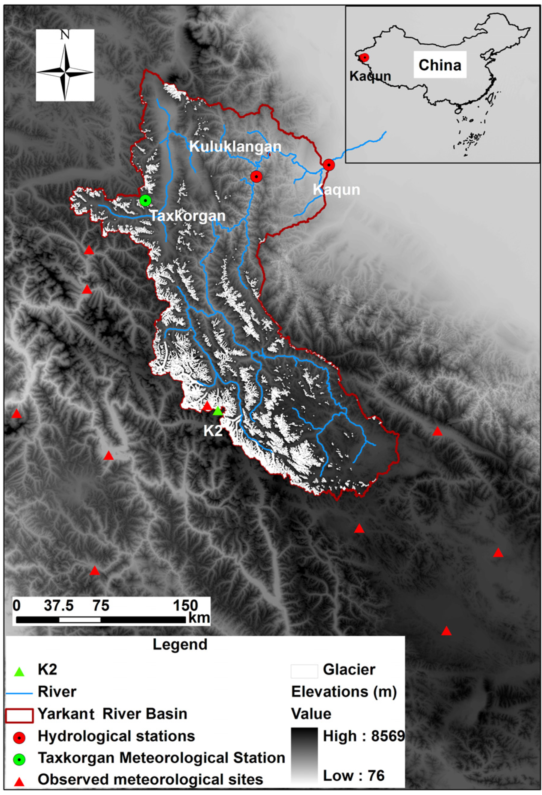
2. Study Area
3. Data and Methods
3.1. Description of the Data
3.1.1. Topography, Soil, Land Cover and Glacier Maps
3.1.2. Precipitation and Temperature
3.1.3. Observed Streamflow Data
3.2. The Glacier-Enhanced SWAT Model
3.3. Method for Rationalizing High-Elevation Precipitation
3.3.1. The Glacier Mass Accumulation-Summer Temperature Relationship
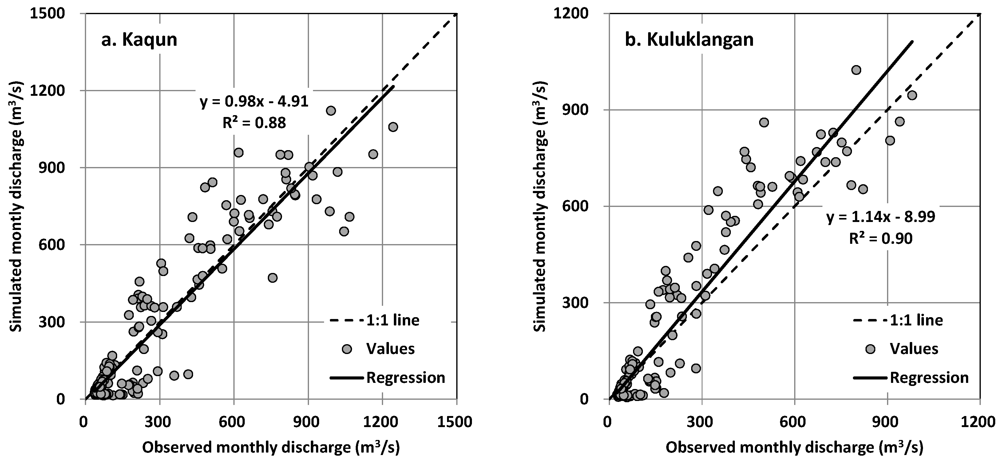
3.3.2. Calibration and Validation
3.4. Trend Analysis Method
4. Results
4.1. Parameter Setting
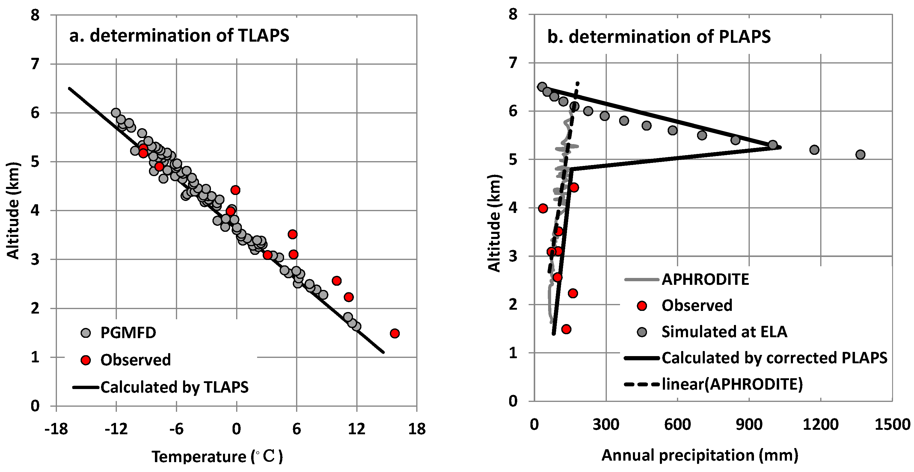
4.1.1. TLAPS
4.1.2. Other Key Model Parameters
4.2. Reconciling High-Elevation Precipitation
4.2.1. Assessment of APHRODITE Precipitation
4.2.2. Determination of PLAPS
4.2.3. Inversely Calculating Precipitation Using the Corrected PLAPS
5. Discussion
5.1. Uncertainties of the PLAPS
5.2. Explanation of Current Glacier Changes
5.2.1. Intra-Annual Distribution
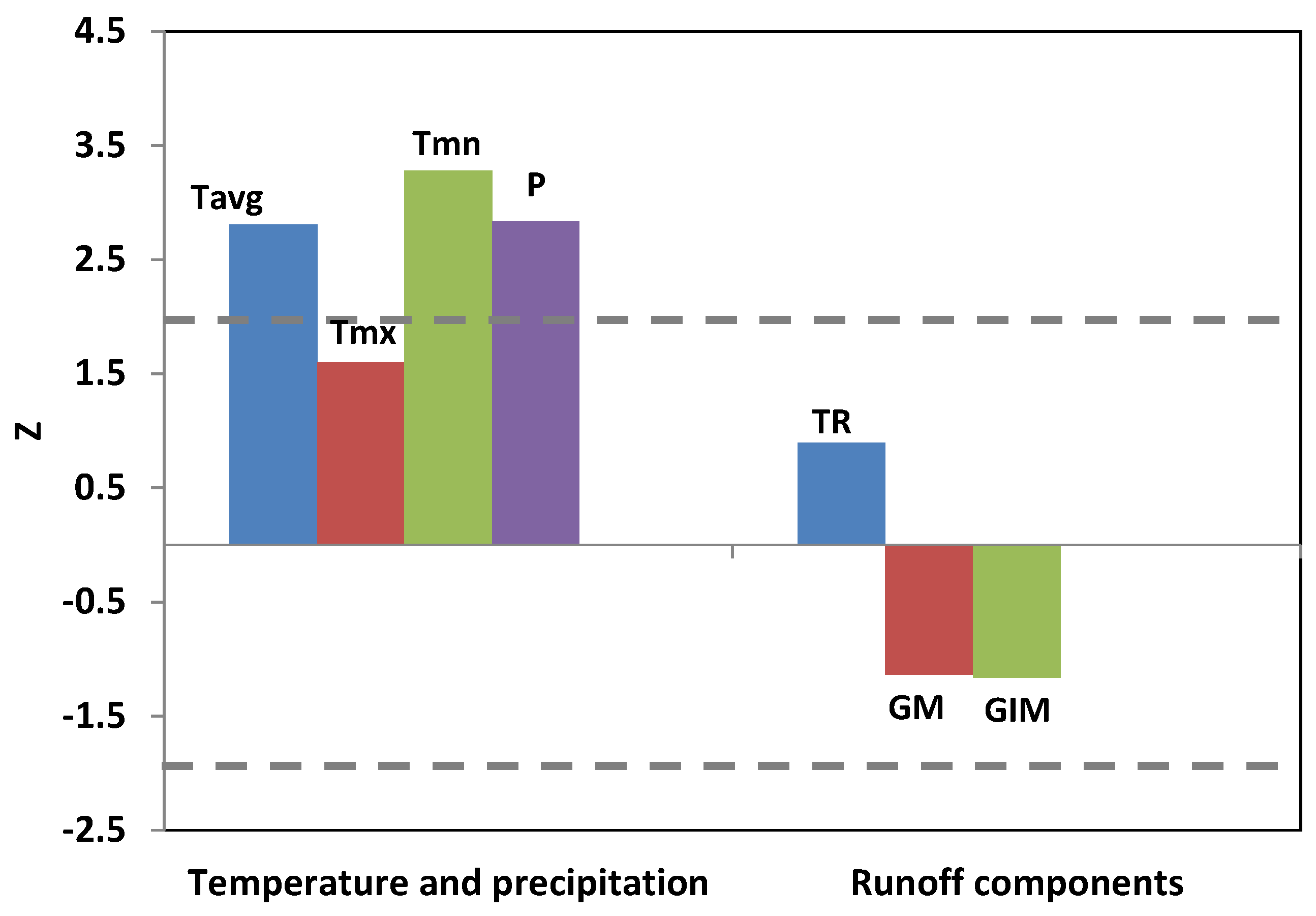
5.2.2. Trend Analysis
5.2.3. Regional Differentiation in the Karakoram
6. Conclusions
Acknowledgments
Author Contributions
Conflicts of Interest
References
- Hewitt, K. The Karakoram anomaly? Glacier expansion and the ‘elevation effect’, Karakoram Himalaya. Mt. Res. Dev. 2005, 25, 332–340. [Google Scholar] [CrossRef]
- Bolch, T.; Kulkarni, A.; Kaab, A.; Huggel, C.; Paul, F.; Cogley, J.G.; Frey, H.; Kargel, J.S.; Fujita, K.; Scheel, M.; et al. The state and fate of Himalayan glaciers. Science 2012, 336, 310–314. [Google Scholar] [CrossRef] [PubMed] [Green Version]
- Baral, P.; Kayastha, R.B.; Immerzeel, W.W.; Pradhananga, N.S.; Bhattarai, B.C.; Shahi, S.; Galos, S.; Springer, C.; Joshi, S.P.; Mool, P.K. Preliminary results of mass-balance observations of Yala glacier and analysis of temperature and precipitation gradients in Langtang valley, Nepal. Ann. Glaciol. 2014, 55, 9–14. [Google Scholar] [CrossRef]
- Unger-Shayesteh, K.; Vorogushyn, S.; Farinotti, D.; Gafurov, A.; Duethmann, D.; Mandychev, A.; Merz, B. What do we know about past changes in the water cycle of central Asian headwaters? A review. Glob. Planet. Chang. 2013, 110, 4–25. [Google Scholar] [CrossRef]
- Immerzeel, W.W.; Pellicciotti, F.; Bierkens, M.F.P. Rising river flows throughout the twenty-first century in two Himalayan Glacierized watersheds. Nat. Geosci. 2013, 6, 742–745. [Google Scholar] [CrossRef]
- Lutz, A.F.; Immerzeel, W.W.; Shrestha, A.B.; Bierkens, M.F.P. Consistent increase in high Asia’s runoff due to increasing glacier melt and precipitation. Nat. Clim. Chang. 2014, 4, 587–592. [Google Scholar] [CrossRef]
- Hagg, W.; Mayer, C.; Lambrecht, A.; Kriegel, D.; Azizov, E. Glacier changes in the big Naryn basin, central Tian Shan. Glob. Planet. Chang. 2013, 110, 40–50. [Google Scholar] [CrossRef]
- Hagg, W.; Hoelzle, M.; Wagner, S.; Mayr, E.; Klose, Z. Glacier and runoff changes in the Rukhk catchment, upper Amu-Darya basin until 2050. Glob. Planet. Chang. 2013, 110, 62–73. [Google Scholar] [CrossRef]
- Immerzeel, W.W.; Petersen, L.; Ragettli, S.; Pellicciotti, F. The importance of observed gradients of air temperature and precipitation for modeling runoff from a glacierized watershed in the Nepalese Himalayas. Water Resour. Res. 2014, 50, 2212–2226. [Google Scholar] [CrossRef]
- Yang, K.; Ye, B.S.; Zhou, D.G.; Wu, B.Y.; Foken, T.; Qin, J.; Zhou, Z.Y. Response of hydrological cycle to recent climate changes in the Tibetan plateau. Clim. Chang. 2011, 109, 517–534. [Google Scholar] [CrossRef]
- Richard, C.; Gratton, D.J. The importance of the air temperature variable for the snowmelt runoff modelling using the SRM. Hydrol. Process. 2001, 15, 3357–3370. [Google Scholar] [CrossRef]
- Petersen, L.; Pellicciotti, F. Spatial and temporal variability of air temperature on a melting glacier: Atmospheric controls, extrapolation methods and their effect on melt modeling, Juncal Norte glacier, Chile. J. Geophys. Res. Atmos. 2011, 116. [Google Scholar] [CrossRef]
- Immerzeel, W.W.; Pellicciotti, F.; Shrestha, A.B. Glaciers as a proxy to quantify the spatial distribution of precipitation in the Hunza basin. Mt. Res. Dev. 2012, 32, 30–38. [Google Scholar] [CrossRef]
- Hock, R. Glacier melt: A review of processes and their modelling. Prog. Phys. Geogr. 2005, 29, 362–391. [Google Scholar] [CrossRef]
- Garen, D.C.; Marks, D. Spatially distributed energy balance snowmelt modelling in a mountainous river basin: Estimation of meteorological inputs and verification of model results. J. Hydrol. 2005, 315, 126–153. [Google Scholar] [CrossRef]
- Kattel, D.B.; Yao, T.; Yang, K.; Tian, L.; Yang, G.; Joswiak, D. Temperature lapse rate in complex mountain terrain on the southern slope of the central Himalayas. Theor. Appl. Climatol. 2013, 113, 671–682. [Google Scholar] [CrossRef]
- Salerno, F.; Guyennon, N.; Thakuri, S.; Viviano, G.; Romano, E.; Vuillermoz, E.; Cristofanelli, P.; Stocchi, P.; Agrillo, G.; Ma, Y. Weak precipitation, warm winters and springs impact glaciers of south slopes of MT. Everest (central Himalaya) in the last 2 decades (1994–2013). Cryosphere 2015, 9, 5911–5959. [Google Scholar] [CrossRef]
- Tustison, B.; Harris, D.; Foufoula-Georgiou, E. Scale issues in verification of precipitation forecasts. J. Geophys. Res. Atmos. 2001, 106, 11775–11784. [Google Scholar] [CrossRef]
- Bookhagen, B.; Burbank, D.W. Topography, relief, and trmm-derived rainfall variations along the Himalaya. Geophys. Res. Lett. 2006, 33. [Google Scholar] [CrossRef]
- Immerzeel, W.W.; Wanders, N.; Lutz, A.F.; Shea, J.M.; Bierkens, M.F.P. Reconciling high-altitude precipitation in the upper Indus basin with glacier mass balances and runoff. Hydrol. Earth Syst. Sci. 2015, 19, 4673–4687. [Google Scholar] [CrossRef]
- Pellicciotti, F.; Buergi, C.; Immerzeel, W.W.; Konz, M.; Shrestha, A.B. Challenges and uncertainties in hydrological modeling of remote Hindu kush-karakoram-himalayan (HKH) basins: Suggestions for calibration strategies. Mt. Res. Dev. 2012, 32, 39–50. [Google Scholar] [CrossRef]
- Schaefli, B.; Hingray, B.; Niggli, M.; Musy, A. A conceptual glacio-hydrological model for high mountainous catchments. Hydrol. Earth Syst. Sci. 2005, 9, 95–109. [Google Scholar] [CrossRef]
- Valéry, A.; Andréassian, V.; Perrin, C. Regionalization of precipitation and air temperature over high-altitude catchments—Learning from outliers. Hydrol. Sci. J. 2010, 55, 928–940. [Google Scholar] [CrossRef]
- Yang, Z. Glacier Water Resources in China; Gansu Science and Technology Press: Lanzhou, China, 1991. (In Chinese) [Google Scholar]
- Chen, Y.N.; Xu, C.C.; Chen, Y.P.; Li, W.H.; Liu, J.S. Response of glacial-lake outburst floods to climate change in the Yarkant river basin on northern slope of Karakoram mountains, China. Quat. Int. 2010, 226, 75–81. [Google Scholar] [CrossRef]
- Zhang, S.Q.; Gao, X.; Ye, B.S.; Zhang, X.W.; Hagemann, S. A modified monthly degree-day model for evaluating glacier runoff changes in China. Part II: Application. Hydrol. Process. 2012, 26, 1697–1706. [Google Scholar] [CrossRef]
- Wu, L.; Li, X. Dataset of the first glacier inventory in China. Cold Arid Reg. Sci. Data Center Lanzhou 2004. [Google Scholar] [CrossRef]
- Guo, W.Q.; Xu, J.L.; Liu, S.Y.; Shangguan, D.H.; Wu, L.Z.; Yao, X.J.; Zhao, J.D.; Liu, Q.; Jiang, Z.L.; Li, P.; et al. The second glacier inventory dataset of China (version 1.0). Cold Arid Reg. Sci. Data Center Lanzhou 2014. [Google Scholar] [CrossRef]
- Frauenfelder, R.; Kääb, A. Glacier mapping from multitemporal optical remote sensing data within the Brahmaputra river basin. In Proceedings of the 33rd International Symposium on Remote Sensing of Environment, Stresa, Italy, 4–8 May 2009; p. 4.
- Yatagai, A.; Kamiguchi, K.; Arakawa, O.; Hamada, A.; Yasutomi, N.; Kitoh, A. Aphrodite: Constructing a long-term daily gridded precipitation dataset for Asia based on a dense network of rain gauges. Bull. Am. Meteorol. Soc. 2012, 93, 1401–1415. [Google Scholar] [CrossRef]
- Sheffield, J.; Goteti, G.; Eric, F. Development of a 50-year high-resolution data set of meteorological forcings for land surface modeling. J. Clim. 2006. [Google Scholar] [CrossRef]
- Arnold, J.G.; Srinivasan, R.; Muttiah, R.S.; Williams, J.R. Large area hydrologic modeling and assessment part i: Model development1. JAWRA J. Am. Water Resour. Assoc. 1998, 34, 73–89. [Google Scholar] [CrossRef]
- Arnold, J.G.; Moriasi, D.N.; Gassman, P.W.; Abbaspour, K.C.; White, M.J.; Srinivasan, R.; Santhi, C.; Harmel, R.D.; van Griensven, A.; Van Liew, M.W.; et al. Swat: Model use, calibration, and validation. Trans. Asabe 2012, 55, 1491–1508. [Google Scholar] [CrossRef]
- Gassman, P.W.; Reyes, M.R.; Green, C.H.; Arnold, J.G. The soil and water assessment tool: Historical development, applications, and future research directions. Trans. Asabe 2007, 50, 1211–1250. [Google Scholar] [CrossRef]
- Luo, Y.; Arnold, J.; Liu, S.; Wang, X.; Chen, X. Inclusion of glacier processes for distributed hydrological modeling at basin scale with application to a watershed in Tianshan mountains, northwest China. J. Hydrol. 2013, 477, 72–85. [Google Scholar] [CrossRef]
- Hock, R.; Jansson, P.; Braun, L.N. Modelling the response of mountain glacier discharge to climate warming. In Global Change and Mountain Regions: An Overview of Current Knowledge; Huber, U.M., Bugmann, H.K.M., Reasoner, M.A., Eds.; Springer Netherlands: Dordrecht, The Netherlands, 2005; pp. 243–252. [Google Scholar]
- Chen, J.; Ohmura, A. Estimation of alpine glacier water resources and their change since the 1870s. In Hydrology in Mountainous Regions—I. Hydrologic Measurements, the Water Cycle, In Proceedings of the two international symposia, Lausanne, Switzerland, 24–25 August 1990; IAHS Publication: Wallingford, UK, 1990; Volume 193, pp. 127–135. [Google Scholar]
- Liu, S.Y.; Sun, W.X.; Shen, Y.P.; Li, G. Glacier changes since the little ice age maximum in the western Qilian Shan, northwest China, and consequences of glacier runoff for water supply. J. Glaciol. 2003, 49, 117–124. [Google Scholar]
- Gan, R.; Luo, Y.; Zuo, Q.; Sun, L. Effects of projected climate change on the glacier and runoff generation in the Naryn river basin, central Asia. J. Hydrol. 2015, 523, 240–251. [Google Scholar] [CrossRef]
- Ma, C.; Sun, L.; Liu, S.; Shao, M.A.; Luo, Y. Impact of climate change on the streamflow in the glacierized Chu River Basin, Central Asia. J. Arid Land 2015, 7, 501–513. [Google Scholar] [CrossRef]
- Wang, X.L.; Luo, Y.; Sun, L.; Zhang, Y.Q. Assessing the effects of precipitation and temperature changes on hydrological processes in a glacier-dominated catchment. Hydrol. Process. 2015, 29, 4830–4845. [Google Scholar] [CrossRef]
- Hans, W.S.A. Le niveau de glaciation comme fonction de l’accumulation d’humidité sous forme solide. Méthode pour le calcul de l’humidité condensée dans la haute montagne et pour l'étude de la fréquence des glaciers. Geografiska Annaler 1924, 6, 223–272. [Google Scholar]
- Ohmura, A.; Kasser, P.; Funk, M. Climate at the equilibrium line of glaciers. J. Glaciol. 1992, 38, 397–411. [Google Scholar]
- Leonard, E.M. Climatic change in the Colorado Rocky Mountains: Estimates based on modern climate at late Pleistocene equilibrium lines. Arct. Alp. Res. 1989, 21, 245–255. [Google Scholar] [CrossRef]
- Kotlyakov, V.M.; Krenke, A.N. Investigations of the hydrological conditions of alpine regions by glaciological methods. Hydrol. Asp. Alp. High Mt. Areas 1982, 27, 251–252. [Google Scholar]
- Allen, R.; Siegert, M.J.; Payne, A.J. Reconstructing glacier-based climates of LGM Europe and Russia—Part 3: Comparison with previous climate reconstructions. Clim. Past. 2008, 4, 265–280. [Google Scholar] [CrossRef]
- Munroe, J.S.; Mickelson, D.M. Last Glacial Maximum equilibrium-line altitudes and paleoclimate, northern Uinta Mountains, northeastern Utah, U.S.A. J. Glaciol. 2002, 48, 257–266. [Google Scholar] [CrossRef]
- Kang, E.; Liu, C.H.; Xie, Z.C.; Li, X.; Shen, Y.P. Assessment of glacier water resources based on the glacier inventory of China. Ann. Glaciol. 2009, 50, 104–110. [Google Scholar]
- Schaper, J.; Seidel, K.; Martinec, J. Precision snow cover and glacier mapping for runoff modelling in a high alpine basin. In Remote Sensing and Hydrology 2000, In Proceedings of a symposium, Santa Fe, NM, USA, April 2000; IAHS Publication: Wallingford, UK, 2001; Volume 267, pp. 1–8. [Google Scholar]
- Moriasi, D.; Arnold, J.; Van Liew, M.; Bingner, R.; Harmel, R.; Veith, T. Model evaluation guidelines for systematic quantification of accuracy in watershed simulations. Trans. ASABE 2007, 50, 885–900. [Google Scholar] [CrossRef]
- Hirsch, R.M.; Slack, J.R.; Smith, R.A. Techniques of trend analysis for monthly water quality data. Water Resour. Res. 1982, 18, 107–121. [Google Scholar] [CrossRef]
- Hirsch, R.M.; Alexander, R.B.; Smith, R.A. Selection of methods for the detection and estimation of trends in water quality. Water Resour. Res. 1991, 27, 803–813. [Google Scholar] [CrossRef]
- Gilbert, R.O. Statistical Methods for Environmental Pollution Monitoring; John Wiley & Sons: New York, NY, USA, 1987. [Google Scholar]
- Sen, P.K. Estimates of the regression coefficient based on Kendall’s tau. J. Am. Stat. Assoc. 1968, 63, 1379–1389. [Google Scholar] [CrossRef]
- Zhang, B.P. Physical features and vertical zones of the Karakoram and Ali-Karakoram Mountains. J. Arid Land Resour. Environ. 1990, 4, 49–63. [Google Scholar]
- Tahir, A.A.; Chevallier, P.; Arnaud, Y.; Neppel, L.; Ahmad, B. Modeling snowmelt-runoff under climate scenarios in the Hunza river basin, Karakoram range, northern Pakistan. J. Hydrol. 2011, 409, 104–117. [Google Scholar] [CrossRef]
- Immerzeel, W.W.; van Beek, L.P.H.; Konz, M.; Shrestha, A.B.; Bierkens, M.F.P. Hydrological response to climate change in a glacierized catchment in the Himalayas. Clim. Chang. 2012, 110, 721–736. [Google Scholar] [CrossRef] [PubMed]
- Luo, Y.; Arnold, J.; Allen, P.; Chen, X. Baseflow simulation using swat model in an inland river basin in Tianshan Mountains, northwest China. Hydrol. Earth Syst. Sci. 2012, 16, 1259–1267. [Google Scholar] [CrossRef]
- The Batura Glacier Investigation Group. The Batura glacier in the Karakoram mountains and its variations. Sci. China Ser. A 1979, 958–974. [Google Scholar]
- Hewitt, K. Glacier change, concentration, and elevation effects in the Karakoram Himalaya, upper Indus basin. Mt. Res. Dev. 2011, 31, 188–200. [Google Scholar] [CrossRef]
- Hijmans, R.J.; Cameron, S.E.; Parra, J.L.; Jones, P.G.; Jarvis, A. Very high resolution interpolated climate surfaces for global land areas. Int. J. Climatol. 2005, 25, 1965–1978. [Google Scholar] [CrossRef]
- Winiger, M.; Gumpert, M.; Yamout, H. Karakorum-Hindukush-western Himalaya: Assessing high-altitude water resources. Hydrol. Process. 2005, 19, 2329–2338. [Google Scholar] [CrossRef]
- Shi, Y.F. The glaciers of k2 were the left of late pleistocene glaciers? Xinjiang Geogr. 1984, 3, 1–4. [Google Scholar]
- Zhang, L.; Su, F.; Yang, D.; Hao, Z.; Tong, K. Discharge regime and simulation for the upstream of major rivers over Tibetan plateau. J. Geophys. Res. Atmos. 2013, 118, 8500–8518. [Google Scholar] [CrossRef]
- Kezer, K.; Matsuyama, H. Decrease of river runoff in the lake Balkhash basin in central Asia. Hydrol. Process. 2006, 20, 1407–1423. [Google Scholar] [CrossRef]
- Li, Z.Q.; Wang, W.B.; Zhang, M.J.; Wang, F.T.; Li, H.L. Observed changes in streamflow at the headwaters of the Urumqi river, eastern Tianshan, central Asia. Hydrol. Process. 2010, 24, 217–224. [Google Scholar] [CrossRef]
- Bolch, T. Climate change and glacier retreat in northern Tien Shan (Kazakhstan/Kyrgyzstan) using remote sensing data. Glob. Planet. Chang. 2007, 56, 1–12. [Google Scholar] [CrossRef]
- Immerzeel, W.W.; Kraaijenbrink, P.D.A.; Shea, J.M.; Shrestha, A.B.; Pellicciotti, F.; Bierkens, M.F.P.; de Jong, S.M. High-resolution monitoring of Himalayan glacier dynamics using unmanned aerial vehicles. Remote Sens. Environ. 2014, 150, 93–103. [Google Scholar] [CrossRef]
- Sorg, A.; Huss, M.; Rohrer, M.; Stoffel, M. The days of plenty might soon be over in glacierized central Asian catchments. Environ. Res. Lett. 2014, 9, 104018. [Google Scholar] [CrossRef]
- Liu, S.Y.; Ding, Y.J.; Shangguan, D.H.; Zhang, Y.; Li, J.; Han, H.D.; Wang, J.; Xie, C.W. Glacier retreat as a result of climate warming and increased precipitation in the Tarim river basin, northwest China. Ann. Glaciol. 2006, 43, 91–96. [Google Scholar] [CrossRef]
- Lang, H. Forecasting meltwater runoff from snow-covered areas and from glacier basins. In River Flow Modelling and Forecasting; Kraijenhoff, D.A., Moll, J.R., Eds.; Springer Netherlands: Berlin, Germany, 1986; Volume 3, pp. 99–127. [Google Scholar]
- Ahmad, Z.; Hafeez, M.; Ahmad, I. Hydrology of mountainous areas in the upper Indus basin, Northern Pakistan with the perspective of climate change. Environ. Monit. Assess. 2012, 184, 5255–5274. [Google Scholar] [CrossRef] [PubMed]
- Mukhopadhyay, B.; Khan, A. Rising river flows and glacial mass balance in central karakoram. J. Hydrol. 2014, 513, 192–203. [Google Scholar] [CrossRef]
- Archer, D. Contrasting hydrological regimes in the upper Indus basin. J. Hydrol. 2003, 274, 198–210. [Google Scholar] [CrossRef]
- Mukhopadhyay, B.; Khan, A. A quantitative assessment of the genetic sources of the hydrologic flow regimes in upper Indus basin and its significance in a changing climate. J. Hydrol. 2014, 509, 549–572. [Google Scholar] [CrossRef]
- Immerzeel, W.W.; Droogers, P.; de Jong, S.M.; Bierkens, M.F.P. Large-scale monitoring of snow cover and runoff simulation in Himalayan river basins using remote sensing. Remote Sens. Environ. 2009, 113, 40–49. [Google Scholar] [CrossRef]
- Copland, L.; Sylvestre, T.; Bishop, M.P.; Shroder, J.F.; Seong, Y.B.; Owen, L.A.; Bush, A.; Kamp, U. Expanded and recently increased glacier surging in the Karakoram. Arct. Antarct. Alp. Res. 2011, 43, 503–516. [Google Scholar] [CrossRef]
- Gardelle, J.; Berthier, E.; Arnaud, Y. Slight mass gain of Karakoram glaciers in the early twenty-first century. Nat. Geosci. 2012, 5, 322–325. [Google Scholar] [CrossRef]
- Archer, D.R.; Fowler, H.J. Spatial and temporal variations in precipitation in the upper Indus basin, global teleconnections and hydrological implications. Hydrol. Earth Syst. Sci. 2004, 8, 47–61. [Google Scholar] [CrossRef]
- Fowler, H.J.; Archer, D.R. Conflicting signals of climatic change in the upper Indus basin. J. Clim. 2006, 19, 4276–4293. [Google Scholar] [CrossRef]
- Bocchiola, D.; Diolaiuti, G. Recent (1980–2009) evidence of climate change in the upper Karakoram, Pakistan. Theor. Appl. Climatol. 2013, 113, 611–641. [Google Scholar] [CrossRef]
- Kapnick, S.B.; Delworth, T.L.; Ashfaq, M.; Malyshev, S.; Milly, P.C.D. Snowfall less sensitive to warming in Karakoram than in Himalayas due to a unique seasonal cycle. Nat. Geosci. 2014, 7, 834–840. [Google Scholar] [CrossRef]


| Sensitive Parameters | Parameter Definition | Parameter Change Range | Final Parameter Value Range |
|---|---|---|---|
| ALPHA_BF | Baseflow alpha factor | 0–1 | 0.02–0.8 |
| RCHRG_DP | Deep aquifer percolation factor | 0–1 | 0.4 |
| CH_K2 | Channel effective hydraulic conductivity (mm/h) | 0–300 | 10–50 |
| gmfmx | Degree-day factor for ice melt on 21 June (mm·°C−1·day−1) | 1.4–16.0 | 3–14.5 |
| gmfmn | Degree-day factor for ice melt on 21 December (mm·°C−1·day−1) | 1.4–16.0 | 1.0–8.8 |
| SMFMX | Degree-day factor for snow melt on 21 June (mm·°C−1·day−1) | 1.4–6.7 | 1.8–4.5 |
| SMFMN | Degree-day factor for snow melt on 21 December (mm·°C−1·day−1) | 1.4–6.7 | 0.5–3.5 |
| Scenarios | Analysis | KQHS | KLKHS | ||
|---|---|---|---|---|---|
| NSE | PBIAS (%) | NSE | PBIAS (%) | ||
| Simulated using corrected PLAPS | Calibration | 0.87 | 9.3 | 0.85 | −7.1 |
| Validation | 0.87 | −0.9 | 0.83 | −10.9 | |
| Simulated using linear PLAPS | 1968–1989 | 0.42 | 60 | 0.51 | 59 |
| Climate Variables | Climate Period | June–September | ||
|---|---|---|---|---|
| Total Runoff | Glacier Melt | Ice Melt | ||
| Temperature | JJA | 0.72 ** | 0.90 ** | 0.91 ** |
| JFM | −0.01 | 0.09 | 0.09 | |
| Precipitation | JJA | −0.07 | −0.47 ** | −0.59 ** |
| JFM | 0.07 | −0.11 | −0.17 | |
© 2016 by the authors; licensee MDPI, Basel, Switzerland. This article is an open access article distributed under the terms and conditions of the Creative Commons Attribution (CC-BY) license (http://creativecommons.org/licenses/by/4.0/).
Share and Cite
Wang, X.; Sun, L.; Zhang, Y.; Luo, Y. Rationalization of Altitudinal Precipitation Profiles in a Data-Scarce Glacierized Watershed Simulation in the Karakoram. Water 2016, 8, 186. https://doi.org/10.3390/w8050186
Wang X, Sun L, Zhang Y, Luo Y. Rationalization of Altitudinal Precipitation Profiles in a Data-Scarce Glacierized Watershed Simulation in the Karakoram. Water. 2016; 8(5):186. https://doi.org/10.3390/w8050186
Chicago/Turabian StyleWang, Xiaolei, Lin Sun, Yiqing Zhang, and Yi Luo. 2016. "Rationalization of Altitudinal Precipitation Profiles in a Data-Scarce Glacierized Watershed Simulation in the Karakoram" Water 8, no. 5: 186. https://doi.org/10.3390/w8050186
APA StyleWang, X., Sun, L., Zhang, Y., & Luo, Y. (2016). Rationalization of Altitudinal Precipitation Profiles in a Data-Scarce Glacierized Watershed Simulation in the Karakoram. Water, 8(5), 186. https://doi.org/10.3390/w8050186