Article

Climate Variability and Groundwater Response: A Case Study in Burkina Faso (West Africa)

1
International Institute for Water and Environmental Engineering, Rue de la science, 01 BP 594 Ouagadougou 01, Burkina Faso
2
Metis, UPMC Univ Paris 06, CNRS, EPHE, Sorbonne Universités, 4 place Jussieu, Paris 75005, France
3
Laboratoire d’hydrogéologie, UFR SVT, Université de Ouagadougou, 03 BP 7021 Ouagadougou 03, Burkina Faso
*
Author to whom correspondence should be addressed.
Water 2016, 8(5), 171; https://doi.org/10.3390/w8050171
Submission received: 21 February 2016 / Revised: 12 April 2016 / Accepted: 15 April 2016 / Published: 27 April 2016

Abstract

:
West Africa experiences great climate variability, as shown by the long-lasting drought since the 1970s. The impacts of the drought on surface water resources are well documented but remain less studied regarding groundwater resources. The nexus between climate variability and groundwater level fluctuations is poorly documented in this area. The present study focuses on the large reserve of groundwater held by the Kou catchment, a tributary of Mouhoun river (formerly the Black Volta) in the southwest of Burkina Faso, in the Sudanian region. Analyses were undertaken using climatic time series (1961–2014), two rivers’ hydrometric data (1961–2014), and 21 piezometers’ time series (1995–2014) applying statistical trend (Mann–Kendall) and break (Pettitt) tests, correlation analysis, and principal component analysis. The analyses showed that rainfall in the area underwent a significant break in 1970 with an 11%–16% deficit between the period before the break and the period after the break that resulted in a deficit three times greater for both surface and base flows. This significant deficit in flow results from the combined effect of a decrease in rainfall and an increase in evapotranspiration. The response of the catchment to the slight increase in rainfall after 1990 was highly dependent on hydrological processes. At Samendéni, on the Mouhoun River, the flow increased with a slight delay as compared to rainfall, because of the slow response of the base flow. Whereas at Nasso on the Kou river, the flow steadily decreased. The analysis showed that the groundwater level responds to rainfall with a delay. Its response time to seasonal fluctuations ranges from 1 to 4 months and its response time to interannual variations exceeds the timescale of one year. This response is highly dependent on the local aquifer’s physical characteristics, which could explain the spatial heterogeneity of the groundwater response.

1. Introduction

The influence of climatic variables on groundwater is poorly understood [1,2]. Some recent studies characterized the relationship between climate variability and groundwater level fluctuation at various locations around the worlds [3,4,5,6,7,8] but this kind of study remains limited, especially in the African context. The response of groundwater to climate variability is complex because it does not only depends on climate, but also on other factors such as vegetation, land use, soil types, and geology [9,10]. Moreover, its response to climate variability is delayed. Through some methods [3,11] the analysis of the relationship between groundwater and climate variability can be easily performed. However, applying them in an African context faces glaring challenges due to the lack of observations [12,13].
The West African region is subject to significant climate variability. In the 20th century, the region underwent a succession of wet and dry periods [14,15] with a clear break evidenced by a rainfall deficit around 1970 [15,16]. At the end of the 1990s, while drought persisted in the western part of the Sahel, a recovery in rainfall was observed by several authors in the rest of the West African region [17,18]. In the Central Sahel area (5° W–10° E), which includes Burkina Faso, the declining rainfall since the 1970s may be the result of a drop in the number of events rather than a decline in mean rainfall per event. This is more significant during the rainy season [18]. Recent studies report that the number of high cumulative rainfall events grew during the last decade (2000–2010) [19].
The response of surface and subsurface flows to these rainfall variations presents a contrast between the Sahelian region (annual rainfall <700 mm) and the Sudanian region (annual rainfall >700 mm). In most of the small and medium catchments located in the Sahelian zone, flows have increased despite a decrease in rainfall since the 1970s, and this could be due to changes in soil surface properties [20,21,22]. The flow increase is linked to the increase of the groundwater level observed in endorheic catchments such as in Southwestern Niger, due to the accumulation of runoff water in depressions [23,24]. However, large systems such as the Niger and Senegal rivers, whose flow comes essentially from the Sudanian region, have been heavily impacted by drought and their flow rates have clearly decreased [25,26]. In the Sudanian zone, the flow rates have clearly decreased in a higher proportion than rainfall [25,27]. Several authors argue that this significant decrease is mainly due to a significant decrease in base flow that is in turn due to a decline in water table [27,28]. However, few studies have been conducted to show how the groundwater level reacted to climate variability. The few studies that have addressed the issue [29,30,31] have faced a lack of data and have struggled to apply appropriate methods. These kinds of analyses require that further studies be conducted with other methods.
In this paper, we propose to study the Kou catchment, which shelters a large groundwater resource that is the source of exceptional springs in the West African region. This resource is of paramount socioeconomic importance for Burkina Faso, in particular Bobo-Dioulasso, the second largest city and its surroundings. The objective of this study is to analyze how the groundwater has responded to changes in the climate. Thus, we tested the hypothesis that groundwater in the Kou catchment underwent the variability of rainfall and we researched the groundwater response time, as well as the potential factors that influenced the processes.
Various statistical analysis were undertaken using different datasets, including rainfall, streamflow, and groundwater levels. The work is conducted through the analysis of significant changes in the climate over the long-term (1961–2014) and their impact on groundwater using the Mouhoun and Kou rivers flow data. The piezometric data available on different points in space, though on a short period (1995–2014), allowed us to examine the groundwater behavior’s spatial variation in general, and its response to rainfall in particular.

2. Materials and Methods

2.1. Study Area

The study area is the Kou catchment located in Southwestern Burkina Faso and covers about 1860 km2 between longitudes 4°08′ W and 4°36′ W and latitudes 10°55′ N and 11°32′ N. It contains the water system including the perennial River Kou, its temporary tributaries, and the three Nasso-Guinguette springs (>6000 m3/h) (Figure 1). This river is the first major tributary of the right bank of the Mouhoun River (formerly the Black Volta). The Mouhoun is, itself, a tributary of the Volta River, one of the largest West African rivers [32].
The study area is located in a Sudanian climate zone (annual rainfall >700 mm) characterized by two alternating seasons: the dry season from October to April and the rainy season from May to September (Figure 2), with 65% of the total annual rainfall within the period from July to September. The average annual rainfall recorded between 1961 and 2014 at Bobo-Dioulasso rainfall station is about 1025 mm and the rainfall trend from south to north is downward, between isohyets 900 mm and 1100 mm. Monthly average temperatures range between 25 °C and 31 °C.
The Kou catchment is part of the western sedimentary zone of Burkina Faso on the southeastern border of the Taoudeni basin. Its eastern border is the cliff of Banfora. The lithology of the study area is mainly made up of a blend of sandstones, shales, and carbonates. Five geological formations have been described. These are Kawara-Sindou sandstone (GKS); glauconitic fine sandstone (Gfg); sandstone with quartz grains (Ggq); siltstones, argillites, and carbonates (SAC1); and pink fine sandstone (Gfr) [33]. These formations pile up on top of each other with a slight 2° dip and are criss-crossed by numerous faults. The layers get thicker westward, reaching 1000 m. Downstream of the Nasso-Guinguette springs is an alluvial plain whose lateral extension is 300–700 m on either side of the River Kou. It is a compound of sandy clay, clay, laterite, and altered sandstone deposits, which are up to 35 m thick [34]. It acts as a storage reservoir [35] and can be a discharge-prone zone. The soil of the Kou catchment is mainly ferruginous and ferralitic with a thickness between 0.1 and 1.2 m [36].
The five geological formations constitute the main aquifer layers in the area. The presence of numerous faults fosters water flows and creates significant hydraulic connections between the different aquifer layers [37]. This aquifer system is locally confined because of clay layers that are inserted between the main aquifer layers. In more than two-thirds of the area, the sedimentary aquifer is, nonetheless, unconfined [38]. This multilayer aquifer system shelters a substantial water reserve given its sandstone structure and cracks. The porosity is similar to the cracked sandstone described by [39], and is estimated at varying between 5% and 15% for total porosity and between 2% and 5% for the effective porosity [38]. Pumping tests, mostly carried out in the upstream part of the basin, give transmissivity values that vary between 10−5 and 10−3 m2/s, with an average value of 4 × 10⁻⁴ m2/s and an average value of the storage coefficient of 10−4 [38]. The values of these parameters vary from one layer of the aquifer to another and sometimes within the same layer. The thickness of the unsaturated zone varies between 0 and 20 m, but in a few places it can reach 60 m. In the downstream part of the catchment, in the alluvial plain, the water table is very close to the surface (less than 3 m). In the Kou catchment, all the piezometers are drilled in the top layers of the aquifer (less than 200 m) and a single piezometric map is generally drawn, which reflects the hydraulic continuity of the water table over the entire area. Previous studies have generally considered a single layer in a multilayered aquifer [40,41,42]. The results of isotopic analysis confirm this hypothesis [43]. Located upstream of a large sedimentary basin, the groundwater flow is SW to NE between 499 m and 286 m.a.s.l., with a gradient of 3‰. The faults play an important role in groundwater recharge and in the resurgence of water at spring locations [37,43].
The Nasso-Guinguette springs were the main source of water supply in the Kou catchment, until the installation of high-flow borehole systems in the 2000s. Currently the water from Nasso-Guinguette springs are completely diverted for irrigation after withdrawals for drinking water supply (≈24,000 m3/d in 2014). The rest of the water needs are met by the installed boreholes or wells (>40,000 m3/d in 2014).

2.2. Database

This study was conducted using climatic (rainfall, temperature, evapotranspiration), hydrometric, and piezometric data.
Climate data of the Bobo-Dioulasso meteorological station (temperature, evapotranspiration, and rainfall) from 1961 to 2014 and rainfall data of five other rainfall stations (Nasso, Farakoba, Vallée du Kou, Orodara, and Samoroguan) were provided by the Direction Générale de la Météorologie (DGM) of Burkina Faso (Figure 1, Table 1). The Bobo-Dioulasso station has the longest and most comprehensive daily time series (1961–2014). Monthly data from other stations have been completed on the basis of the data from Bobo-Dioulasso with which they are correlated at over 0.8 (R2). The Penmann-Monteith method [44] was used to calculate the potential evapotranspiration.
Hydrometric data were provided by Burkina Faso’s Direction Générale des Ressources en Eau (DGRE). These data are the daily flows at the Nasso station (405 km2) on the River Kou located downstream of the three Nasso-Guinguette springs, and those at the Samendéni station on the Mouhoun (Figure 1). At the Samendéni gauging station (catchment area: 4425 km2), daily data are available from 1955 to 2014 and at the Nasso gauging station, from 1961 to 1997, although with gaps lasting several years.
On the Kou catchment, we were able to gather monthly data from 53 monitoring boreholes but after analysis, using the criteria of the length of the series and data reliability, only 21 of them were selected (Figure 1). The selected time series cover the period from 1995 to 2014 with gaps over several consecutive years (2000–2007; 2010–2011). Given these gaps, the analyses were carried out in the period from 1995 to 1999 and from 2007 to 2014.
To standardize the time series, all of the analyses were conducted on periods delineated between 1961 and 2014.

2.3. Data Processing

2.3.1. Rainfall Data

The period from July to September was isolated to refine the analyses of rainfall indices because, during these three months, the effective rainfall is not null and groundwater recharge occurs. Effective rainfall represents the proportion of total rainfall that is converted into runoff and recharge [45,46]. Therefore, we analyzed annual rainfall as well as the cumulative rainfall over the three months from July to September. In the present study, the year runs from January to December. For both indices (year and three-month period), the analyses were conducted with three daily thresholds (10 mm, 30 mm, 50 mm) in order to identify significant rainfall events that influence runoff and groundwater recharge.
The rainfall data input into the analysis of both Kou and Mouhoun hydrological data is the catchment rainfall computed with the Thiessen method. Following the same method, all the piezometers were grouped by rainfall station.
The flows were analyzed in relation to total rainfall and effective rainfall. The evolution of effective rainfall over time may be different from that of gross rainfall because it depends on the distribution of rainfall, as well as evapotranspiration, which varies over time. It is estimated according to the water balance method proposed by Thornthwaite [47]:
P = AET + R + I + ΔS
hence,
Peff = R + I = PAET − ΔS
with P: total rainfall, AET: actual evapotranspiration, R: runoff, I: infiltration, Peff: effective rainfall (Peff = R + I), and ΔS: water stock variation in the available water content (AWC).
The maximum available water content of the soil (AWCmax) was set at 130 mm based on the results of the area’s soil analysis [36]. It corresponds to the average, weighted with the area of the different types of soil encountered in the catchment. The balance is calculated on a monthly time step basis. For a given month j, the effective rainfall calculation principle can be summarized as follows:
AWCj = min(max(AWCj-1 + PjETPj,0), AWCmax)
and
Peffj = max(AWCj-1 + PjETPjAWCmax,0)

2.3.2. Flow Data

The influence of climate on groundwater was investigated through the base flow. Indeed, the flow measured at the gauging station is considered to be composed of a fast response, or surface flow, and a slow response, or base flow, fed by groundwater. The base flow was deduced from the flood hydrographs using the Base Flow Index (BFI) method. BFI is an automatic hydrograph decomposition method that uses a digital filter [48]. Based on the daily flow data, smoothing and separation rules are applied to the flood hydrograph to extract the minimum values [49]. This calculation was made possible by running a programon the software “R”.
We selected three indices to characterize the flow, i.e., the mean annual flow measured at the station, the surface flow, and the base flow.

2.4. Statistical Analysis

2.4.1. Break and Trend Test

The interannual variability of the rainfall and the flows was analyzed using the Pettitt break detection test [50] and the Mann-Kendall trend test [51,52]. The input data for the tests were the mean annual rainfall and the mean annual flow. These nonparametric statistical tests are the most commonly used in hydrology because they make no assumption about the distribution of the data, which makes them robust.
The Pettitt test aims to detect breaks in time series. The results of this test are analyzed through the break date and the p-value (α), which indicates the significance level of the break. The null hypothesis (H0) means “no break.” The p-value indicates whether the break probability is statistically significant compared to a given threshold. We retained the significance level often used in the region (Table 2) [15,53].
The Mann-Kendall test was used to detect trends. The results of this test are analyzed through the p-value that indicates the trend’s level of significance. The null hypothesis tested (H0) is equivalent to “no trend” and is rejected if the p-value is less than the chosen significance level (5%).

2.4.2. Correlation Analysis

Mainly used to study the functioning of karst system [11,54], the correlation analyses are also used in other context to analyse the relations between climatic variability and fluctuations in hydrological time series [3,5]. The theoretical aspects of these methods are thoroughly described by different authors [11,55].
Autocorrelation makes it possible to analyze the inertia of a variable over time. It reflects the dependence between hydrological events when the time that separates them increases. The correlogram C(k) reflects the system memory effect, and the autocorrelation coefficient r(k) obtained by discretization of the time series decreases over time. The autocorrelation function is defined as follows for k > 0:
r ( k ) = C ( k ) C ( 0 )
C ( k ) = 1 n t = 1 n k ( x t x ¯ ) ( x t + k x ¯ )
where n is the length of the time series, xt is the value at time t, x ¯ . is the mean of the events, and k is a time lag ranging from 0 to m. The cutting point m determines the interval in which the analysis is carried out. For mn/3, optimum results are found and the usual value of m is n/3 [11]. The inertia of the system is quantified through the memory effect, which is the influential time an event has on a time series. To compare the inertia between different systems, [11] proposes to consider the time lag k corresponding to the r(k) value of 0.2.
The cross-correlation function is used to establish a relation between an input time series xt and an output time series yt. If the input time series is random, the cross-correlation function rxy(k) corresponds to the system’s impulse response [55]. The cross-correlation function is not symmetrical: rxy(k) ≠ ryx(k). It provides information on the causal relation between the input and the output [54]. For k > 0:
r xy ( k ) = C xy ( k ) σ x σ y
C xy ( k ) = 1 n t = 1 n k ( x t x ¯ ) ( y t + k y ¯ )
where n is the length of the time series, x ¯ and y ¯ are the mean of the input and output events, respectively, k is a time lag, Cxy(k) is a cross-correlogram, and σ x and σ y are the standard deviations of the time series. The cross-correlation function is used to determine the response time of the system between input and output. The lag at which the cross-correlation function takes its maximum corresponds to the response time.

2.4.3. Principal Component Analysis

Principal Component Analysis (PCA) was used in this study to search for the factors that best explain the behavior of the water table. The variables analyzed are both the features of the hydrodynamic behavior of the water table and the potential factors that can influence it (climate variability, physical characteristics of the environment).
The PCA is a multidimensional factorial analysis technique [56]. It allows simultaneous interpretation of both the distribution and the behavior of n individuals that are characterized by p quantitative variables each. The PCA calculates the correlation matrix or the covariances of the p variables representing n individuals. It then draws the total variance of the cloud of points corresponding to the pairs (n, p) on the factorial planes (F1, F2, …, Fn). The first factorial axis F1 is the one that corresponds to the highest percentage of the points’ total variance (or total inertia). The second axis F2, independent from the first, is the one that expresses the bulk of the residual variance, and so on. The projection of n individuals on the factorial planes containing the p variables displays the similarities or contrasts between them and the sources of their variability.

3. Results and Discussion

3.1. The 1970 Drought and Its Hydrological Impacts

As in the rest of the Sudanian region, the results revealed a significant break in the rainfall time series around 1970. This break is marked by an even greater deficit as the threshold applied to the daily rainfall increased (Table 3). The deficit was even more significant in the period of the three wettest months that contributes to groundwater recharge.
This significant decline in rainfall was combined with a significant upward trend of temperature confirmed by the Mann-Kendall test. The result (not shown here) displays a p-value of 0.01% and a τ of 0.6, and the average monthly temperatures increased by about 1.4 °C from 1961 to 2014. The upward trend of the temperature increased the potential evapotranspiration, also confirmed by the Mann-Kendall test, with a p-value of 0.01% and a τ of 0.5. This trend, combined with that of the rainfall, resulted in decreasing flow and groundwater recharge conditions.
The analysis of the hydrometric time series showed that the flow was impacted by the 1970s break in rainfall. A significant break was detected around 1970 in both Nasso and Samendéni stations times series, for the common period (1961–1997), with a deficit three times larger than that of the annual rainfall (Table 4). The rainfall deficit influenced both the surface runoff and the base flow but with greater intensity on the surface runoff. As the surface runoff represents the quick response of the hydrological system to rainfall, this result seems logical.
The fact that the reduction of flows was proportionally greater than the annual rainfall deficit is due to the nonlinearity of the relationship between rainfall and flow. This larger flow deficit was already noted in previous studies on wetlands and was linked to the declining level of groundwater, resulting in a significant drop in the base flow [28,57,58].
This flow deficit was on the same order of magnitude as the deficit observed for heavy rainfall, especially in the three wettest months (Table 3 and Table 4). These heavy rains copiously contributed to the effective rainfall, thus, to the rain that actually recharges the aquifer and eventually will contribute to the flows. Olivry (2002, personal communication cited in [59]) also proposed that the Sudanian regions are dominated by an excess of a saturation-based runoff process (Hewlettian) rather than by refusal of infiltration (Hortonian) as in the Sahelian regions (arid and semi-arid). Considering that the soil’s water holding capacity is fairly constant, the flow deficit is even greater given that a large part of the water retained by the soil is transpired through vegetation [25]. The increase in evapotranspiration thus exacerbates the effect of the declining rainfall on streamflows.
Furthermore, the hydrological system is subject to a regime whereby the evapotranspiration is limited by water availability like in most arid or semi-arid regions [8,60]. In the present case, the hottest months for which the potential evapotranspiration is high are also the months with the lowest rainfall. There are only a few months (July to September, Figure 2) for which the rainfall exceeds the evapotranspiration. In this regard, heeding the effect of evapotranspiration is important when analyzing the impact of climate on flow as well as groundwater level [30,49,61]. Our results showed that the effective rainfall, across the catchments of Nasso and Samendéni, declined by approximately 48% and 51% between the 1961–1970 period and the 1971–1997 period, respectively. This decrease is within the order of magnitude of the deficit observed on flows (Table 4).

3.2. Trend after the 1970 Break

Over the period from 1971 to 2014, no significant change were detected on rainfall indices of Bobo-Dioulasso times series cited in Table 3, according to Pettitt test (p-value varying between 43% and 84%). The rainfall time series were also homogeneous on the Nasso catchment, whereas for the Samendéni catchment, there was a low-significant break in 1990 (Table 5). This break is probably related to the Orodara station, single station for which a significant break was detected in 1990 (p-value, 6.46%) with an 11% increase in cumulative annual rainfall between 1971–1990 and 1991–2014. Even though no break was detected elsewhere, a slight rainfall increase is noted after the 1990s. For Bobo-Dioulasso station and Nasso catchment, there has been a surplus of about 5% and 4%, respectively, on the cumulative annual rainfall between the period after 1990 and the period from 1971 to 1990. This period is undergoing a slight increase in rainfall but does not seem significant enough for an effective resumption of rainfall marking the end of the drought. This is in line with what some authors argue, that the drought was persistent in this area [17,62]. This resumption of rainfall was characterized by an increase in rainfall not exceeding 10% [18], with the presence of a few isolated wet years [17] that does not necessarily represent ideal conditions for groundwater recovery.
The hydrological response to the slight resumption of rainfall was not the same at Nasso and Samendéni. At Samendéni, while a low-significant break occurred in 1990 for the catchment rainfall, a very significant break occurred in 1993 for the flow (Table 5). The surface runoff break immediately followed the rainfall break while the base flow underwent a three-year delay (Table 5). This time-lag might be due to the slower response of groundwater, which exceeded the annual timescale, as stressed by [63].
At Nasso, the flow continued to decline (Table 5) despite a slight increase in rainfall, as described above. A very significant downward trend was observed during the 1971–1997 period, confirmed by the Mann-Kendall test (p-value = 0.01% and τ = 0.7). The hypothesis of an increase in water withdrawals do not fully justify this fall: while the total measured flow decreased by 0.4 m3/s between 1971 and 1997, withdrawals increased only by 0.13 m3/s. The explanation of the bulk of the decrease is to be grounded on other factors such as rainfall and/or evapotranspiration. The slight increase in rainfall (6%, about 62 mm, between two periods 1971–1990 and 1991–1997), drew downward by the increasing evapotranspiration (57 mm), was insufficient to induce a substantial increase of the flow. Furthermore, given the small size of the catchment and the large groundwater flow contribution (77%) to the total flow (Table 4), the return to a situation similar to that before 1970 implies an increase in the base flow, while it had a slower response to rainfall. The replenishment of aquifers, essential to return to previous hydrological conditions, exceeds one year in duration and might require a succession of several wet years [63]. The hypothesis that groundwater response time may be longer than several years, leading to a delayed flow recovery, could be put forward, but not confirmed by the results given the lack of data.

3.3. Correlation Analysis of the Flows

The autocorrelation analysis of Nasso and Samendéni daily time series (Figure 3) highlights the differences in the hydrological processes and, therefore, provides more features to analyze their respective reaction to changes in rainfall.
The correlogram of Samendéni station (Figure 3a) slowly decreases (lag to 0.2 between 40–60 days). It does not show any significant difference between the pre- and post-1970s. It behaves as a regional system characterized by a slow response [49], as can be seen on streamflow hydrograph (Figure 3c). The slow decrease of the correlation highlights the big inertia of the large Mouhoun catchment. Its inertia may result from the system’s high storage capacity [64], which is reflected here by the predominance of the base flow in the total flow of this station (Table 4) [65]. The catchment storage capacity is described as the most important characteristic influencing the drought development and recovery [66].
At Nasso, the Kou catchment has a relatively low memory effect (fewer than 10 days) of the system before the drought. It functions as a local system dominated by a quick flow [49] as it is showed on streamflow hydrograph (Figure 3d). After the drought the memory effect became relatively high (longer than 30 days). This change is not related to a change in the rainfall-flow relationship because the cross-correlation between rainfall and streamflow was strong, typically above 0.7 (not shown), and did not change much over time. It could reflect a modification of catchment processes due to groundwater influence. After the drought, the system is dominated by underground flows which is more than 96% of the total flow, instead of 77% before the drought (Table 4). Saft et al. [67] also suggested processes linked to groundwater as a possible explanation behind the change in the hydrological functioning of catchments in the context of a prolonged dry period. The underground flow, coming from deep aquifer through the spring, gives a more delayed and smother response to climate than surface and shallow groundwater flow [66]. Stoelzle et al. [68] supports that the sensitivity to drought induced deficit and recovery time are correlated with the water age distribution in baseflow.

3.4. Characterization of Groundwater Level Dynamic

Given the gaps in the data gathered on the 21 monitoring boreholes, the groundwater dynamic was analyzed for two periods (1995–1999 and 2007–2014). All the time series displayed an interannual trend to which seasonal fluctuations were superimposed (Figure 4). The periods of low and high water levels varied according to the piezometers and fell between April–June and September–November, respectively. We analyzed the two-seasonal and interannual-components of the piezometric signal.

3.4.1. Seasonal Variation and Rainfall-Water Level Relationship

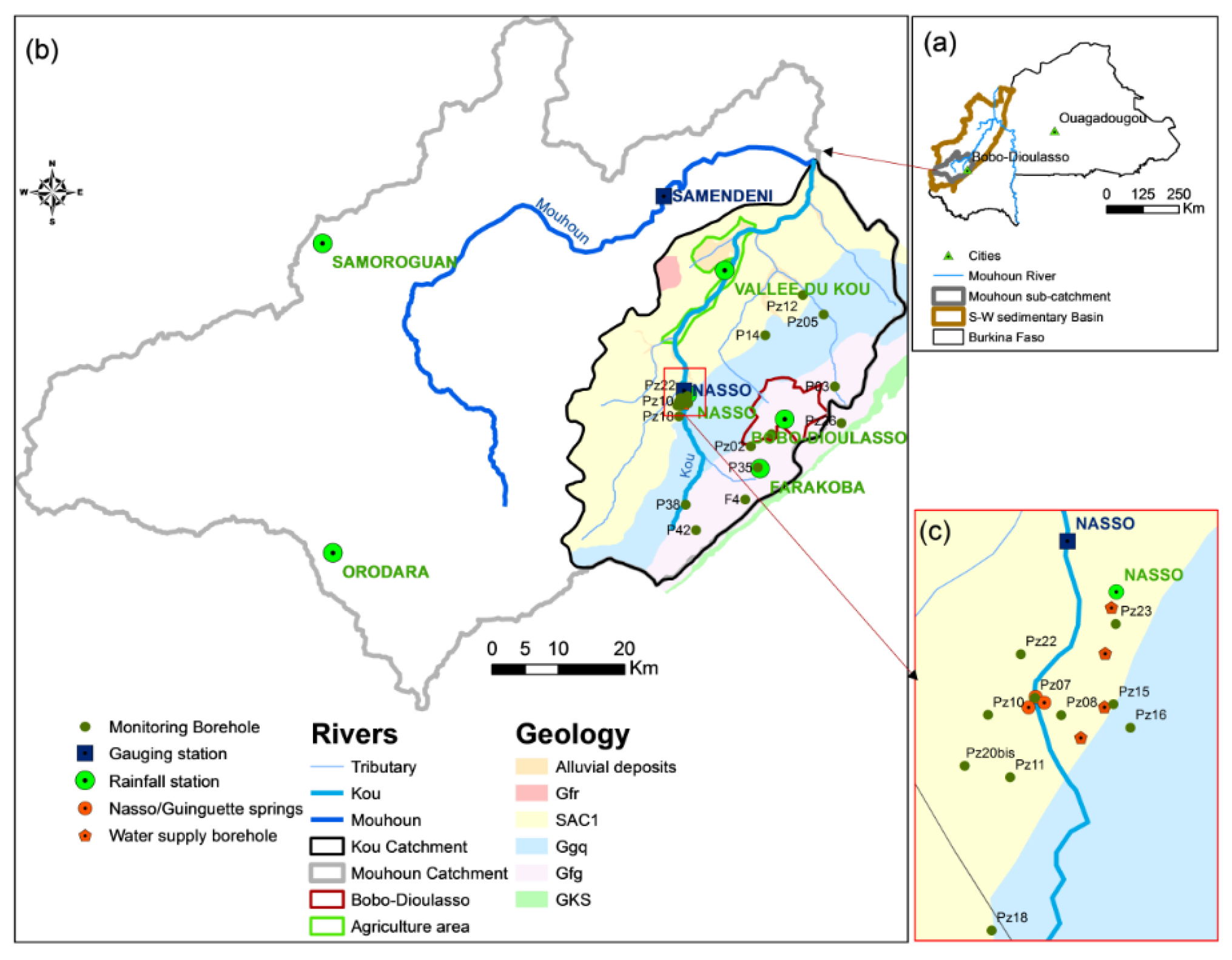
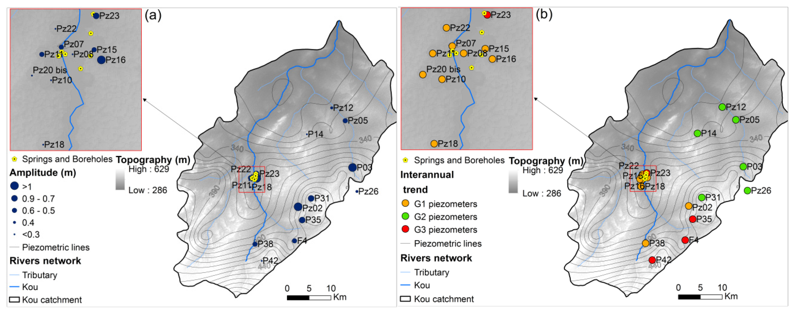
Over the period from 1995 to 2014, the amplitude of seasonal fluctuations ranged from a few centimeters to about 2 m. The highest amplitudes were generally measured in the area close to Bobo-Dioulasso where the altitude is relatively high, and lower amplitudes were measured near the spring area. The variability of the seasonal amplitude reflects the spatial heterogeneity of the groundwater reaction to rainfall (Figure 5a). In the recent period (2007–2014), the amplitudes generally increased compared to the previous period (1995–1999) by a few centimeters to about 70 cm.
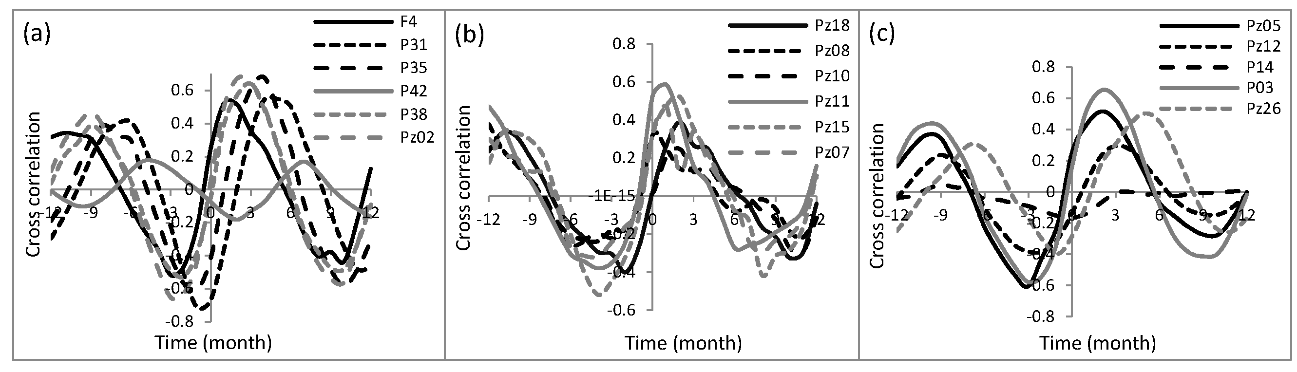
To better characterize the response of the groundwater level, we analyzed the cross-correlation between rainfall and water level in order to estimate the time lag (months) and the magnitude of the correlation. The time lag provides information on the system transfer speed while the magnitude of the correlation indicates the degree of preservation of the rainfall impulse during the transfer [69]. Due to the gaps in the data, this analysis was done on two three-year periods (from 1995 to 1997 and from 2012 to 2014). Figure 6 shows the results for the 1995–1997 period. The rainfall-water level relationship did not change significantly between 1995–1997 and 2012–2014 (not shown), except Pz23, where the maximum correlation decreased from 0.7 to 0.3. Since Pz23 was very close to a pumping zone (about 100 m), this decline could be explained by the disruption of the rainfall signal by pumping.
Most of the piezometers are significantly correlated to rainfall. Typically, the groundwater response to rainfall was delayed by 1–4 months. It reached seven months (with a low correlation) on some piezometers such as P42. The strongest correlations were around 0.6 and lowest around 0.2. Only a few piezometers, including P42 and P14, do not seem to be correlated with rainfall. P42 could be located in a locally-confined area of the aquifer [37]. P14 has the deepest water table (about 85 m), which could explain for the weak correlation between rainfall and water level and the long transfer of the rainfall signal to the groundwater (seven months).

3.4.2. Interannual Variation of Groundwater Level

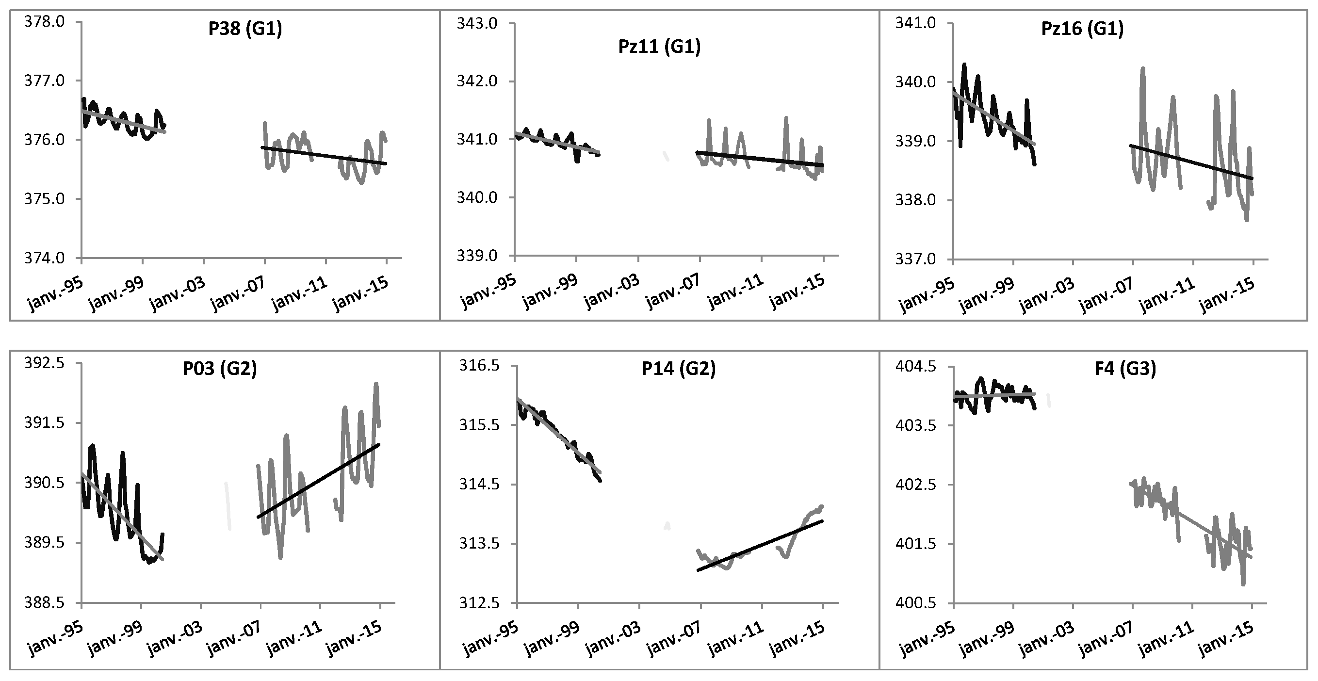
Over the 1995–1999 period, all the piezometers showed a declining groundwater level with a slope ranging from −26 cm/year to −2 cm/year. Only F4 was stable and even showed a slight upward trend of 1 cm/year. After the gap between 2000 and 2006, there is a reduction of the groundwater level slope on all the piezometers. The piezometers were clustered in three groups (G1, G2, and G3) according to their behavior. Figure 4 shows sample piezometers from each group. The water level of the piezometers situated upstream (G1) continued to decline but with a slightly lower slope (Figure 4 and Figure 5b). For piezometers situated downstream of the catchment (G2), the water level rose with a clear slope (5–28 cm/year). Some piezometers (P42, F4, P35, Pz23) had a singular behavior (G3). For instance, F4, which had a stable water level until 1999, then showed a downward trend with a significant slope (−16 cm/year).
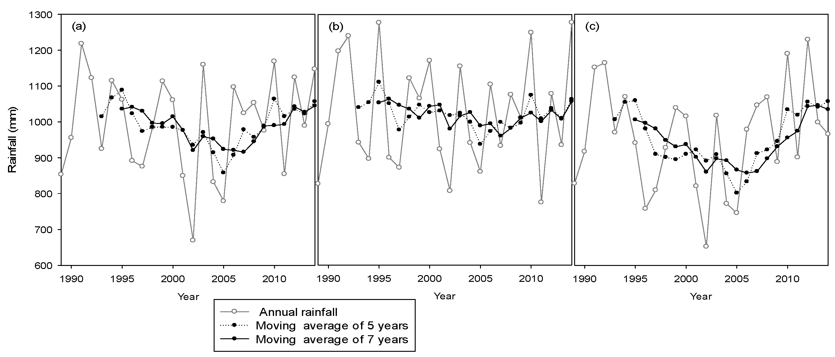
The interannual trend observed on the groundwater level seems to be related to interannual rainfall variability. Over the past 25 years’ rainfall through the five-year and seven-year moving average, displayed a downward trend until 2005, where it began to move upward (Figure 7). This trend reflects observed changes in groundwater levels. However, the exact date of the shift in groundwater levels is not clear because of the data gaps between 2000 and 2006. The similarity between inter-annual groundwater variation and the moving average of rainfall over several years reflects, in some way, a slow and long-term response of the groundwater. The slow response of underground system has been reported by several authors who argue that the rainfall signal is filtered and lagged through the soil and undergound system [5,70]. The aquifer reacts as a low-pass filter that smoothed out the high frequency fluctuations of the rainfall signal [71]. About the slow response of the system, it is also shown that the underground system when subject to a disturbance (changes in boundary conditions) takes some time (few seconds to millions of years), depending on its size and its hydrodynamic characteristics, to recover its equilibrium [72]. This response time can be estimated from the equation of Domenico et al. [73] which applies to a homogeneous, isotropic, and confined aquifer with purely horizontal flow:
τ = L2 × Ss/Kh = L2 × S/T
where τ is the response time [T], L is the length of the aquifer [L], Ss is the specific storage [L−1], Kh is the horizontal hydraulic conductivity [LT−1], S is the storage coefficient [-], and T is the transmissivity [L2T−1].
A transmissivity value of 4 × 10⁻⁴ m2/s, a storage coefficient of 10–4, and a length of 30 km (average size of the catchment) gave a response time on the order of seven years. This is in agreement with the findings from Stoelzle et al. [68] who showed that porous systems such as sandstone have a long-term sensitivity to changes in rainfall and a stronger response to multiyear recharge variability. This slow response of the system was described earlier in Section 3.2 and Section 3.3.
In addition to creating a long term response to climate variability, differences in local hydrodynamic parameters may induce different responses of the groundwater level in space [70,74]. A strong heterogeneity of hydrodynamic parameters due to a difference in the nature of the rock or in the fault lines within the catchment can justify the difference in behavior between upstream and downstream areas. Indeed, a downstream area less transmissive and/or more capacitive than the upstream area can induce this difference.
Other factors such as groundwater withdrawal, land use, vegetation, topography [5,7] may also contributed to a spatial heterogeneity in the response of the groundwater. Given that upstream pumping are not substantially greater (19,800 m3/d out of 40,700 m3/d as a total at the catchment scale) than downstream ones, the assumption of high pumping rates is not a strong argument to justify the difference in behavior between upstream and downstream areas. In connection with topography and land use change, the assumption of higher recharge rates in the downstream area through the surface water, as observed in Southwestern Niger [24] was also put forth but is debatable given that some piezometers are located in a high topography area (P31, Pz26).
The geological and hydrogeological characteristics of the catchment and their spatial variability seem to be the underlying factors of the interannual variation of groundwater level. However, statistical analyses alone cannot be relied on to confirm this hypothesis. Groundwater modeling is required to test it.

3.4.3. Factors Explaining the Spatial and Temporal Variation of the Water Table

The analysis of the piezometric data revealed that the hydrodynamic response of the catchment’s piezometers varies in space (21 piezometers) and time (11 years, 1995–1999, 2007–2009, 2012–2014). We tested the correlations between various environmental factors to explain these differences.
The variables that potentially explain the behavior differences in the 21 piezometers are: the water table depth, the saturated thickness of the aquifer, the altitude of the piezometer reflecting its geomorphological position (plateau, valley), the lithology of the aquifer and the spatiotemporal rainfall variation. The rainfall variable was taken into account using three different variables (annual rainfall, annual effective rainfall, and interannual average rainfall over a number of years).
The groundwater response was characterized by several variables, including:
The interannual variation of groundwater level determined by the difference of the annual average groundwater levels of two consecutive years.
The magnitude of seasonal fluctuations determined by the difference between the highest groundwater level and the lowest groundwater level at the annual scale.
The response time estimated by the rainfall-groundwater level correlation.
The rainfall-groundwater level maximum correlation (Rk) estimated by cross-correlations.
A spatial study was conducted using a PCA based on 21 individuals (the 21 piezometers) and 10 variables or parameters: the four characteristics of the groundwater response above-mentioned, the interannual average rainfall variation and the interannual average effective rainfall variation over the 11 years, the altitude of the piezometer, the lithology of the aquifer, the water table depth, and the saturated thickness of the aquifer. The statistical analyses showed that the geomorphology, the lithology of the aquifer and its saturated thickness are not discriminating parameters of groundwater behavior. The lithology of the aquifer, as described herein, does not reflect well the spatial variability of the transmissivity and the storage coefficient [38]. Specific values of hydrodynamic parameters at each point could have been an explanatory factor of heterogeneous responses as demontred by [70]. Furthermore, the interannual average rainfall variation and the interannual average effective rainfall variation are also nondiscriminating parameters of the groundwater behavior. As described in Section 3.4.2, the response of the groundwater level to the rainfall interannual variability is complex. Rainfall signal is delayed and smoothed through the system so it cannot be correlate directly to groundwater level variation. Thus, these five items were discarded in later analyses.
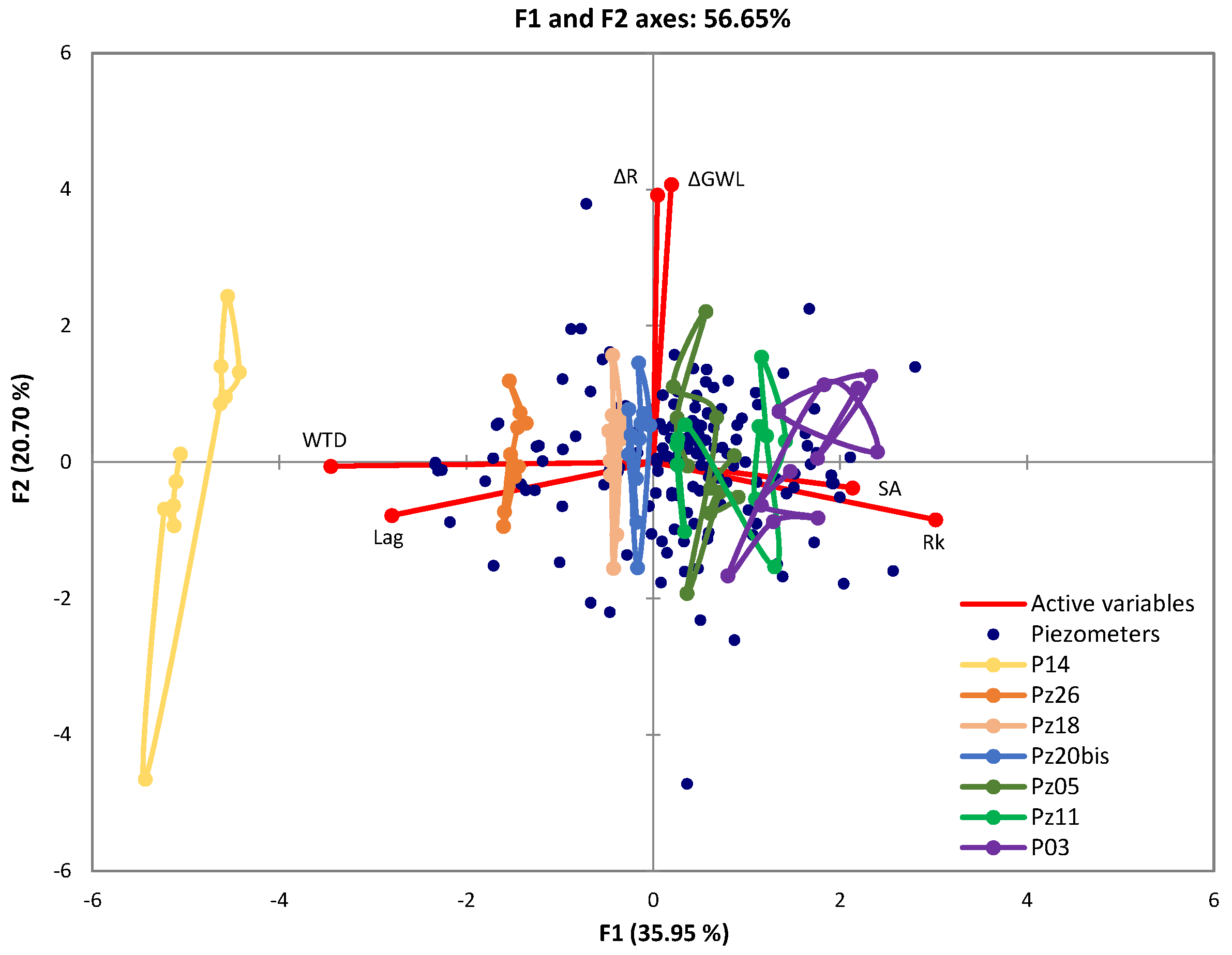
A PCA was performed on 231 individuals (21 piezometers × 11 years) and six variables describing the groundwater behavior and the rainfall forcing (Table 6): groundwater level interannual variations (ΔGWL) and seasonal amplitude (SA) defined for each year, the response time (Lag) and rainfall-groundwater level maximum correlation (Rk) defined for the two periods (1995–1999, 2007–2014), the annual average water table depth (WTD), and the rainfall variation defined by the difference between two consecutive seven-year moving averages (ΔR) calculated for each year. Generally, all these variables displayed different values from one piezometer to another. Only the rainfall value was area-specific, as defined using the Thiessen polygon method.
From the results of the PCA, we retained the first two factorial axes (56% of the variance explained, Table 7) to explain the groundwater spatiotemporal behavior (Figure 8). The first factorial axis (F1) was positively represented by seasonal amplitude and maximal correlation. These two variables contrasted with water table depth and lag. The thicker the unsaturated zone was, the longer the groundwater response time to rainfall was and the less groundwater level was correlated to rainfall. In this case, the groundwater level reacted with a low amplitude. The second axis (F2) was mainly represented by the interannual variation of rainfall and groundwater level. These results were obtained with an average rainfall over several years (seven years), suggesting that the groundwater level interannual variation is the result of the slow response of the groundwater to interannual rainfall fluctuations.
According to these results, rainfall variation explains the temporal variation of the groundwater level on the Y-axis while the spatial variation of the system response is shown on the X-axis. Piezometers are represented globally in two ways. For some of them (e.g., Pz26 or Pz18) with a shallow water table, the individuals are aligned on the Y-axis, showing low sensitivity as regards the spatial response of the underground system (Figure 8). For other piezometers (e.g., P03 or P14), the individuals are dispersed on both the X-axis and the Y-axis, which shows a sensitivity to change in the rainfall and to environmental characteristics (Figure 8). All piezometers were sensitive to changes in rainfall.
The results from the PCA concur with the preceding analyses in Section 3.4.1 and Section 3.4.2. Indeed, the groundwater seasonal variations is strongly linked to the water table depth [69] and explains, to an extent, the spatial variability of the groundwater behavior. Slimani et al. [6] also support that the thicker the surficial formations is, the more the high-frequency variation (inferior to the annual variability) is mitigated in favor of low frequency variation. Considering P14, which has the deepest water level, whilst the groundwater interannual variation is well marked, it has a very low sensitivity to seasonal variations (Figure 4 and Figure 8). Thus, the hydrodynamic characteristics of the aquifers contributed to delay and smooth rainfall signals [70] and, therefore, create a long-term sensitivity to rainfall variability [68].
Factors that govern the groundwater behavior could be further explored if data are available on land use, groundwater abstraction, soils, transmissity, and storage coefficient. At this stage, it can be considered that the results provide some avenues to separate the causes of spatial variability and temporal variability on the groundwater level fluctuation.

4. Conclusions

Time series analysis was used to study both climate variability and its impact on groundwater and to characterize the groundwater response to climate forcings.
This study showed that the Kou catchment underwent the critical episodes of climate variability in West Africa. It has had significant consequences on water resources in general, and on groundwater in particular. Like most catchments in the Sudanian zone, the break observed in the rainfall time series in the 1970s resulted in a larger deficit in flows. This deficit is, nevertheless, on the same order of magnitude as those of heavy rainfall. It also reflects the deficit of the effective rainfall that is also influenced by the increase of evapotranspiration. In the period after 1970, there was no significant change in the Kou catchment’s rainfall time series, suggesting that the drought is actually not yet over, even though rainfall has increased slightly.
The hydrological response of the Mouhoun and Kou catchments to the recent and slight increase in rainfall is influenced by their hydrological precesses. At Nasso, the predominance of water from the deep aquifer, whose response to climate change is slow and smoothed, seems to be the cause of the continuous decrease in flow since 1970. Indeed, although already mostly fed by groundwater before the break, it became almost completely fed by groundwater after the break and the system memory effect became longer. This catchment behavior differs from that of the Mouhoun, a regional system with a high storage capacity whose memory effect has always been long. The catchment functioning of the Mouhoun is strongly related to its base flow, as evidenced by the delay in the resumption of flow compared to the resumption of rainfall in 1990.
The analysis of the piezometric time series, showed that groundwater has a positive response to rainfall with a delay of 1–4 months due to the flow of water through the unsaturated zone. The upward and downward trends observed in groundwater level are the long-term effect of interannual rainfall variations. Indeed, groundwater has a slow response to interannual rainfall variations and this is strongly linked to the physical characteristics of the area (transmissivity, storage coefficient). Given the spatial heterogeneity of these characteristics, the use of tools, such as modeling, is critical to better understand the physical processes that govern the spatiotemporal differences in the groundwater behavior.
The conclusion that one can draw from the foregoing is that the evolution of annual rainfall, alone, is insufficient to understand the impact of climate variability observed on water resources. Changes in heavy rainfall, as well as increased evapotranspiration, are essential to understanding the impact of climate variability on flows and groundwater recharge. The hydrological impact observed is the result of the combined effects of all these changes. The groundwater response to the variability of rainfall largely depends on geological and hydrogeological conditions (water table depth, storage coefficient, and transmissivity) and probably land use. The aquifers’ response to climate variability cannot be studied regardless of the aquifers’ characteristics, which vary in space; hence, the need for modeling. This is the subject of an upcoming article that also includes the effect of water pumping.

Acknowledgments

We wish to extend our thanks to all our donors who provided financial support to this work: Institut de Recherche pour le Développement (IRD) through the Programme Doctoral International “Modélisation des Systèmes Complexes” (PDI/MSC), Office National de l’Eau et de l’Assainissement (ONEA) and UMR Metis (UPMC). We also wish to thank the Direction Générale de la Météorologie (DGM) and the Direction Générale des Ressources en Eau (DGRE) in Burkina Faso for supplying data, PADI/groundwater Project for its support in gathering piezometric data, and the provision of extensive information that greatly enhanced this study. We also thank our two reviewers whose contributions have futher enhanced the quality of this paper.

Author Contributions

The first author conducted this research during her doctoral program under the supervision of Pierre Ribstein, Anne Jost, Angelbert Biaou, and Youssouf Koussoubé. These four authors supervised the data processing, the writing and review of the article. Danièle Valdes-Lao contributed to the statistical analysis and results interpretation.

Conflicts of Interest

The authors declare no conflict of interest.

References

  1. Bates, B.; Kundzewicz, Z.; Wu, S.; Palutikof, J. Climate Change and Water; IPCC Secretariat: Geneva, Switzerland, 2008. [Google Scholar]
  2. Bovolo, C.I.; Parkin, G.; Sophocleous, M. Groundwater resources, climate and vulnerability. Environ. Res. Lett. 2009, 4, 035001. [Google Scholar] [CrossRef]
  3. Hanson, R.T.; Newhouse, M.W.; Dettinger, M.D. A methodology to asess relations between climatic variability and variations in hydrologic time series in the southwestern United States. J. Hydrol. 2004, 287, 252–269. [Google Scholar] [CrossRef]
  4. Hanson, R.T.; Dettinger, M.D.; Newhouse, M.W. Relations between climatic variability and hydrologic time series from four alluvial basins across the southwestern United States. Hydrogeol. J. 2006, 14, 1122–1146. [Google Scholar] [CrossRef]
  5. Gurdak, J.J.; Hanson, R.T.; McMahon, P.B.; Bruce, B.W.; McCray, J.E.; Thyne, G.D.; Reedy, R.C. Climate Variability Controls on Unsaturated Water and Chemical Movement, High Plains Aquifer, USA. Vadose Zone J. 2006, 6, 533–547. [Google Scholar] [CrossRef]
  6. Slimani, S.; Massei, N.; Mesquita, J.; Valdés, D.; Fournier, M.; Laignel, B.; Dupont, J.-P. Combined climatic and geological forcings on the spatio-temporal variability of piezometric levels in the chalk aquifer of Upper Normandy (France) at pluridecennal scale. Hydrogeol. J. 2009, 17, 1823–1832. [Google Scholar] [CrossRef]
  7. Gong, H.; Pan, Y.; Xu, Y. Spatio-temporal variation of groundwater recharge in response to variability in precipitation, land use and soil in Yanqing Basin, Beijing, China. Hydrogeol. J. 2012, 20, 1331–1340. [Google Scholar] [CrossRef]
  8. Hayashi, M.; Farrow, C.R. Watershed-scale response of groundwater recharge to inter-annual and inter-decadal variability in precipitation (Alberta, Canada). Hydrogeol. J. 2014, 22, 1825–1839. [Google Scholar] [CrossRef]
  9. Green, T.R.; Taniguchi, M.; Kooi, H.; Gurdak, J.J.; Allen, D.M.; Hiscock, K.M.; Treidel, H.; Aureli, A. Beneath the surface of global change: Impacts of climate change on groundwater. J. Hydrol. 2011, 405, 532–560. [Google Scholar] [CrossRef]
  10. Scanlon, B.R.; Keese, K.E.; Flint, A.L.; Flint, L.E.; Gaye, C.B.; Edmunds, W.M.; Simmers, I. Global synthesis of groundwater recharge in semiarid and arid regions. Hydrol. Process. 2006, 20, 3335–3370. [Google Scholar] [CrossRef]
  11. Mangin, A. Pour une meilleure connaissance des systèmes hydrologiques à partir des analyses corrélatoire et spectrale. J. Hydrol. 1984, 67, 25–43. [Google Scholar] [CrossRef]
  12. Howard, K.; Griffith, A. Can the impacts of climate change on groundwater resources be studied without the use of transient models? Hydrol. Sci. J. 2009, 54, 754–764. [Google Scholar] [CrossRef]
  13. Taylor, R.G.; Koussis, A.D.; Tindimugaya, C. Groundwater and climate in Africa—A review. Hydrol. Sci. J. 2009, 54, 655–664. [Google Scholar] [CrossRef]
  14. Nicholson, S.E. Climatic variations in the Sahel and other African regions during the past five centuries. J. Arid Environ. 1978, 1, 3–24. [Google Scholar]
  15. Paturel, J.E.; Servat, E.; Delattre, M.O.; Lubes-Niel, H. Analyse de séries pluviométriques de longue durée en Afrique de l’Ouest et Centrale non sahélienne dans un contexte de variabilité climatique. Hydrol. Sci. J. 1998, 43, 937–946. [Google Scholar] [CrossRef]
  16. Le Barbé, L.; Lebel, T.; Tapsoba, D. Rainfall Variability in West Africa during the Years 1950-90. J. Clim. 2002, 15, 187–202. [Google Scholar] [CrossRef]
  17. L’Hôte, Y.; Mahé, G.; Somé, B.; Triboulet, J.P. Analysis of a Sahelian annual rainfall index from 1896 to 2000; The drought continues. Hydrol. Sci. J. 2002, 47, 563–572. [Google Scholar] [CrossRef]
  18. Lebel, T.; Ali, A. Recent trends in the Central and Western Sahel rainfall regime (1990–2007). J. Hydrol. 2009, 375, 52–64. [Google Scholar] [CrossRef]
  19. Panthou, G.; Vischel, T.; Lebel, T. Recent trends in the regime of extreme rainfall in the Central Sahel. Int. J. Climatol. 2014, 34, 3998–4006. [Google Scholar] [CrossRef]
  20. Albergel, J. Sécheresse, désertification et ressources en eau de surface : Application aux petits bassins du Burkina Faso. In the Influence of Climate Change and Climatic Variability on the Hydrologic Regime and Water Resources; IAHS: Oxfordshire, UK, 1987; pp. 355–365. [Google Scholar]
  21. Descroix, L.; Mahé, G.; Lebel, T.; Favreau, G.; Galle, S.; Gautier, E.; Olivry, J.-C.; Albergel, J.; Amogu, O.; Cappelaere, B.; et al. Spatio-temporal variability of hydrological regimes around the boundaries between Sahelian and Sudanian areas of West Africa: A synthesis. J. Hydrol. 2009, 375, 90–102. [Google Scholar] [CrossRef]
  22. Amogu, O.; Descroix, L.; Yéro, K.S.; Le Breton, E.; Mamadou, I.; Ali, A.; Vischel, T.; Bader, J.-C.; Moussa, I.B.; Gautier, E.; et al. Increasing River Flows in the Sahel? Water 2010, 2, 170–199. [Google Scholar] [CrossRef]
  23. Leduc, C.; Favreau, G.; Schroeter, P. Long-term rise in a Sahelian water-table: The Continental Terminal in South-West Niger. J. Hydrol. 2001, 243, 43–54. [Google Scholar] [CrossRef]
  24. Favreau, G.; Cappelaere, B.; Massuel, S.; Leblanc, M.; Boucher, M.; Boulain, N.; Leduc, C. Land clearing, climate variability, and water resources increase in semiarid southwest Niger: A review. Water Resour. Res. 2009, 45. [Google Scholar] [CrossRef]
  25. Descroix, L.; Genthon, P.; Peugeot, C.; Mahé, G.; Abdou, M.M.; Vandervaere, J.-P.; Mamadou, I.; Tanimoun, B.; Amadou, I.; Galle, S.; et al. Paradoxes et contrastes en Afrique de l’Ouest : Impacts climatiques et anthropiques sur les écoulements. Géologues 2015, 187, 47–51. [Google Scholar]
  26. Mahé, G.; Lienou, G.; Bamba, F.; Paturel, J.E.; Adeaga, O.; Descroix, L.; Mariko, A.; Alivy, J.C.; Sangare, S.; Ogilvie, A.; et al. Le fleuve Niger et le changement climatique au cours des 100 dernières années. In Hydro-Climatology: Variability and Change; IAHS: Melbourne, Australia, 2011; pp. 131–137. [Google Scholar]
  27. Mahé, G. Surface/groundwater interactions in the Bani and Nakambe rivers, tributaries of the Niger and Volta basins, West Africa. Hydrol. Sci. J. 2009, 54, 704–712. [Google Scholar] [CrossRef]
  28. Bricquet, J.P.; Bamba, F.; Mahe, G.; Toure, M.; Olivry, J.C. Évolution récente des ressources en eau de l’Afrique atlantique. Revue Sci. L'eau 1997, 10, 321–337. [Google Scholar] [CrossRef]
  29. Mahé, G.; Olivry, J.-C.; Dessouassi, R.; Orange, D.; Bamba, F.; Servat, E. Relations eaux de surface–eaux souterraines d’une rivière tropicale au Mali. Comptes Rendus L'Acad. Sci. Ser. II Earth Planet. Sci. 2000, 330, 689–692. [Google Scholar] [CrossRef]
  30. Kouakou, E.; Koné, B.; N’Go, A.; Cissé, G.; Ifejika Speranza, C.; Savané, I. Ground water sensitivity to climate variability in the white Bandama basin, Ivory Coast. SpringerPlus 2014, 3. [Google Scholar] [CrossRef] [PubMed]
  31. Lutz, A.; Minyila, S.; Saga, B.; Diarra, S.; Apambire, B.; Thomas, J. Fluctuation of Groundwater Levels and Recharge Patterns in Northern Ghana. Climate 2014, 3, 1–15. [Google Scholar] [CrossRef]
  32. Moniod, F.; Pouyaud, B.; Sechet, P. Monographie hydrologique ORSTOM. In le Bassin du Fleuve Volta; ORSTOM: Paris, French, 1977. [Google Scholar]
  33. Ouédraogo, C. Synthèse Géologique de la Région Ouest du Burkina Faso; Programme VREO, SOFRECO-SAWES: Bobo-Dioulasso, Burkina Faso, 2006. [Google Scholar]
  34. Sauret, E.S.G.; Beaujean, J.; Nguyen, F.; Wildemeersch, S.; Brouyere, S. Characterization of superficial deposits using electrical resistivity tomography (ERT) and horizontal-to-vertical spectral ratio (HVSR) geophysical methods: A case study. J. Appl. Geophys. 2015, 121, 140–148. [Google Scholar] [CrossRef]
  35. Sauret, E. Etude des Potentialités Hydrogéologiques d’une Plaine Alluviale en Relation Avec les Eaux Souterraines et de Surface Dans un Contexte D’agriculture Irriguée (Burkina Faso). Ph.D. Thesis, Université de Liège, Liège, Belgium, 2013. [Google Scholar]
  36. Wallens, J.; Compaoré, N.F. Renforcement de la Capacité de Gestion des Ressources en eau dans l’Agriculture Moyennant des Outils de Suivi-Évaluation–GEeau; Rapport Annuel N1 (Décembre 2001–Novembre 2002); Direction Régionale de l’Agriculture, de l’Hydraulique et des Ressources Halieutiques des Hauts Bassins: Bobo Dioulasso, Burkina Faso, 2003. [Google Scholar]
  37. Sogreah Ingenierie. Etude des Ressources en eau Souterraine de la Zone Sédimentaire de la Région de Bobo-Dioulasso; Ministère de l’eau: Bobo-Dioulasso, Burkina Faso, 1994. [Google Scholar]
  38. Gombert, P. Synthèse Sur la Géologie et l’Hydrogéologie de la Série Sédimentaire du Sud-Ouest du Burkina Faso; Programme RESO, IWACO-BURGEAP: Bobo-Dioulasso, Burkina Faso, 1998. [Google Scholar]
  39. Castany, G. Les Eaux Souterraines; Editions Dunod: Paris, French, 1980. [Google Scholar]
  40. Dakouré, D. Etude Hydrogéologique et Géochimique de la Bordure Sud-Est du Bassin Sédimentaire de Taoudéni (Burkina Faso-Mali)-Essai de Modélisation. Ph.D. Thesis, Université Paris VI, Paris, French, 2003. [Google Scholar]
  41. Derouane, J. Modélisation Hydrogéologique du Bassin Sédimentaire; Programme VREO: Bobo-Dioulasso, Burkina Faso, 2008. [Google Scholar]
  42. Sauret, E. Contribution à la Compréhension du Fonctionnement Hydrogéologique du Système Aquifère Dans le Bassin du Kou; Université de Liège: Liège, Belgium, 2008. [Google Scholar]
  43. Huneau, F.; Dakoure, D.; Celle-Jeanton, H.; Vitvar, T.; Ito, M.; Traore, S.; Compaore, N.F.; Jirakova, H.; Le Coustumer, P. Flow pattern and residence time of groundwater within the south-eastern Taoudeni sedimentary basin (Burkina Faso, Mali). J. Hydrol. 2011, 409, 423–439. [Google Scholar] [CrossRef]
  44. Monteith, J. Evaporation and environment. In the State and Movement of Water in Living Organisms; Cambridge University Press: London, UK, 1965; pp. 205–234. [Google Scholar]
  45. Beven, K.J. Rainfall-Runoff Modelling: The Primer; Wiley-Blackwell: Chichester, West Sussex; Hoboken, NJ, USA, 2012. [Google Scholar]
  46. Wheater, H.; Sorooshian, S.; Sharma, K.D. Hydrological modelling in arid and semi-arid areas. In International Hydrology Series; Cambridge University Press: Cambridge; New York, NY, USA, 2008. [Google Scholar]
  47. Thornthwaite, C.W. Thornthwaite An approach toward a rational classification of climate. Geogr. Rev. 1948, 38, 55–94. [Google Scholar] [CrossRef]
  48. Arnold, J.G.; Allen, P.M.; Muttiah, R.; Bernhardt, G. Automated Base Flow Separation and Recession Analysis Techniques. Groundwater 1995, 33, 1010–1018. [Google Scholar] [CrossRef]
  49. Tallaksen, L.M.; Van Lanen, H.A. Hydrological drought: Processes and estimation methods for streamflow and groundwater. In Developments in Water Science; Elsevier: Amsterdam, The Netherlands, 2004. [Google Scholar]
  50. Pettitt, A.N. A Non-Parametric Approach to the Change-Point Problem. Appl. Stat. 1979, 28, 126–135. [Google Scholar] [CrossRef]
  51. Mann, H.B. Nonparametric Tests against Trend. Econometrica 1945, 13, 245–259. [Google Scholar] [CrossRef]
  52. Kendall, M.G. Rank Correlation Method; Griffin: London, UK, 1975. [Google Scholar]
  53. Servat, É.; Paturel, J.E.; Lubès-Niel, H.; Kouamé, B.; Masson, J.M.; Travaglio, M.; Marieu, B. De différents aspects de la variabilité de la pluviométrie en Afrique de l’Ouest et Centrale non sahélienne. Revue Sci. L'eau 1999, 12, 363–387. [Google Scholar] [CrossRef]
  54. Larocque, M.; Mangin, A.; Razack, M.; Banton, O. Contribution of correlation and spectral analyses to the regional study of a large karst aquifer (Charente, France.). J. Hydrol. 1998, 205, 217–231. [Google Scholar] [CrossRef]
  55. Box, G.E.P.; Jenkins, G.; Reinsel, G. Time Series Analysis: Forecasting and Control; Prentice Hall: Englewood Cliffs, NJ, USA, 1994. [Google Scholar]
  56. Lebart, L.; Morineau, A.; Piron, M. Statistique Exploratoire Multidimensionnelle; Dunod: Paris, France, 2002. [Google Scholar]
  57. Mahé, G.; Olivry, J.-C.; Servat, E. Sensibilité des cours d’eau ouest-africains aux changements climatiques et environnementaux: Extrêmes et paradoxes. In Regional Hydrological Impacts of Climatic Change-Hydroclimatic Variability; IAHS: Foz do Iguaçu, Brazil, 2005; pp. 169–177. [Google Scholar]
  58. Orange, D.; Wesselink, A.J.; Mahé, G.; Feitaizoure, C.T. The effects of climate changes on river baseflow and aquifer storage in Central Africa. In Sustainability of Water Resources under Increasing Uncertainty; IAHS: Rabat, Morocco, 1997; pp. 113–123. [Google Scholar]
  59. Descroix, L.; Genthon, P.; Amogu, O.; Rajot, J.-L.; Sighomnou, D.; Vauclin, M. Change in Sahelian Rivers hydrograph: The case of recent red floods of the Niger River in the Niamey region. Glob. Planet. Chang. 2012, 98, 18–30. [Google Scholar] [CrossRef]
  60. Whitley, R.J.; Macinnis-Ng, C.M.O.; Hutley, L.B.; Beringer, J.; Zeppel, M.; Williams, M.; Taylor, D.; Eamus, D. Is productivity of mesic savannas light limited or water limited? Results of a simulation study. Glob. Chang. Biol. 2011, 17, 3130–3149. [Google Scholar] [CrossRef]
  61. Chen, Z.; Grasby, S.E.; Osadetz, K.G. Relation between climate variability and groundwater levels in the upper carbonate aquifer, southern Manitoba, Canada. J. Hydrol. 2004, 290, 43–62. [Google Scholar] [CrossRef]
  62. Ardoin, S.; Lubes-Niel, H.; Servat, E.; Dezetter, A.; Boyer, J.-F.; Mahe, G.; Paturel, J.-E. Analyse de la persistance de la sécheresse en Afrique de l’ouest: caractérisation de la situation de la décennie 1990. In Hydrology of the Mediterranean and Semiarid Regions; IAHS: Montpellier, France, 2003; pp. 355–365. [Google Scholar]
  63. Olivry, J.C.; Bricquet, J.P.; Mahe, G. Vers un appauvrissement durable des ressources en eau de l’Afrique humide? In Hydrology of Warm Humid Regions; IAHS: Wallingford, Oxfordshire, UK, 1993; pp. 67–78. [Google Scholar]
  64. Gárfias-Soliz, J.; Llanos-Acebo, H.; Martel, R. Time series and stochastic analyses to study the hydrodynamic characteristics of karstic aquifers. Hydrol. Process. 2009, 24, 300–316. [Google Scholar] [CrossRef]
  65. Pulido-Bosch, A.; Padilla, A.; Dimitrov, D.; Machkova, M. The discharge variability of some karst springs in Bulgaria studied by time series analysis. Hydrol. Sci. J. 1995, 40, 517–532. [Google Scholar] [CrossRef]
  66. Van Loon, A.F. Hydrological drought explained: Hydrological drought explained. Wiley Interdiscip. Rev. Water 2015, 2, 359–392. [Google Scholar] [CrossRef]
  67. Saft, M.; Peel, M.C.; Western, A.W.; Perraud, J.-M.; Zhang, L. Bias in streamflow projections due to climate-induced shifts in catchment response: Bias in Streamflow Projections. Geophys. Res. Lett. 2016, 43, 1574–1581. [Google Scholar] [CrossRef]
  68. Stoelzle, M.; Stahl, K.; Morhard, A.; Weiler, M. Streamflow sensitivity to drought scenarios in catchments with different geology. Geophys. Res. Lett. 2014, 41, 6174–6183. [Google Scholar] [CrossRef]
  69. Lee, J.-Y.; Lee, K.-K. Use of hydrologic time series data for identification of recharge mechanism in a fractured bedrock aquifer system. J. Hydrol. 2000, 229, 190–201. [Google Scholar] [CrossRef]
  70. Dickinson, J.E.; Hanson, R.T.; Ferré, T.P.A.; Leake, S.A. Inferring time-varying recharge from inverse analysis of long-term water levels. Water Resour. Res. 2004, 40, W07403. [Google Scholar] [CrossRef]
  71. Duvert, C.; Jourde, H.; Raiber, M.; Cox, M.E. Correlation and spectral analyses to assess the response of a shallow aquifer to low and high frequency rainfall fluctuations. J. Hydrol. 2015, 527, 894–907. [Google Scholar] [CrossRef]
  72. Walker, G.R.; Gilfedder, M.; Dawes, W.R.; Rassam, D.W. Predicting Aquifer Response Time for Application in Catchment Modeling. Groundwater 2015, 53, 475–484. [Google Scholar] [CrossRef] [PubMed]
  73. Domenico, P.A.; Schwartz, F.W. Physical and Chemical Hydrogeology; John Wiley: New York, NY, USA, 1998. [Google Scholar]
  74. Bhuiyan, C. Hydrogeological factors: Their association and relationship with seasonal water-table fluctuation in the composite hardrock Aravalli terrain, India. Environ. Earth Sci. 2010, 60, 733–748. [Google Scholar] [CrossRef]
Figure 1. (a) Study area location in Burkina Faso; (b) Mouhoun and Kou catchments with gauging stations, rainfall stations, and monitoring boreholes used in this study; and (c) Nasso-Guinguette springs area.
Water 08 00171 g001
Figure 2. Monthly average rainfall, air temperature, and potential evapotranspiration from 1961 to 2014 at Bobo-Dioulasso station.
Water 08 00171 g002
Figure 3. Autocorrelation of daily flows measured at (a) Samendéni; and (b) Nasso stations for different years; and (c) example of 1966 hydrograph measured at Samendéni; and (d) Nasso stations.
Water 08 00171 g003
Figure 4. Interannual variations of the groundwater levels (m.a.s.l) from 1995 to 2014, for a representative sample of piezometers.
Water 08 00171 g004
Figure 5. Spatial distribution of (a) the amplitude of seasonal fluctuations; and (b) interannual variation according to the clusters G1, G2, and G3 as aforementioned.
Water 08 00171 g005
Figure 6. Cross-correlation between rainfall and groundwater level based on a monthly time step between 1995 and 1997: (a) upstream Kou catchment piezometers; (b) Nasso-Guinguette spring area piezometers; and (c) downstream Kou catchment piezometers.
Water 08 00171 g006
Figure 7. Average annual rainfall and five-year and seven-year moving averages over the past 25 years. (a) Thiessen average rainfall over the Kou catchment; (b) rainfall at the Bobo-Dioulasso station; and (c) rainfall at the vallée du Kou station (most downstream station).
Water 08 00171 g007
Figure 8. PCA of spatial and temporal heterogeneity of the aquifer behavior with a representative sample of piezometers. Analysis with six active variables (Lag, WTD, Rk, SA, ΔR, and ΔGWL).
Water 08 00171 g008
Table 1. Available data used for the present study.
Type of DataStation NameDataPeriodGap Rate (%)Annual Average 1Standard Deviation 1
Climatic dataBobo-DioulassoDaily rainfall1961–20140.21065205
Monthly potential evapotranspiration1961–20140.41958115
Monthly average temperature1961–2014227.20.5
FarakobaMonthly rainfall1953–20145.61048160
NassoMonthly rainfall1953–20124.71042177
Vallée du KouMonthly rainfall1986–20147.5938142
SamoroguanMonthly rainfall1964–20145.41031186
OrodaraMonthly rainfall1954–201411140186
Hydrometric dataSamendéniDaily flow1955–20141814.45.5
NassoDaily flow1961–1997293.71.4
Piezometric data21 piezometersMonthly water level1995–199913–25
2007–201428–39
1 Rainfall unit ”mm” flow unit “m3/s”, evapotranspiration unit “mm”, temperature unit “°C”.
Table 2. Significance level of the Pettitt test.
Corresponding ProbabilityCategory
α < 1%Very significant break
1% < α < 5%Significant break
5% < α < 20%Low significant break
α > 20%Homogeneous series
Table 3. Application of Pettitt tests on Bobo-Dioulasso rainfall indices over 1961–2014. (a) Annual rainfall; and (b) July to September.
Pettitt TestRainfall
Indicesp-value (%)Break DateBreak SignificanceBefore Break 1After Break 1Deficit 2 (%)
(a)P06.41970Low significant118799316
P107.51971Low significant99682417
P3010.71971Low significant49637125
P5012.71970Low significant20911744
(b)P04.31970Significant81463522
P105.71970Low significant71754124
P304.81971Significant38125733
P504.51970Significant19383.857
P0: rainfall > 0 mm, P10: rainfall > 10 mm, P30: rainfall > 30 mm, P50: rainfall > 50 mm; 1 Rainfall unit “mm”; 2 The deficit is the ratio (in %) between the difference of values before and after the break.
Table 4. Results of the break test on Samendéni and Nasso station flows over the period from 1961 to 1997.
StationVariablePettitt TestRainfall and Flow
p-Value (%)Break DateBreak SignificanceBefore Break 1After Break 1Deficit 2 (%)
Bobo-DioulassoRainfall2.111970Significant117798416
SamendéniCatchment rainfall2.551970Significant1177101714
Total flow1.121970Significant19.311.441
Base flow0.471970Very significant14.28.739
Surface flow3.451970Significant5.12.649
NassoCatchment rainfall8.161970Low significant1122100211
Total flow0.01(1970–1974) 3Very significant4.82.743
Base flow0.01(1970–1974) 3Very significant3.72.631
Surface flow0.01(1970–1974) 3Very significant1.10.188
Notes: 1 Rainfall unit “mm” and flow unit “m3/s”.2 Deficit between the 1961–1970 and 1971–1997 periods.3 The date of the break is in this period but is not accurate because of gaps.
Table 5. Results of break test on the Bobo-Dioulasso rainfall station and the Samendéni gauging station from 1971 to 2014, and on the Nasso gauging station1 from 1971 to 1997.
StationVariablePettitt TestRainfall and Flow
p-Value (%)Break DateBreak SignificanceBefore Break 2After Break 2Deficit or Surplus (%) 3
Bobo-DioulassoRainfall43.1No break
SamendéniCatchment rainfall13.81990Low significant99310758
Total flow0.051993Very significant10.215.855
Base flow0.111993Very significant8.112.453
Surface flow0.171990Very significant2.13.463
NassoCatchment rainfall74.1No break
Total flow0.461989Very significant3.012.6313
Base flow0.971983Very significant2.992.5814
Surface flow0.011988Very significant0.220.0959
Notes: 1 The results from Nasso are provided solely for information. Duee to the shortness of the time series (until 1997), the results cannot be deemed to reflect the trend for the recent years.2 Rainfall unit “mm” and flow unit “m3/s”.3 There is a deficit at Nasso and a surplus at Samendéni.
Table 6. Sample data from a piezometer (Pz05) used for the spatiotemporal PCA.
YearΔGWL (m/year)SA (m)Lag (month)RkWTD (m)ΔR (mm/year)
19950.00.642.000.611.50.0
1996−0.20.352.000.611.7−10.0
1997−0.20.732.000.611.8−15.3
1998−0.20.362.000.612.0−32.0
1999−0.10.492.000.612.1−17.9
2007−0.50.472.000.512.6−69.0
20080.00.792.000.512.635.5
20090.20.182.000.512.533.8
20120.10.612.000.512.4112.2
20130.20.222.000.512.22.9
20140.00.402.000.512.2−11.5
Table 7. Principal components from spatio-temporal PCA results.
Factorial axesF1F2F3F4F5F6
Eigenvalues
Eigenvalues2.1571.2421.0290.7650.5400.267
Proportion (%)35.95020.70317.14912.7488.9994.450
Cumulative %35.95056.65473.80386.55195.550100.000
Eigenvectors
WTD−0.597−0.0100.2690.042−0.1150.746
Lag−0.484−0.1350.5380.1040.414−0.525
Rk0.522−0.1460.316−0.0010.6650.404
SA0.369−0.0650.6900.156−0.597−0.056
GWL0.0340.705−0.0040.6980.1210.017
R0.0080.6780.250−0.6890.041−0.030

