Application of Large-Scale, Multi-Resolution Watershed Modeling Framework Using the Hydrologic and Water Quality System (HAWQS)

Abstract

In recent years, large-scale watershed modeling has been implemented broadly in the field of water resources planning and management. Complex hydrological, sediment, and nutrient processes can be simulated by sophisticated watershed simulation models for important issues such as water resources allocation, sediment transport, and pollution control. Among commonly adopted models, the Soil and Water Assessment Tool (SWAT) has been demonstrated to provide superior performance with a large amount of referencing databases. However, it is cumbersome to perform tedious initialization steps such as preparing inputs and developing a model with each changing targeted study area. In this study, the Hydrologic and Water Quality System (HAWQS) is introduced to serve as a national-scale Decision Support System (DSS) to conduct challenging watershed modeling tasks. HAWQS is a web-based DSS developed and maintained by Texas A & M University, and supported by the U.S. Environmental Protection Agency. Three different spatial resolutions of Hydrologic Unit Code (HUC8, HUC10, and HUC12) and three temporal scales (time steps in daily/monthly/annual) are available as alternatives for general users. In addition, users can specify preferred values of model parameters instead of using the pre-defined sets. With the aid of HAWQS, users can generate a preliminarily calibrated SWAT project within a few minutes by only providing the ending HUC number of the targeted watershed and the simulation period. In the case study, HAWQS was implemented on the Illinois River Basin, USA, with graphical demonstrations and associated analytical results. Scientists and/or decision-makers can take advantage of the HAWQS framework while conducting relevant topics or policies in the future.

1. Introduction

In recent years, large-scale watershed modeling has been implemented broadly in the field of water resources planning and management [1,2]. Complex hydrological, sediment, and nutrient processes can be simulated by sophisticated watershed simulation models so that substantial issues such as pollution control, sediment transport, water resources allocation and reservoir operation can be further explored [3,4]. Modelers and decision-makers can take advantage of the scientifically credible results as a reference to conduct corresponding acts or general policies in practice [5].

Several commonly adopted models such as the Agricultural Policy/Environmental eXtender Tool (APEX [6]), Hydrological Simulation Program-Fortran (HSPF [7]), and Soil and Water Assessment Tool (SWAT [8]) are suitable for large-scale analysis. SWAT has been demonstrated to have acceptable performance in terms of model predictions by reflecting anthropogenic activities in detail [9]. SWAT is developed and maintained by the Agricultural Research Service, U.S. Department of Agriculture (USDA-ARS), for the past 30 years. More than 2000 peer-reviewed journal articles are available online for SWAT users as a reference of applications [10]. The operation of SWAT can be fairly straightforward by implementing the user-friendly ArcSWAT interface maintained by Texas A & M University. Similar to the Geographic Information System (GIS), users can delineate the targeted watershed and incorporate essential information such as soil properties, land use type, and conservation practices through step-by-step tutorials. Details of theories and regulated format can be found in the SWAT manual [11].

The calibration/validation of SWAT prior to application is not strictly necessary [11]. However, it is rarely the case that SWAT is deployed without carrying the additional effort of calibration in practice. It is generally performed because better model performance is always more favored in terms of model predictions and referable statistical guidelines [12,13]. In addition, interactions among hydrologic, sediment and nutrient processes may not be reflected accurately by default values of model parameters. To date, model calibration/validation can be conducted by multiple optimization tools such as the Integrated Parameter Estimation and Uncertainty Analysis Tool (IPEAT [14]) and the SWAT Calibration and Uncertainty Procedures (SWAT-CUP [15]). Users are able to perform the calibration/validation process within an affordable timespan depending on the choice of optimization schemes [16].

In considering the efficient tools available to alleviate great effort (specifically the calibration/validation procedure) during watershed modeling, it is still cumbersome to perform tedious initialization steps such as preparing inputs and developing a model with a changing targeted study area. Therefore, a Decision Support System (DSS) that could incorporate input watershed information (e.g., soil data, land use, etc.) with simulation models is required to provide essential assistance [17,18]. In this study, the Hydrologic and Water Quality System (HAWQS [19]) is introduced as a national-scale DSS capable of performing challenging watershed modeling topics. HAWQS is a web-based DSS (designed for the contiguous United States with 48 states) supported by the U.S. Environmental Protection Agency (USEPA) and developed/maintained by Texas A&M University. With the aid of HAWQS, users can generate a SWAT project (default parameters generated by HAWQS have been preliminarily calibrated) within a few minutes by only providing the ending Hydrologic Unit Code (HUC) and the simulation period (note that any watershed project initiated through ArcSWAT may require a further calibration routine to ensure the quality of the simulation performance). The SWAT project provided by HAWQS can be conducted in three different spatial resolutions (HUC8, HUC10, and HUC12) and varying temporal scales (time steps in daily/monthly/annual). In addition, users can specify preferred values of model parameters instead of using the pre-defined sets.

HAWQS has the advanced capacity of integrating watershed modeling in multiple spatial and temporal scales, but there is no research conducted using HAWQS at this time. The major goal of this study is to introduce the framework of HAWQS and the corresponding applications which include the comparisons of performance between HAWQS and ArcSWAT. In the case study, the Illinois River Watershed (IRW) is used to demonstrate the operation of HAWQS in detail. Specifically, the following objectives are defined: (i) to perform a complete setup procedure of HAWQS; (ii) to provide preliminary investigation and comparisons between modeling results of water quantity and quality generated by HAWQS and ArcSWAT; and (iii) to examine watershed output responses using multiple functionalities of HAWQS.

2. Framework of HAWQS and Watershed Modeling

2.1. SWAT Model

The SWAT model is a processed-based, semi-distributed watershed scale simulation model developed by the USDA-ARS [20]. In SWAT, a unique concept of hydrological response units (HRUs) is implemented in which land use, soil type, and land slope are incorporated within each subbasin, respectively. Water balance, sediment and nutrient losses are calculated on the basis of HRUs and summarized for each subbasin for subsequent routing through each reach of the watershed. SWAT has been implemented on various topics such as hydrologic processes, sediment transport, nutrient/carbon discharges, bacteria, and plant growth in the field of water resources, and environmental and agricultural engineering, with a large number of available literature as references [21,22].

SWAT is developed to conduct large-scale watershed simulations with the support of corresponding information [11]. A complete SWAT project can only be formulated through the use of ArcSWAT [23]. However, it can also be potentially challenging to collect and perform the initialization procedure such as collecting field data and delineating the targeted watershed. The development of HAWQS helps to alleviate the time-consuming steps for future users. In addition, user-specified thresholds (e.g., land use, soil types during the grouping step for HRUs) and model parameters can be assigned easily through this tool. Details of HAWQS are introduced in the following sections.

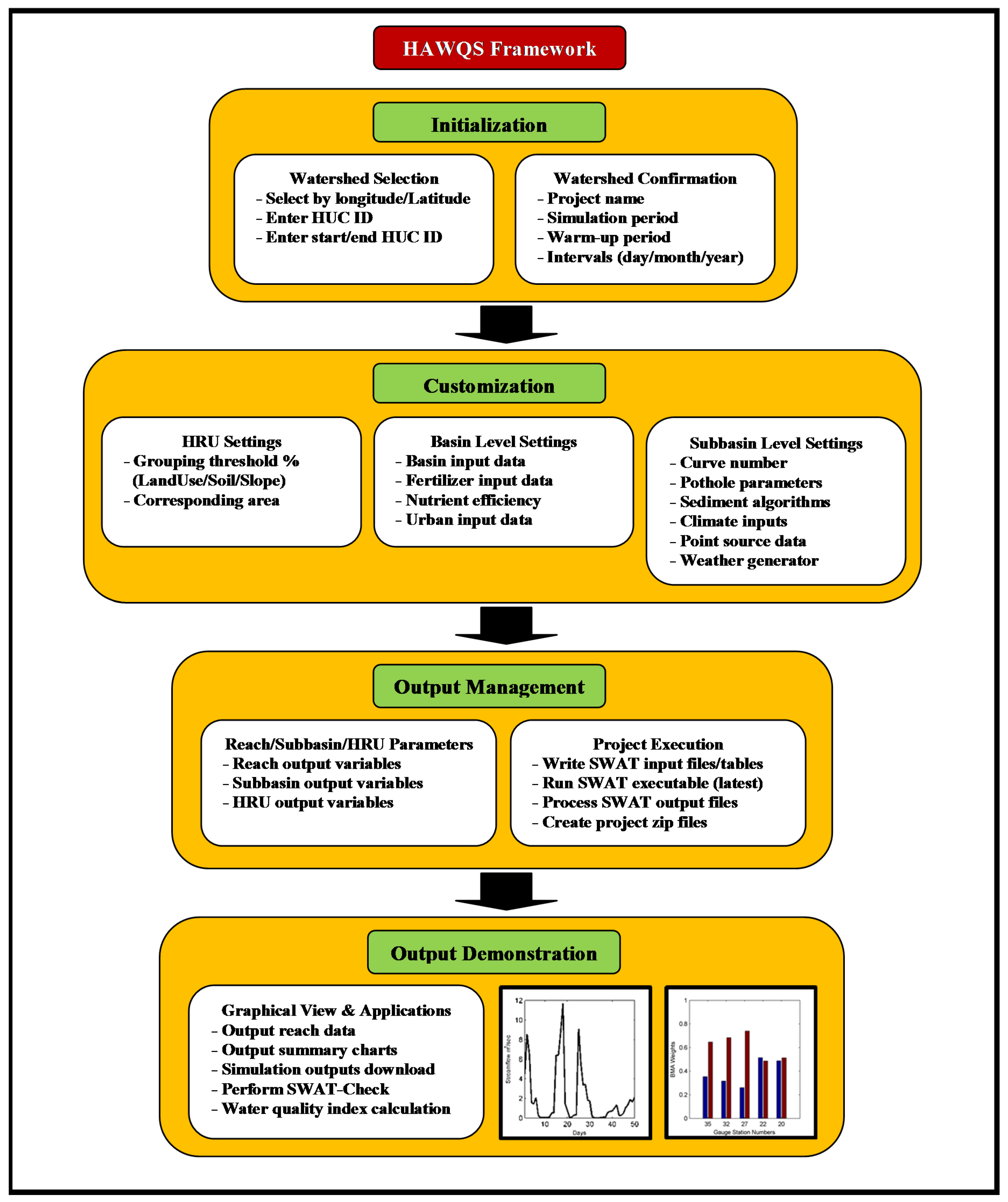
2.2. HAWQS Framework

The operational framework of HAWQS is shown in Figure 1. The HAWQS framework can be grouped into four major categories: (i) initialization; (ii) customization; (iii) output management; and (iv) output demonstration. Since HAWQS is a web-based DSS (servers are located at Texas A&M University), users do not need to have any computational capacity to carry through the process of delineation, simulation, or demonstration. In addition, scheduled computational work (e.g., SWAT simulations) will be continuously carried out even when the web interface is closed. Users have the option to be informed via email when the conducted runs are completed. The data used in HAWQS is briefly described as follows:

• Atmosphere Deposition—National Atmospheric Deposition Program (NADP) [24]
• Climate—Parameter-elevation Regressions on Independent Slopes Model (PRISM) [25]
• Land Use (non-agricultural)—National Land Cover Database (NLCD) [26]
• Land Use (agricultural)—National Agricultural Statistics Service (NASS) [27]
• Reservoirs—National Inventory of Dams (NID) [28]
• River Discharge—United States Geological Survey (USGS) [29]
• Soil—States Derived from the NRCS State Soil Geographic (STATSGO) [30]
• Topography—United States Geological Survey (USGS) [31]
• Water Usage—United States Geological Survey (USGS) [32]

2.2.1. Initialization

There are two major steps of the initialization stage: (i) watershed selection and (ii) watershed confirmation. As shown in Figure 2, three alternatives are available to choose (delineate) the targeted watershed. The first option is designed for beginners who are not familiar with or do not have access to specific HUC ID numbers. In this case, users can enter the projected (or estimated) latitude and longitude to find the proper HUC IDs. In the second option, users can input specific HUC IDs and also check for detail connections as confirmation. If users know the starting and ending HUC IDs exactly, the watershed will be delineated within the range accordingly. In addition, users can select the data resolution during this stage such as HUC8, HUC10, and HUC12.

After the watershed is selected and delineated, users can specify some essential information such as the project name, simulation start/end date, number of warm-up years, printout time steps, and email notifications, which are required for the following simulation process. As shown in Figure 3, the recommended simulation dates are provided in the comments. The total length of the recommended simulation dates is based upon the available weather data such as precipitation and temperature. However, users can still change/add it later if more data is available.

2.2.2. Customization

There are three major steps of the customization stage: (i) HRU settings; (ii) basin level settings; and (ii) subbasin level settings. As shown in Figure 4, users can set the grouping thresholds in percentage for the SWAT project. Land use, soil type, and slope class can be categorized based on minimum percentage values, respectively. In this case, HRUs of three different groups under the specified thresholds will be eliminated. Meanwhile, users can also select any land use that needs to be exempted from the filter.

In SWAT, model parameters can be categorized as basin and subbasin levels. For basin level parameters, the same values will be applied to the entire watershed. On the other hand, subbasin level parameters are more flexible and can be defined for each subbasin or single HRUs. As shown in Figure 4, basin level settings include basin input data, fertilizer input data, nutrient efficiency, urban input data, and land use update. Users can assign preferred values and ranges to basin level parameters for water balance (eight parameters), surface runoff (four parameters), nutrient cycling (seven parameters), and reaches (12 parameters) (see

Table A1. Adjustable SWAT parameters for water balance functions.

Water Balance
Parameter	Description	LB	UB	Default
SFTMP	Snowfall temperature (°C)	−5	5	1
SMTMP	Snow melt base temperature (°C)	−5	5	0.5
SMFMX	Melt factor for snow on 21 June (mm·H2O/°C -day)	0	10	4.5
SMFMN	Melt factor for snow on 21 December (mm·H2O/°C -day)	0	10	4.5
TIMP	Snow pack temperature lag factor	0	1	1
ESCO	Soil evaporation compensation factor	0	1	0.95
EPCO	Plant uptake compensation factor	0	1	1
IPET	Potential evapotranspiration (PET) method [Penman-Monteith/Priestley-Taylor/Hargreaves]

,

Table A2. Adjustable SWAT parameters for surface runoff functions.

Surface Runoff
Parameter	Description	LB	UB	Default
CNCOEF	Plant ET curve number coefficient	0.5	2	1
SURLAG	Surface runoff lag time	0.5	24	4
ICN	Daily curve number calculation method [Soil moisture/Plant Evapotranspiration]
ICRK	Daily curve number calculation method [No model crack flow/Model crack flow in soil]

,

Table A3. Adjustable SWAT parameters for nutrient cycling functions.

Nutrient Cycling
Parameter	Description	LB	UB	Default
RCN	Concentration of nitrogen in rainfall (mg N/L)	0	15	1
CDN	Denitrification exponential rate coefficient	0	3	0
SDNCO	Denitrification threshold water content	0	1	0
NPERCO	Nitrate percolation coefficient	0	1	0.2
PPERCO	Phosphorus percolation coefficient (10 m3/Mg)	10	17.5	10
PHOSKD	Phosphorus soil partitioning coefficient (m3/Mg)	100	200	175
PSP	Phosphorus sorption coefficient	0.01	0.7	0.4

and

Table A4. Adjustable SWAT parameters for functions within reaches.

Reaches
Parameter	Description	LB	UB	Default
MSK_COL1	Calibration coefficient used to control impact of the storage time constant for normal flow	0	10	0
MSK_COL2	Calibration coefficient used to control impact of the storage time constant for low flow	0	10	3.5
MSK_X	Weighting factor controlling relative importance of inflow rate and outflow rate in determining water storage in reach segment	0	0.3	0.2
TRANSRCH	Fraction of transmission losses from main channel that enter deep aquifer	0	1	0
EVRCH	Reach evaporation adjustment factor	0.5	1	0.4
PRF	Peak rate adjustment factor for sediment routing in the main channel	0	2	1
SPCON	Linear parameter for calculating the maximum amount of sediment that can be reentrained during channel sediment routing	0.00001	0.01	0.001
SPEXP	Exponent parameter for calculating sediment reentrained in channel sediment routing	1	1.5	1.2
ADJ_PKR	Peak rate adjustment factor for sediment routing in the subbasin (tributary channels)	0.5	2	0.5
IRTE	Calibration coefficient used to control impact of the storage time constant for normal flow [Variable storage/Muskingum]
IDEG	Channel degradation code [Channel dimension updated No/Yes]
IWQ	In-stream water quality code [In-stream nutrient and pesticide No/Yes]

). For fertilizer input data, 54 combinations of fertilizers are available in the SWAT default. Users can update fertilizer information by changing fractions of mineral N (nitrate and ammonia), mineral phosphorus, organic nitrogen, and organic phosphorus through HAWQS. Users can also adjust the efficiency of fertilizer application in the following table. Similarly, 13 sets of urban input data can also be further tuned by 10 variables such as fraction of total impervious area in urban land type and curb length density in urban land type. Lastly, users have a decision (optional) to update land use data during a simulation run. Details and the corresponding format can be found in the SWAT manual [11].

For subbasin level inputs, users can specify parameter values (e.g., curve number, pothole parameters) or relevant inputs (e.g., sediment routing methods, climate inputs, point sources, and weather generator) in subbasin or HRU levels. For example, the curve number can be adjusted by a percentage increase/decrease to all or selected HRUs. Pothole parameters shown in

Table B1. Adjustable SWAT parameters for pothole functions.

Pothole Parameters
Parameter	Description	LB	UB	Default
POT_FR	Fraction of HRU area that drains into pothole	0	1	0
POT_TILE	Average daily outflow to main channel from tile flow if drainage tiles are installed in the pothole	0	100	0
POT_VOLX	Maximum volume of water stored in the pothole	0	100	0
POT_VOL	Initial volume of water stored in the pothole	0	100	0
SED_CON	Sediment concentration in runoff, after urban BMP is applied	0	5000	0
ORGN_CON	Organic nitrogen concentration in runoff, after urban BMP is applied	0	100	0
ORGP_CON	Organic phosphorus concentration in runoff, after urban BMP is applied	0	50	0
SOLN_CON	Soluble nitrogen concentration in runoff, after urban BMP is applied	0	10	0
SOLP_CON	Soluble phosphorus concentration in runoff, after urban BMP is applied	0	3	0

can be reassigned as preferred values from users. Five alternative sediment routing algorithms are available including the simplified Bagnold’s Equation, Bagnold’s Equation with modifications by each particle size, the Kodoatie model, the Molinas and Wu model, and Yang’s sand and gravel model. Climate inputs and weather generators such as precipitation, temperature, and solar radiation can be further adjusted by percentage for each subbasin and also by specified months. For point source inputs, users can choose to add daily, monthly, yearly, or a constant quantity for pollutants such as nitrate, nitrite, mineral phosphorus and bacteria.

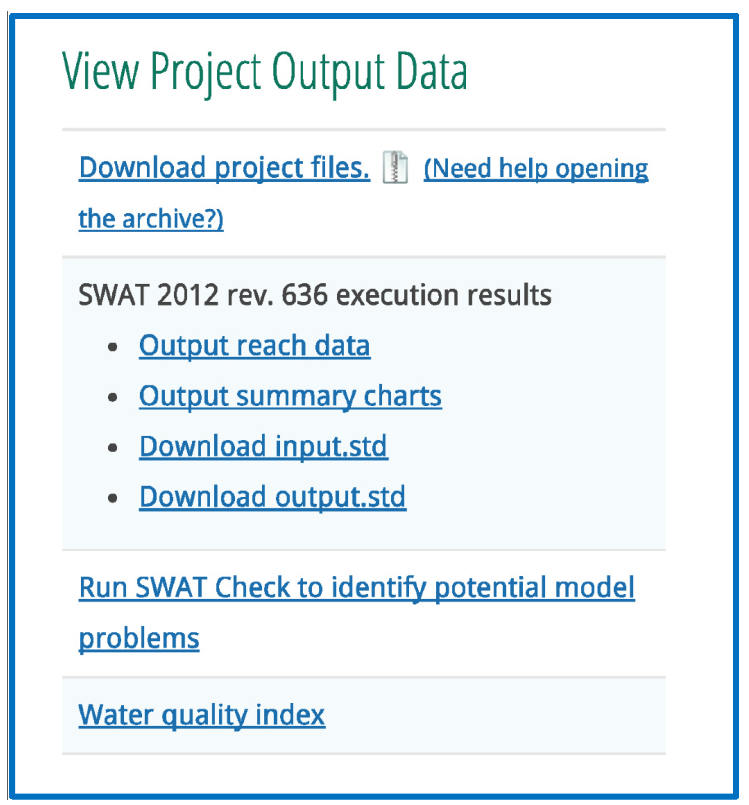
2.2.3. Output Management

In SWAT, simulation outputs can optionally be printed and are saved by changing the settings in the “file.cio” file. HAWQS also provides users with selected outputs to be exported and demonstrated later. As shown in Figure 5, users have optional simulation results for reach output variables (20 in maximum,

Table C1. Printable SWAT variables for reach outputs.

Reach Output Variables
Parameter	Description
FLOW_IN	Average daily streamflow into reach (m3/s)
FLOW_OUT	Average daily streamflow out of reach (m3/s)
EVAP	Average daily loss of water from reach by evaporation (m3/s)
TLOSS	Average daily loss of water from reach by transmission (m3/s)
SED_IN	Sediment transported with water into reach (metric·tons)
SED_OUT	Sediment transported with water out of reach (metric·tons)
SEDCONC	Concentration of sediment in reach (mg/L)
ORGN_IN	Organic nitrogen transported with water into reach (kg·N)
ORGN_OUT	Organic nitrogen transported with water out of reach (kg·N)
ORGP_IN	Organic phosphorus transported with water into reach (kg·P)
ORGP_OUT	Organic phosphorus transported with water out of reach (kg·P)
NO3_IN	Nitrate transported with water into reach (kg·N)
NO3_OUT	Nitrate transported with water out of reach (kg·N)
NH4_IN	Ammonium transported with water into reach (kg·N)
NH4_OUT	Ammonium transported with water out of reach (kg·N)
NO2_IN	Nitrite transported with water into reach (kg·N)
NO2_OUT	Nitrite transported with water out of reach (kg·N)
MINP_IN	Mineral phosphorus transported with water into reach (kg·P)
MINP_OUT	Mineral phosphorus transported with water out of reach (kg·P)
CHLA_IN	Chlorophyll-a transported with water into reach (kg)
CHLA_OUT	Chlorophyll-a transported with water out of reach (kg)
CBOD_IN	Carbonaceous biochemical oxygen demand transported into reach (kg·O2)
CBOD_OUT	Carbonaceous biochemical oxygen demand transported out of reach (kg·O2)
DISOX_IN	Dissolved oxygen transported into reach (kg·O2)
DISOX_OUT	Dissolved oxygen transported out of reach (kg·O2)
SOLPST_IN	Soluble pesticide transported with water into reach (mg a.i.)
SOLPST_OUT	Soluble pesticide transported with water out of reach (mg a.i.)
SORPST_IN	Pesticide sorbed to sediment transported with water into reach (mg a.i.)
SORPST_OUT	Pesticide sorbed to sediment transported with water out of reach (mg a.i.)
REACTPST	Loss of pesticide from water by reaction (mg a.i.)
VOLPST	Loss of pesticide from water by volatilization (mg a.i.)
SETTLPST	Transfer of pesticide from water to river bed sediment by settling (mg a.i.)
RESUSP_PST	Transfer of pesticide from river bed sediment to water by resuspension (mg a.i.)
DIFFUSEPST	Transfer of pesticide from water to river bed sediment by diffusion (mg a.i.)
REACBEDPST	Loss of pesticide from river bed sediment by reaction (mg a.i.)
BURYPST	Loss of pesticide from river bed sediment by burial (mg a.i.)
BED_PST	Pesticide in river bed sediment (mg a.i.)
BACTP_OUT	Number of persistent bacteria transported out of reach (# cfu/100 mL)
BACTLP_OUT	Number of less persistent bacteria transported out of reach (# cfu/100 mL)
CMETAL#1	Conservative metal #1 transported out of reach (kg)
CMETAL#2	Conservative metal #2 transported out of reach (kg)
CMETAL#3	Conservative metal #3 transported out of reach (kg)
TOT_N	Total Nitrogen (kg)
TOT_P	Total Phosphorus (kg)
NO3CONC	Nitrate Concentration (mg/L)

), subbasin output variables (15 in maximum,

Table C2. Printable SWAT variables for subbasin outputs.

Subbasin Output Variables
Parameter	Description
PRECIP	Average total precipitation on subbasin (mm·H2O)
SNOMELT	Snow melt (mm·H2O)
PET	Potential evapotranspiration (mm·H2O)
ET	Actual evapotranspiration (mm·H2O)
SW	Soil water content (mm·H2O)
PERC	Amount of water percolating out of root zone (mm·H2O)
SURQ	Surface runoff (mm·H2O)
GW_Q	Groundwater discharge into reach (mm·H2O)
WYLD	Net water yield to reach (mm·H2O)
SYLD	Sediment yield (metric·tons/ha)
ORGN	Organic N released into reach (kg/ha)
ORGP	Organic P released into reach (kg/ha)
NSURQ	Nitrate released into reach (kg/ha)
SOLP	Soluble P released into reach (kg/ha)
SEDP	Mineral P attached to sediment released into reach (kg/ha)

), and HRU output variables (20 in maximum,

Table C3. Printable SWAT variables for HRU outputs.

HRU Output Variables
Parameter	Description
PRECIP	Total precipitation on HRU (mm·H2O)
SNOFALL	Precipitation falling as snow, sleet, or freezing rain (mm·H2O)
SNOMELT	Amount of snow or ice melting (mm·H2O)
IRR	Amount of irrigation water applied to HRU (mm·H2O)
PET	Potential evapotranspiration (mm·H2O)
ET	Amount of water removed by evapotranspiration (mm·H2O)
SW_INIT	Soil water content at beginning of time period (mm·H2O)
SW_END	Soil water content at end of time period (mm·H2O)
PERC	Amount of water percolating out of the root zone (mm·H2O)
GW_RCHG	Amount of water entering both aquifers (mm·H2O)
DA_RCHG	Amount of water entering deep aquifer from root zone (mm·H2O)
REVAP	Water in shallow aquifer returning to root zone (mm·H2O)
SA_IRR	Amount of water removed from shallow aquifer for irrigation (mm·H2O)
DA_IRR	Amount of water removed from deep aquifer for irrigation (mm·H2O)
SA_ST	Amount of water in shallow aquifer storage at end of time period (mm·H2O)
DA_ST	Amount of water in deep aquifer storage at end of time period (mm·H2O)
SURQ_GEN	Surface runoff generated during time step (mm·H2O)
SURQ_CNT	Surface runoff contribution to reach (mm·H2O)
TLOSS	Amount of water removed from tributary channels by transmission (mm·H2O)
LATQ	Lateral flow contribution to reach (mm·H2O)
GW_Q	Groundwater discharge into reach (mm·H2O)
WYLD	Net amount of water contributed by the HRU to the reach (mm·H2O)
DAILYCN	Average curve number for time period
TMP_AV	Average air temperature for time period (°C)
TMP_MX	Average of daily maximum air temperatures for time period (°C).
TMP_MN	Average of daily minimum air temperatures for time period (°C).
SOL_TMP	Average soil temperature in time period (°C)
SOLAR	Average daily solar radiation for time period (MJ/m2)
SYLD	Amount of sediment contributed by the HRU to the reach (metric·tons/ha)
USLE	USLE soil loss (metric·tons/ha)
N_APP	Amount of N fertilizer applied in regular fertilizer operation (kg·N/ha)
P_APP	Amount of P fertilizer applied in regular fertilizer operation (kg·P/ha)
NAUTO	Amount of N fertilizer applied automatically (kg·N/ha)
PAUTO	Amount of P fertilizer applied automatically (kg·P/ha)
NGRZ	Nitrogen applied to HRU in grazing operation during time step (kg·N/ha)
PGRZ	Phosphorus applied to HRU in grazing operation during time step (kg·P/ha)
CFERTN	Nitrogen applied to HRU in continuous fertilizer operation during time step (kg·N/ha)
CFERTP	Phosphorus applied to HRU in continuous fertilizer operation during time step (kg·P/ha)
NRAIN	Nitrate added in rainfall (kg·N/ha)
NFIX	Amount of N fixed by legumes (kg·N/ha)
F-MN	Transformation of N from fresh organic to mineral pool (kg·N/ha)
A-MN	Transformation of N from active organic to mineral pool (kg·N/ha)
A-SN	Transformation of N from active organic to stable organic pool (kg·N/ha)
F-MP	Transformation of P from fresh organic to mineral (solution) pool (kg·P/ha)
AO-LP	Transformation of P from organic to labile pool (kg·P/ha)
L-AP	Transformation of P from labile to active mineral pool (kg·P/ha)
A-SP	Transformation of P from active mineral to stable mineral pool (kg·P/ha)
DNIT	Amount of N removed from soil by denitrification (kg·N/ha)
NUP	Nitrogen uptake by plants (kg·N/ha)
PUP	Phosphorus uptake by plants (kg·P/ha)
ORGN	Organic N contributed by HRU to reach (kg·N/ha)
ORGP	Organic P contributed by HRU to reach (kg·P/ha)
SEDP	Mineral P attached to sediment contributed by HRU to reach (kg·P/ha)
NSURQ	NO3 contributed by HRU in surface runoff to reach (kg·N/ha)
NLATQ	NO3 contributed by HRU in lateral flow to reach (kg·N/ha)
NO3L	NO3 leached below the soil profile (kg·N/ha)
NO3GW	NO3 contributed by HRU in groundwater flow to reach (kg·N/ha)
SOLP	Soluble phosphorus contributed by HRU in surface runoff to reach (kg·P/ha)
P_GW	Soluble phosphorus contributed by HRU in groundwater flow to reach (kg·P/ha)
W_STRS	Number of water stress days
TMP_STRS	Number of temperature stress days
N_STRS	Number of nitrogen stress days
P_STRS	Number of phosphorus stress days
BIOM	Total plant biomass (metric·tons/ha)
LAI	Leaf area index
YLD	Harvested yield (metric·tons/ha)
BACTP	Persistent bacteria in surface runoff (# cfu/m2)
BACTLP	Number of less persistent bacteria in surface runoff (# cfu/m2)

). In addition, users can select specified HRUs (20 in maximum) for output printing.

To perform model runs, five tasks are available for SWAT simulations (see Figure 5): (i) write SWAT input files; (ii) write SWAT editor tables; (iii) run SWAT 2012 rec. 636 (or the latest SWAT revision); (iv) process SWAT output files; and (v) create downloadable zip of project files. Users can take advantage of these steps as a part of the operating procedure (e.g., manual calibration) by changing parameter values to obtain better-calibrated results. In addition, the conducted SWAT project will be saved as a zip file so that users can use it for the following work with minimum effort.

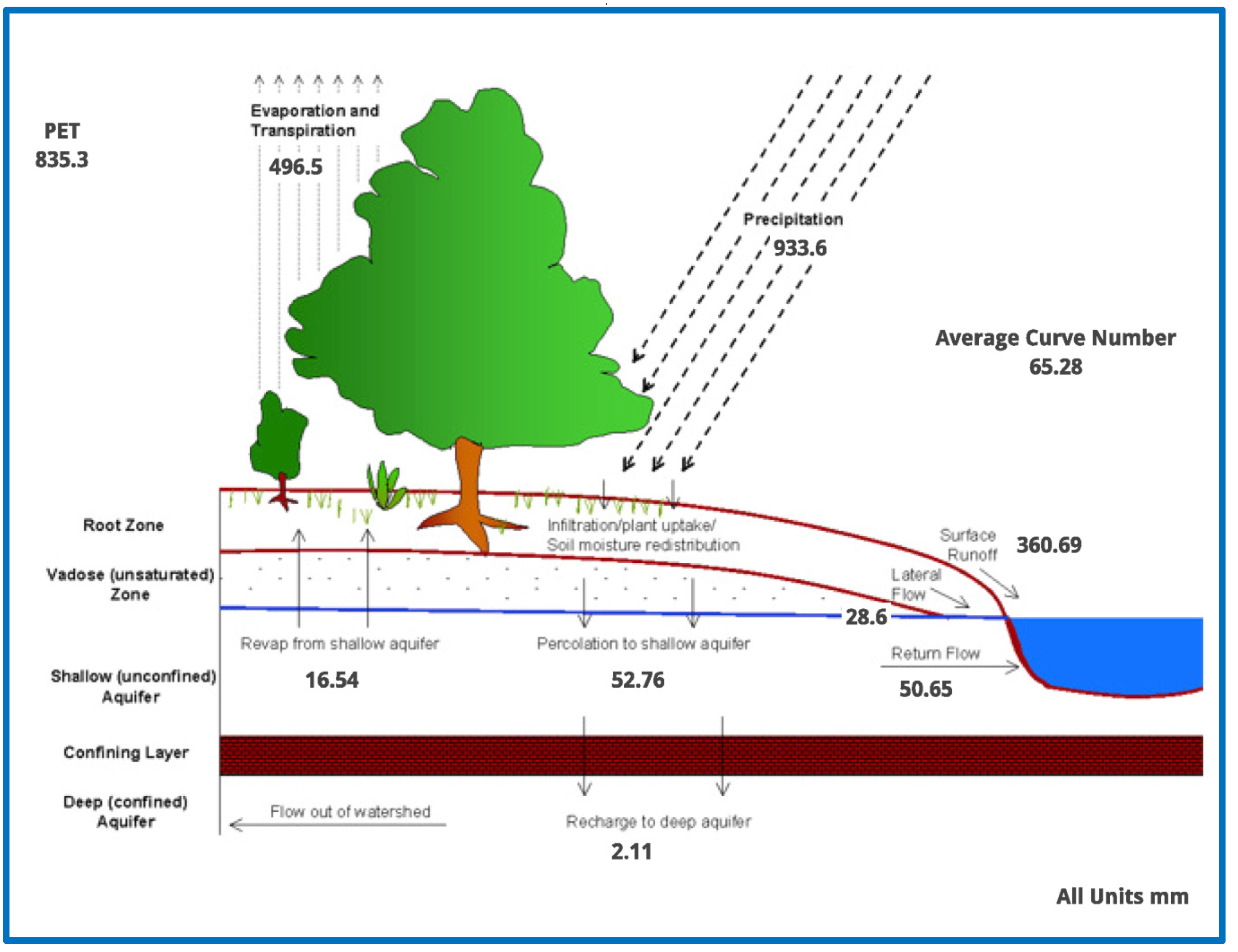
2.2.4. Output Demonstration

After the SWAT project is conducted (see Figure 6), users have options to check error statistics for the corresponding reaches and summary chart for major model responses (e.g., surface runoff, lateral flow, and groundwater). In addition, the post-processing program (SWAT-Check, [33]) and the water quality index [34] are linked with HAWQS to provide professional assessment of model outputs.

SWAT-Check was developed to conduct a stand-alone evaluation of SWAT outputs. A wide variety of model predictions can be demonstrated in graphical fashion so that users can have a better comprehension of the general performance of the model simulation. In HAWQS, it is one of the output options for users to perform SWAT-Check with one click. As shown in Figure 7, hydrological processes such as precipitation, infiltration, and ground water flow can be validated by visually assessable model outputs.

HAWQS provides a Water Quality Index (WQI) which is a composite indicator that combines information from user-defined measurement thresholds from eight water quality parameters into a single overall value (on a 0-to-100 scale). The eight water quality parameters and their measurement thresholds are shown in Figure 8. If no user-defined thresholds are provided, the HAWQS uses the default threshold as recommended by USEPA. The Water Quality Index (0–100) is further used to assign the water bodies as highly impaired (WQI: 0–24.9), boatable (WQI: 25–49.9), fishable (WQI: 50–69.9), swimmable (WQI: 70–94.9), or safe for drinking (WQI: 95+), and associated tabular and spatial information is provided as an output summary. Such information provides guidance for states and tribes to use in adopting water quality standards. It further assists in protecting aquatic life as well as human health.

3. Implementation of the HAWQS

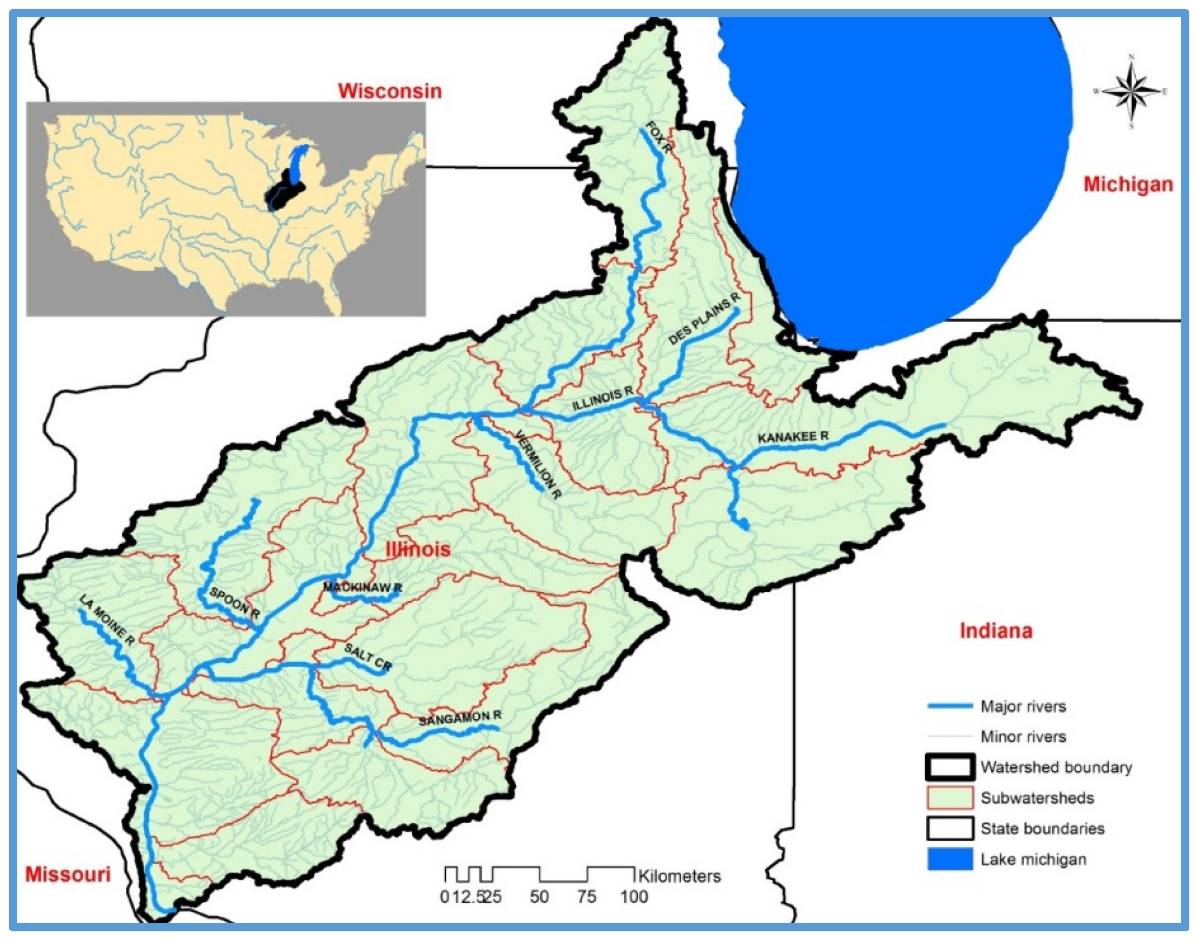
HAWQS was used to conduct watershed simulation on the IRW (Figure 9) at the resolution level of HUC 8. A SWAT project was initiated and evaluated for IRW by the HAWQS web interface. The operational steps and the associated analysis are as follows:

3.1. Study Area

IRW has a drainage area of 74,677 square kilometers and drains 44% of the state of Illinois and about 10,360 square kilometers of area in the states of Indiana and Wisconsin. The Illinois River is approximately 439 km in length and joins the Mississippi River near Grafton, Illinois, approximately 40 km northwest of St. Louis and about 30 km upstream from the confluence of the Missouri and Mississippi rivers. The river is one of the largest tributaries of Mississippi and connects Lake Michigan to the Mississippi River. Major branches and reaches of the IRW include Des Plaines, Kankakee, Iroquois Fox, Vermilion, Mackinaw, Spoon, Sangamon, and La Moine in the states of Illinois, Indiana and Wisconsin. Sedimentation and water quality are major issues in the IRW. As a result, the IRW has become a focus for state and federal agencies and other organizations interested in practices of integrated water management. Several best management practices (BMPs) are being discussed at watershed scale to improve sedimentation, water quality and other relevant issues [35].

3.2. Watershed Setup with the HAWQS Interface

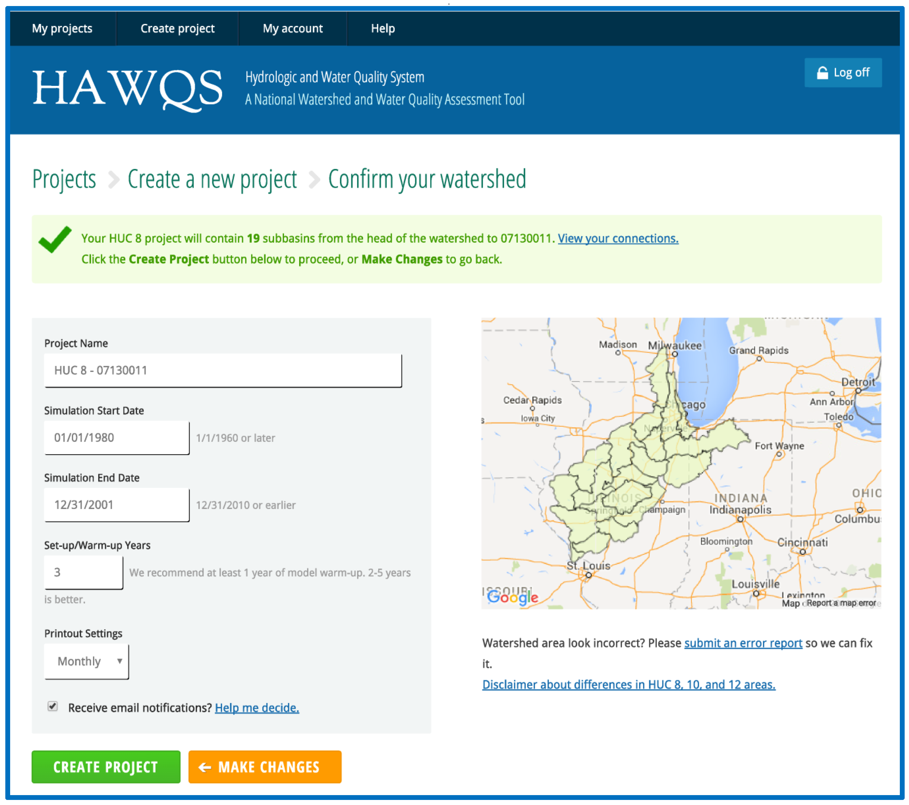
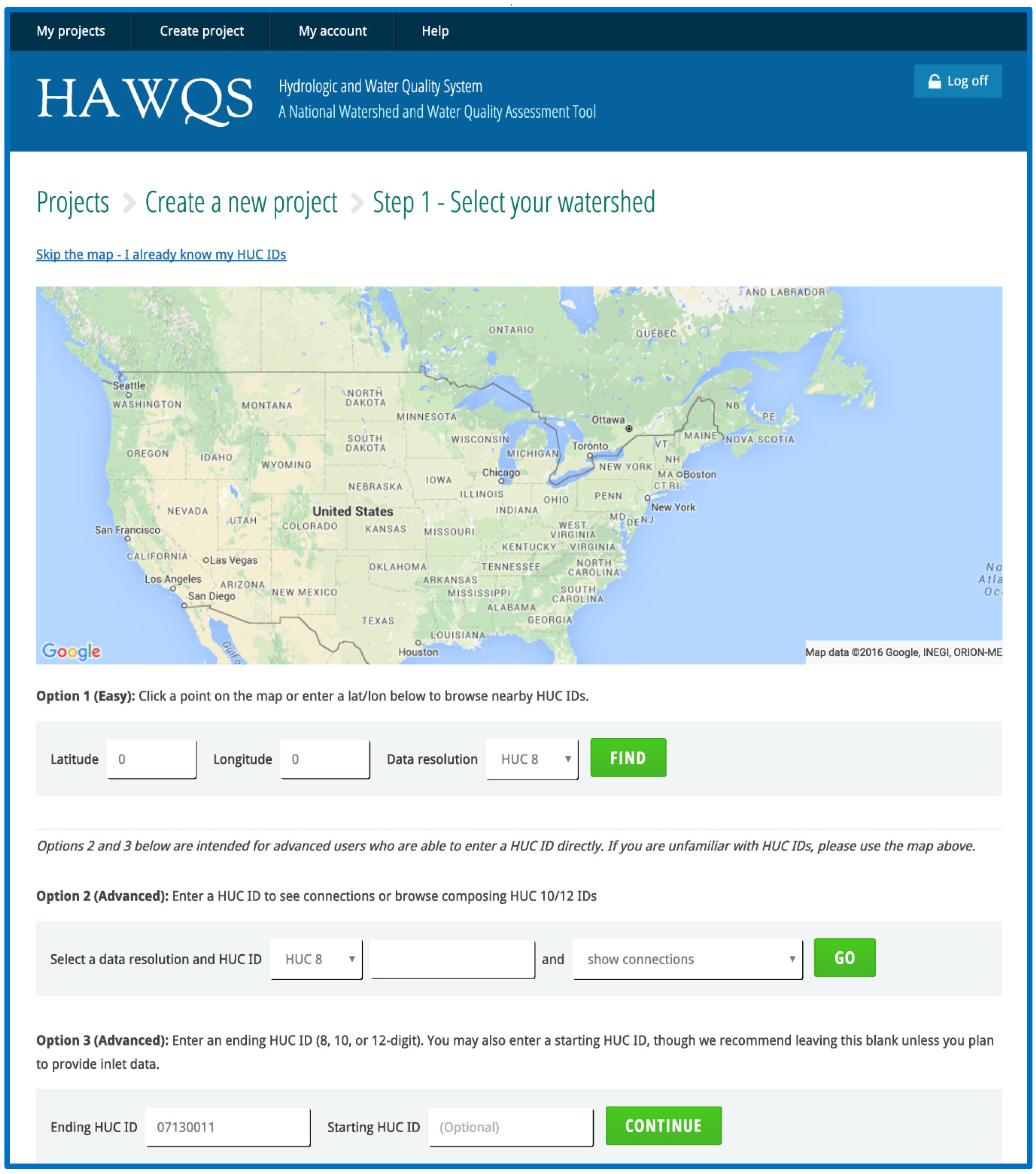
3.2.1. Step 1: Initialization of the Watershed

Upon creating an account, the HAWQS interface gives three options for watershed selection (Figure 2). Option 1 (default option) can be deployed by clicking a point on the map or entering the location of the latitude and longitude. Options 2 and 3 are for advanced users that are able to enter the HUC ID directly. In this study, Option 3 was chosen and the ending HUC 8 ID of 07130011 was entered. This resulted in creating a SWAT model project with 19 subbasins from the head watershed of 07130011 with a start date no earlier than 1960 and an end date no later than 2010.

After the watershed selection is completed, users shall conduct the watershed confirmation (Figure 3). The start and end date of the model simulation was set from the first day of 1980 until the end of 2001 (only for demonstration purposes; different time periods were used in the case study of the later sections) with three years of warm-up period. The printout setting was assigned to be in monthly time steps.

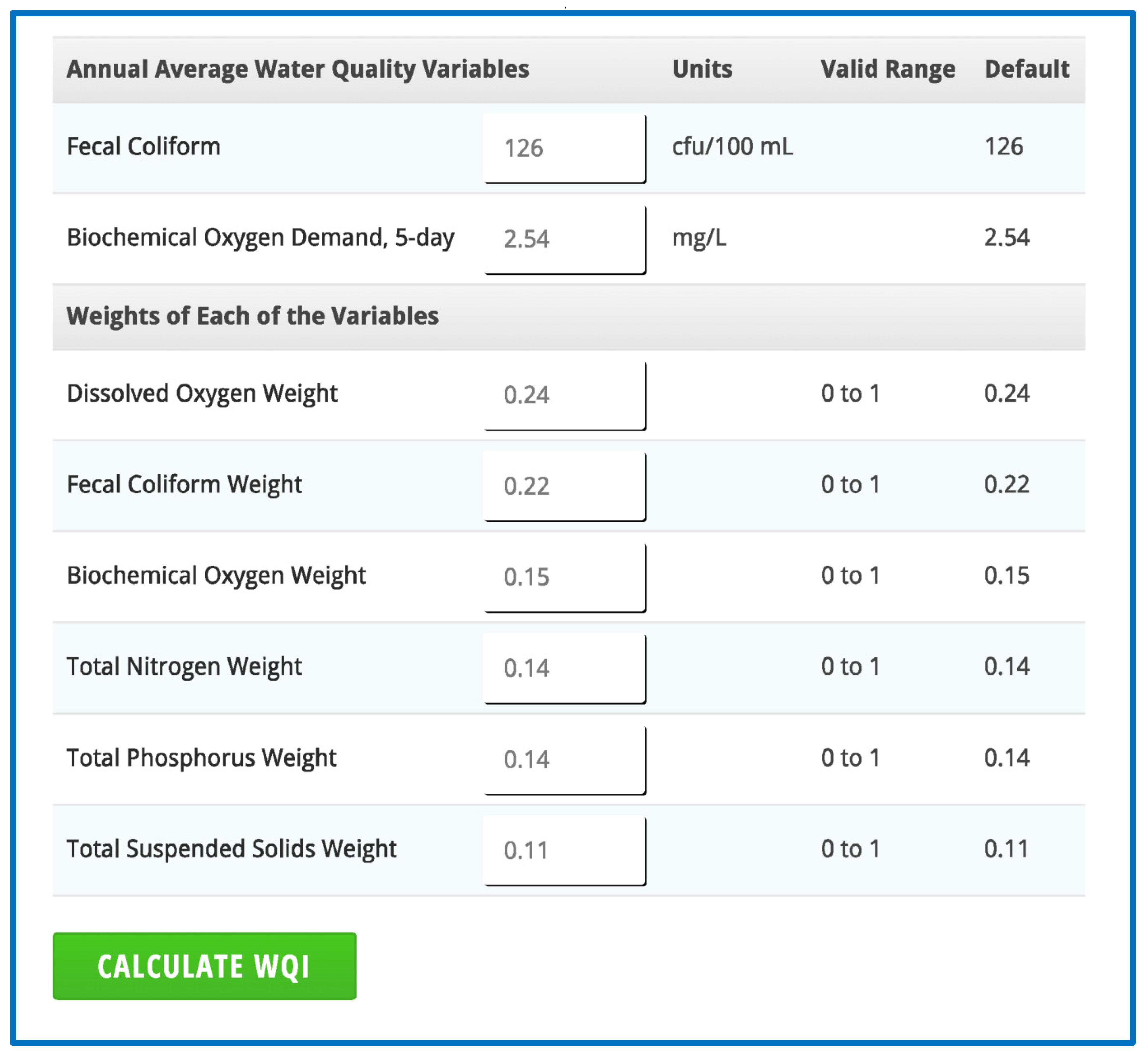
3.2.2. Step 2: Customization of SWAT Input Data

In Step 2, options are available to set HRU thresholds, edit general watershed inputs and databases, edit subbasin inputs, and edit SWAT outputs for printing (Figure 4). In this study, HRU thresholds were set to 4% each for land use, soil and slope categories to eliminate minor land uses, soils, and slopes in each subbasin. This resulted in a significant reduction of HRUs from 4856 to 707. As mentioned previously, users can assign preferred parameter values at HRU, subbasin, and basin levels, respectively. In addition, it was also noted that the HAWQS is capable of providing preliminarily calibrated parameters (as the default) in advance. Therefore, none of the other inputs in terms of the SWAT model parameters were changed in this project.

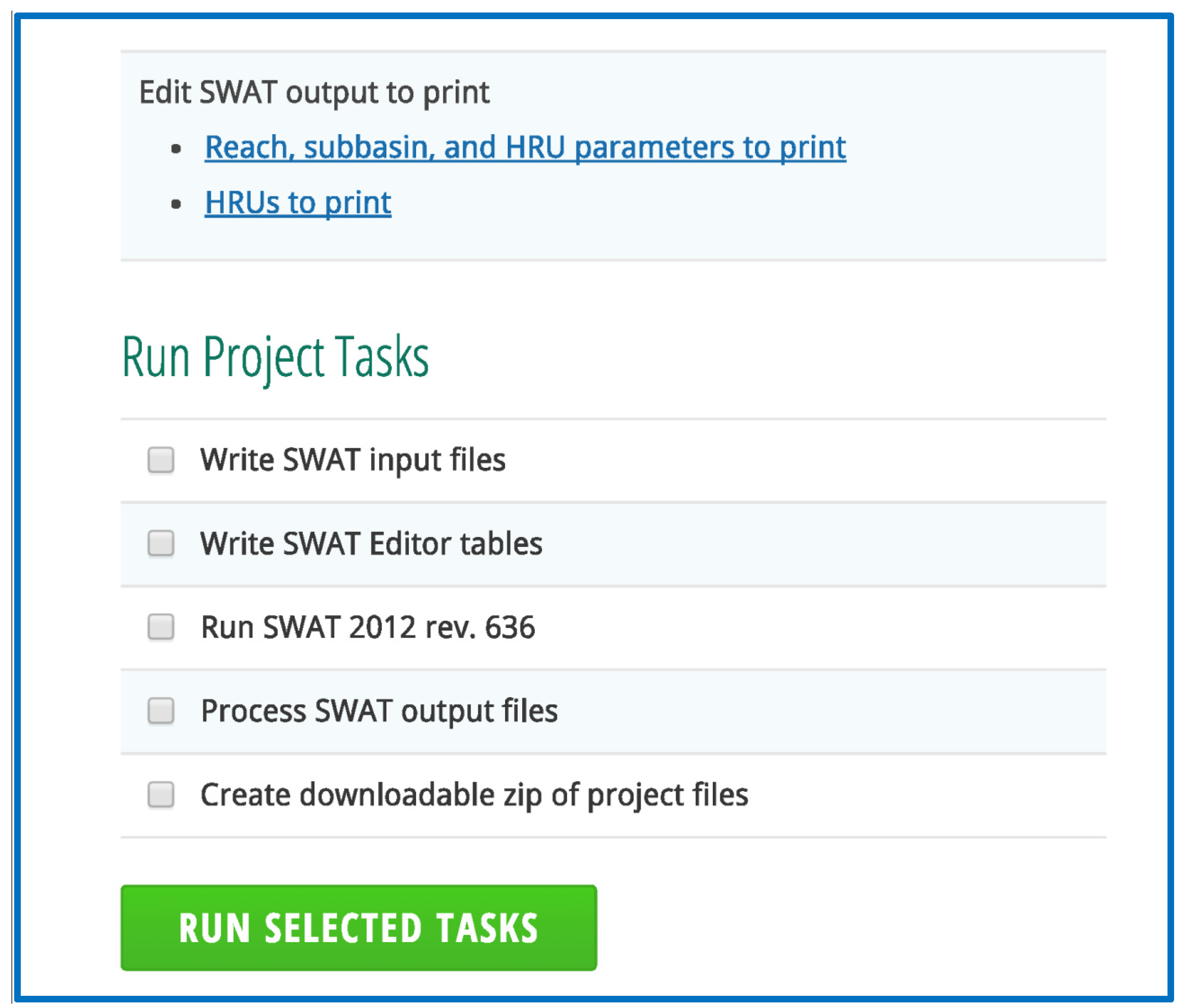
3.2.3. Step 3: Run SWAT Project Tasks

In Step 3, options are available for writing SWAT input files, writing SWAT editor tables, running SWAT 2012 (revision 636), processing SWAT output files, and creating a downloadable zip of project files (Figure 5). In this study, we chose to write SWAT input files, enable SWAT editor tables, run SWAT executable, process SWAT output files, and a create a downloadable zip of project files so that it can be used externally by the SWAT editor program which can read the outputs through the interface. Step 3 is considered not only an easy way of saving/exporting initialized watershed projects, but it also can be used as an online manual calibration framework (manual calibration can be conducted by changing values of specific model parameters through the HAWQS interface) for users to derive results promptly.

3.3. Verification of the SWAT Model

Verification or validation is the process used to demonstrate that the model can produce realistic results in a particular application [36]. The SWAT model was executed for a period of 1980 to 2001 with three years as the warm-up period (1980 to 1982). The results produced by the SWAT model were verified using observed data. Observed data of flow, sediment and nitrogen at the United States Geological Survey (USGS) gauge station (5586100) at Valley City on the Illinois River was used to evaluate the model performance. Verification was done in two time periods to make sure the model simulations are temporally reasonable. In the case study, the first time period selected was from 1983 to 1989 and the second period was 1990 to 2001.

3.4. Results

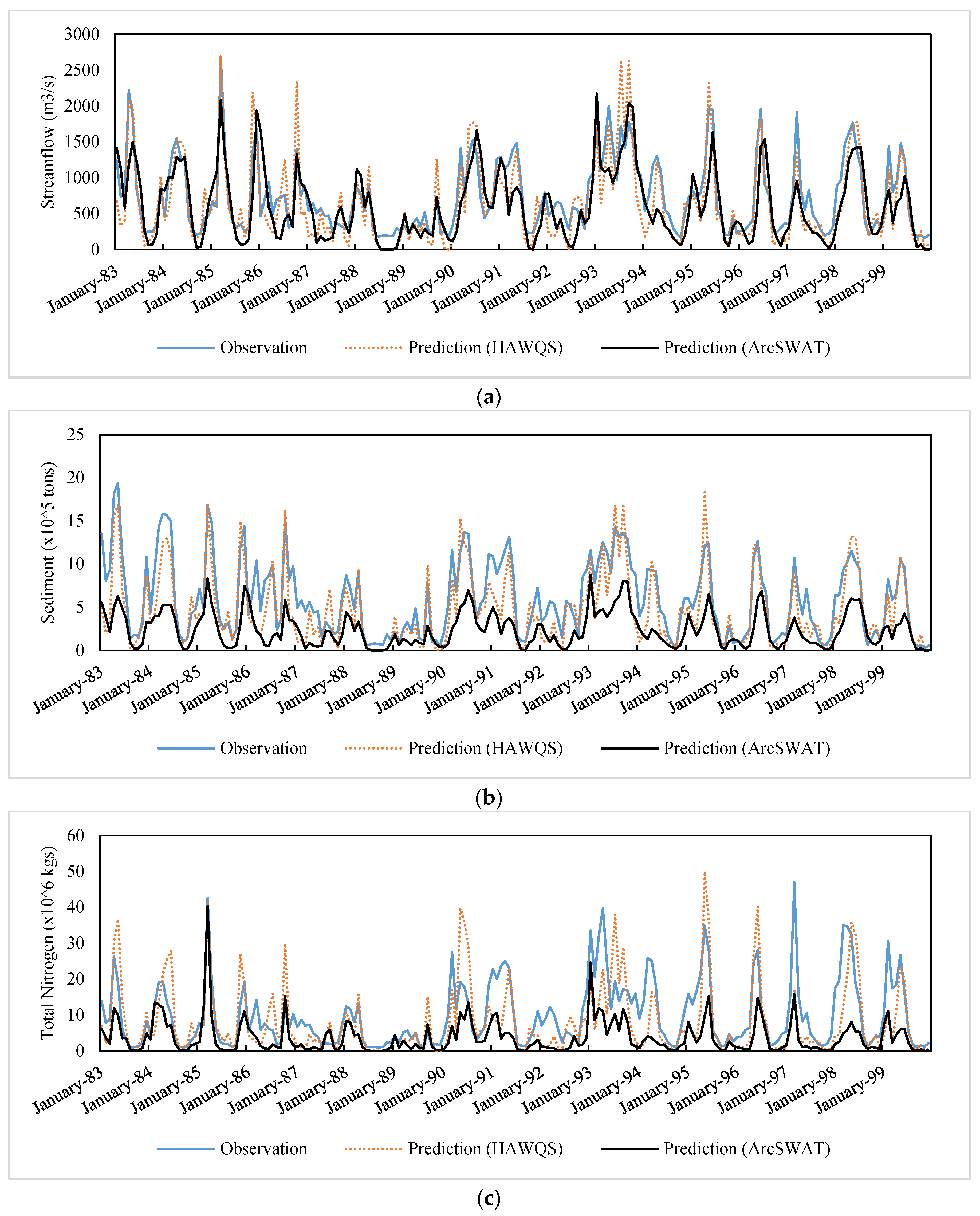
3.4.1. Results of Calibration and Validation

In order to demonstrate the improvement in terms of model performance between HAWQS and ArcSWAT, another IRW project was conducted by ArcSWAT.

Table 1. Error statistics for monthly flow, sediment and total nitrogen (TN) for calibration (1983–1989) and validation (1990–2001) periods.

Output Variables	IRW (HAWQS)				IRW (ArcSWAT)
	Calibration		Validation		Calibration		Validation
	NSE	PBIAS (%)	NSE	PBIAS (%)	NSE	PBIAS (%)	NSE	PBIAS (%)
Flow	0.70	8.51	0.72	13.91	0.61	7.86	0.49	21.1
Sediment	0.66	26.55	0.67	19.07	−0.05	61.56	−0.14	57.86
Total Nitrogen	0.36	−4.15	0.23	26.78	0.26	45.14	−0.22	68.54

NSE: Nash Sutcliffe Efficiency coefficient; PBIAS: Percent bias; IRW: Illinois River Basin.

shows summary statistics of the Nash-Sutcliffe Efficiency coefficient (NSE (Equation (1) [13,37]) and Percent Bias (PBIAS (Equation (2) [12,13]) for monthly flow, sediment and total nitrogen (TN) for calibration and validation time periods. In both questions, $y_i^{Obs}$ is the observed data at time step $i$; $y_i^{Sim}$ is the simulated model output at time step $i$; $y_i^{Mean}$ is the average observed data at time step $i$; $N$ is the total time span. As shown in

Table 2. Quantitative criteria categorized by the General Performance Ratings [12].

Performance Rating	NSE	PBIAS (%)
		Streamflow	Sediment	Nitrogen
Very Good	0.75 < NSE ≤ 1.00	PBIAS < ±10	PBIAS < ±15	PBIAS < ±25
Good	0.65 < NSE ≤ 0.75	±10 ≤ PBIAS < ±15	±15 ≤ PBIAS < ±30	±25 ≤ PBIAS < ±40
Satisfactory	0.50 < NSE ≤ 0.65	±15 ≤ PBIAS < ±25	±30 ≤ PBIAS < ±55	±40 ≤ PBIAS < ±70
Unsatisfactory	NSE ≤ 0.50	PBIAS ≥ ±25	PBIAS ≥ ±55	PBIAS ≥ ±70

NSE: Nash-Sutcliffe efficiency coefficient; PBIAS: Percent bias.

, the General Performance Ratings (GPR) were implemented as the quantitative criteria recommended by Moriasi et al. [12] and the monthly time step was used to evaluate the model performance.

$$NSE=1-\frac{{\sum }_{i=1}^N{\left(y_i^{Obs}-y_i^{Sim}\right)}^2}{{\sum }_{i=1}^N{\left(y_i^{Obs}-y_i^{Mean}\right)}^2}$$

(1)

$$PBIAS=\frac{100{\sum }_{i=1}^N{\left(y_i^{Obs}-y_i^{Sim}\right)}^{}}{{\sum }_{i=1}^N{\left(y_i^{Obs}\right)}^{}}$$

(2)

In the first time period (1983–1989), the model performance by HAWQS was considered good for flow and sediment and unsatisfactory for TN as per NSE criteria. As per PBIAS criteria, the model performance was considered “Very Good” (also see Table 1) for flow and TN and good for sediment. In the second time period (1990–2001) period, the model performance was considered good for flow, sediment and unsatisfactory for TN as per NSE criteria. The model performance was good for flow, sediment and TN based on PBIAS criteria. On the other hand, results generated by ArcSWAT are considerably worse than HAWQS. Flow simulation (“Satisfactory”) in the calibration period is the only output variable that had a performance better than unsatisfactory. Predictions for sediment and total nitrogen are evidently far away from acceptable (NSE values are mostly negative with fairly high PBIAS compared to the results from HAWQS).

The time series comparisons between observed and predicted flow, sediment and TN for the calibration and validation periods are shown in Figure 10. Comparisons of temporal processes show that the model predictions of HAWQS were in close agreement with the observed data. In addition, it is clear that temporal processes generated by ArcSWAT are apparently off the major trend and typically underestimated. It was mentioned previously that further calibration using auto-calibration tools (e.g., IPEAT, SWAT-CUP) after downloading the SWAT model from the HAWQS interface (or ArcSWAT) will improve the statistics as well as agreements of temporal time series. However, one of the major advantages of HAWQS is identifying the targeted area and providing supplementary information (e.g., model predictions of flow, sediment, and total nitrogen) within fairly short periods of time which cannot be done by ArcSWAT. The availability of general functions between HAWQS and ArcSWAT are compared in

Table 3. General comparisons between HAWQS and ArcSWAT.

Comparisons	HAWQS	ArcSWAT
Graphical Demonstration	Available	Not Available
Available to assign preferred parameter values	Available	Not Available
Available for remote simulation	Available	Not Available
Data Collection	No Need	Required
Calibration requirement	No Need	Required
Required Software	No Need	ArcSWAT
Required Hardware	Regular Desktop	Regular Desktop
Spatial resolution	3 Options	Not Available
Operation time	Few Minutes	Hours at Minimum

. Demonstrated limitations of ArcSWAT indicated that the dominant improvements by HAWQS over ArcSWAT have shown great advantages not only in timely matters (e.g., urgent requests need immediate solutions) but also in general applications.

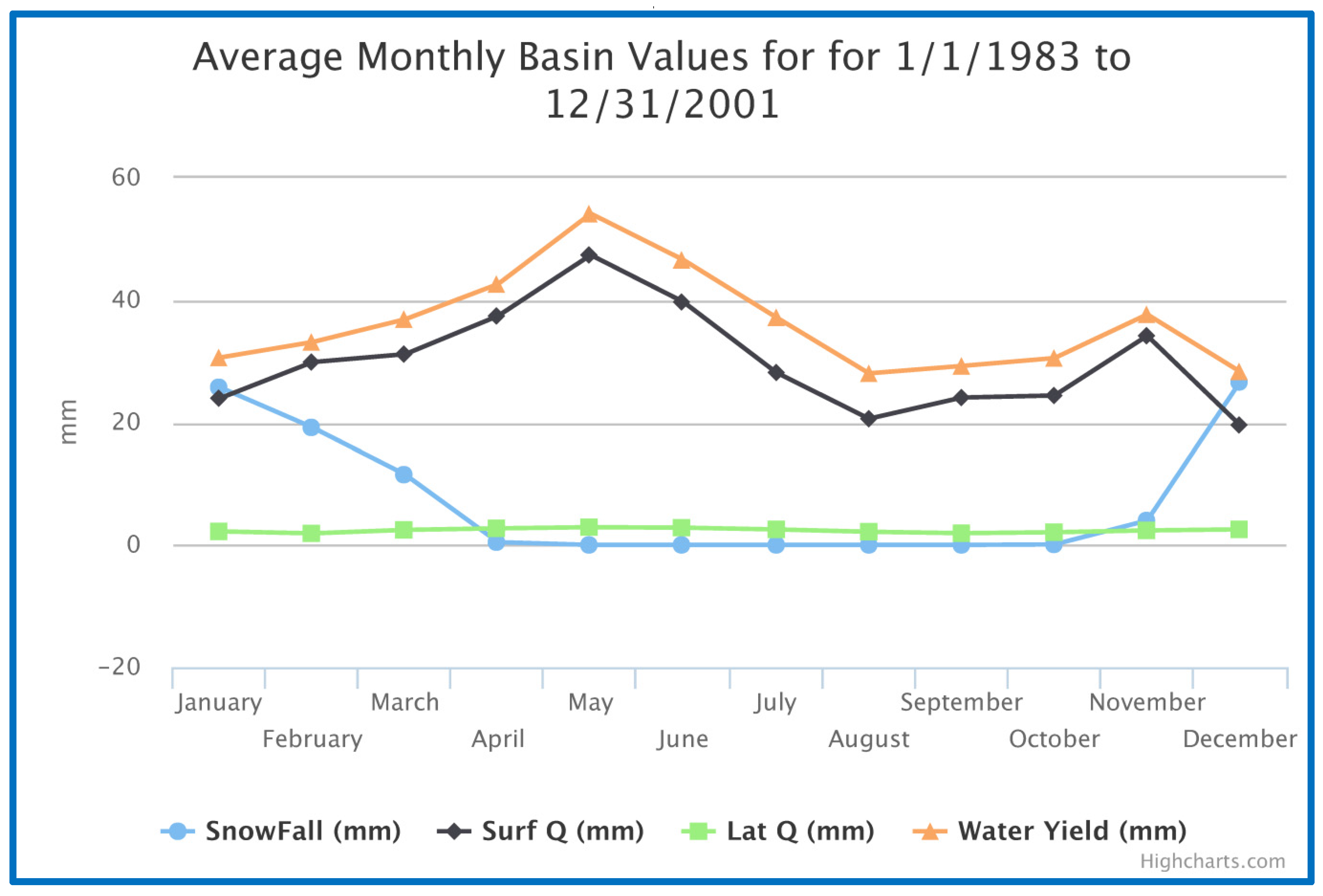
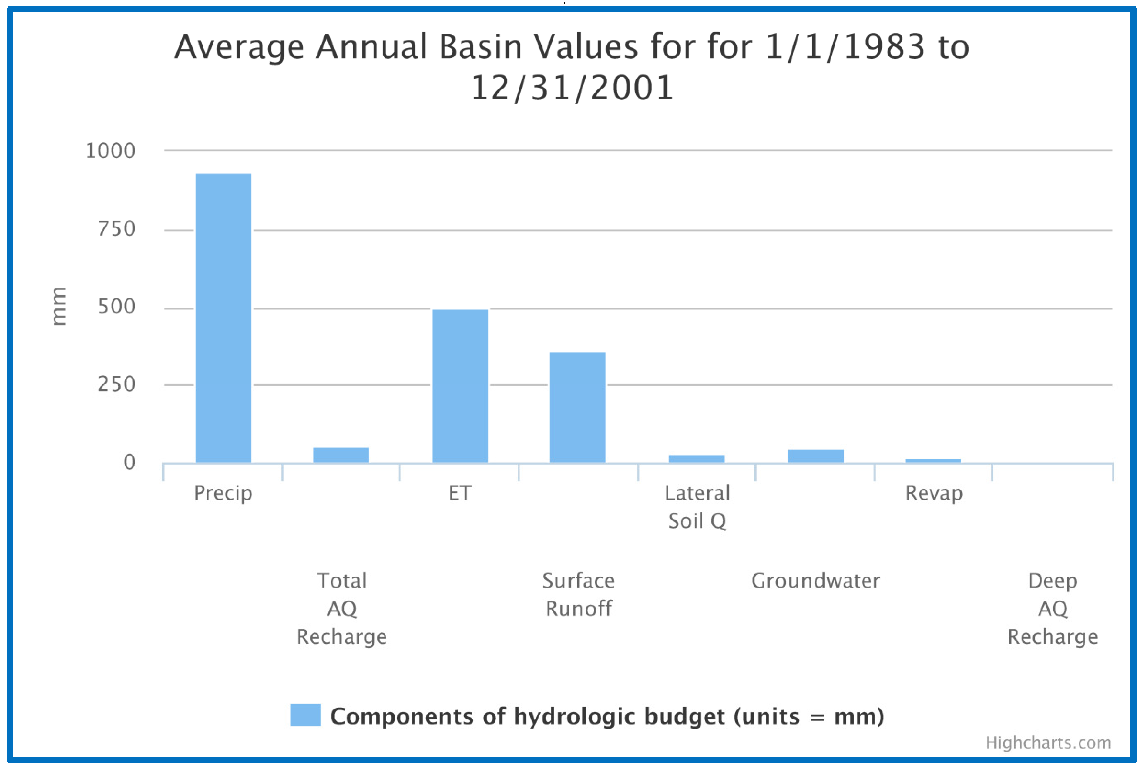
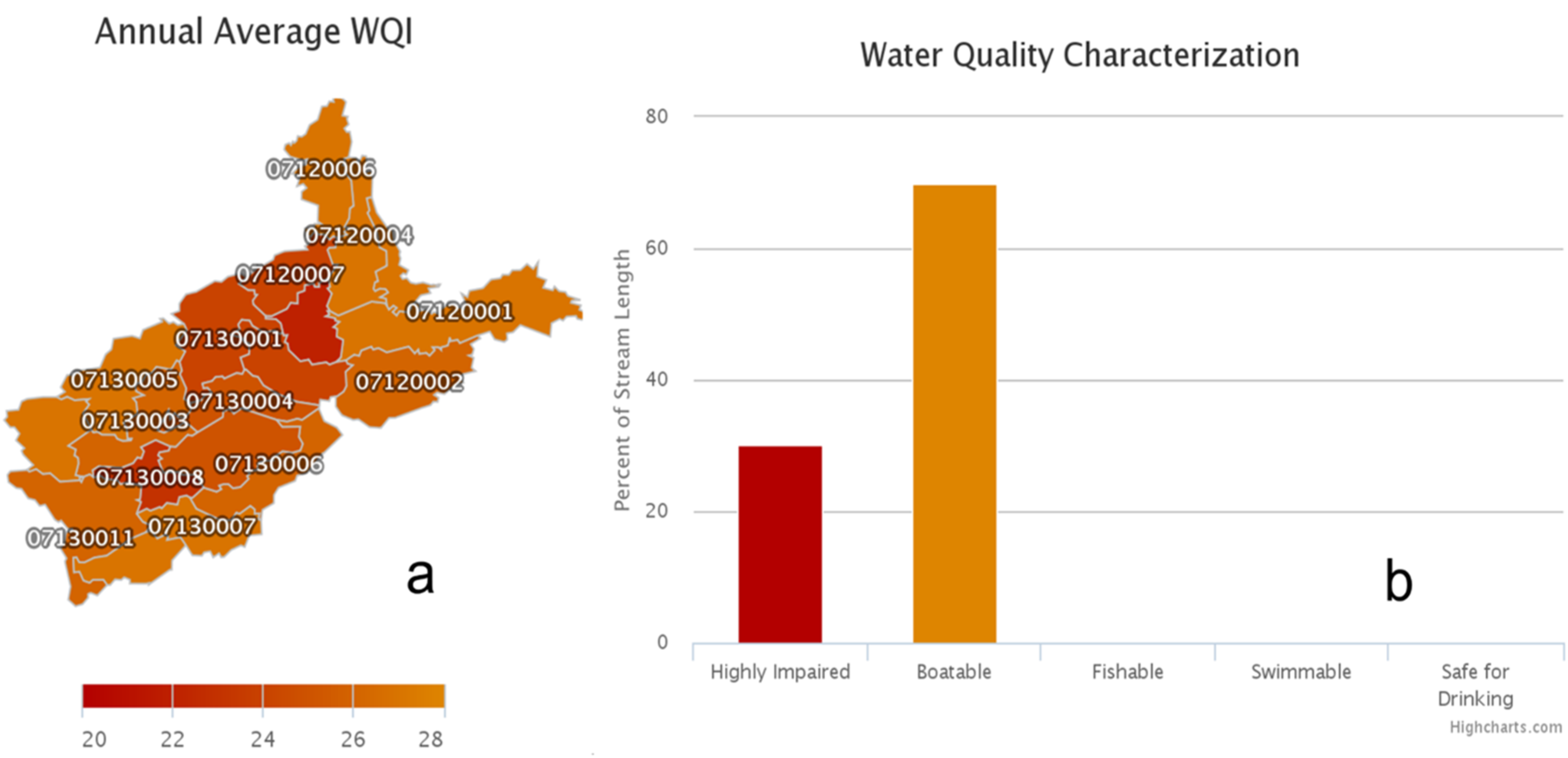
3.4.2. HAWQS Summary Charts

The SWAT model conducted by the HAWQS web interface was re-run, and it produced three summary charts using the data from 1983 to 2001. The first chart is the average monthly basin values for snowfall, surface runoff, lateral flow and water yield for each month (Figure 11). The month of May produced the highest water yield and surface runoff while the month of August produced the lowest water yield and surface runoff. Snowfall is also a major contributor in this watershed, especially in the months of December to April. The second chart shows the average monthly sediment yield for each month (Figure 12). Similar to flow, the month of May produced the highest sediment yield while the month of August produced the least. The third chart shows the average annual basin values which are the components of the hydrologic budget in the watershed (Figure 13). Figure 13 helps users understand various hydrological components in the watershed. For example, the ratios of streamflow and evapotranspiration to precipitation in this watershed are 0.47 and 0.53, respectively. In addition, the contributions of baseflow and surface runoff in this watershed are 18% and 82%.

The spatial average annual WQI in the IRW is shown in Figure 14. The WQI ranged from 20 to 28 where 12 HUC 8 watersheds are boatable and six HUC 8 watersheds are highly impaired. Highly impaired watersheds are generally distributed on the northwestern side of the watershed where agricultural activities mostly dominate. Figure 14 shows that 69% of the stream length is boatable while 30% of the stream length is impaired. The water quality of streams in the IRW is neither swimmable nor safe for drinking according to the WQI with default measurement thresholds used in the investigated watershed.

5. Conclusions

In this study, HAWQS has been demonstrated in a step-by-step scheme on the Illinois River Basin, USA. The merit of HAWQS is not only to provide delineated watershed projects for potential users, but it can also serve as an easy-to-operate and flexible tool for the complex decision-making processes. In 2014, more than 500,000 local residents in Toledo, Ohio, were facing a drinking water crisis because of the sudden degradation of water quality [38]. With the increasing population and the associated pollution caused by anthropogenic activities, requests from decision-makers for a timely analytical report with scientific guidance could be crucial. The ordinary approach of the ArcSWAT application demonstrated in this study has shown great disadvantages in major categories. With the aid of HAWQS, users can generate a preliminarily calibrated SWAT project within a few minutes by only providing the ending of a HUC number of the targeted watershed and the associated simulation period. Scientists and decision-makers can take advantage of the propounded tool on a national scale with minimum effort and without experiencing the tedious procedure of constructing a watershed project. Therefore, more resources in terms of time and financial support can be invested in other relevant issues.

References

1. Jha, M.K.; Gassman, P.W. Changes in hydrology and streamflow as predicted by a modelling experiment forced with climate models. Hydrol. Process. 2014, 28, 2772–2781. [Google Scholar] [CrossRef]
2. White, M.J.; Gambone, M.; Yen, H.; Arnold, J.G.; Harmel, R.D.; Santhi, C.; Haney, R. Regional Blue and Green Water Balances and Use by Selected Crops in the U.S. J. Am. Water Resour. Assoc. 2015, 51. [Google Scholar] [CrossRef]
3. Bai, Y.; Wagener, T.; Reed, P. A top-down framework for watershed model evaluation and selection under uncertainty. Environ. Model. Softw. 2009, 24, 901–916. [Google Scholar] [CrossRef]
4. Chou, F.N.-F.; Wu, C.-W. Determination of cost coefficients of a priority-based water allocation linear programming model—A network flow approach. Hydrol. Earth Syst. Sci. 2014, 18, 1857–1872. [Google Scholar] [CrossRef]
5. Winsemius, H.C.; Schaefli, B.; Montanari, A.; Savenije, H.H.G. On the calibration of hydrological models in ungauged basins: A framework for integrating hard and soft hydrological information. Water Resour. Res. 2009, 45, 1–15. [Google Scholar] [CrossRef]
6. Williams, J.W.; Izaurralde, R.C.; Steglich, E.M. Agricultural Policy/Environmental EXtender Model Theoretical Documentation Version 0806; Texas A&M University: College Station, TX, 2012; p. 131. [Google Scholar]
7. Bicknell, B.R.; Imhoff, J.C.; Kittle, J.L., Jr.; Donigian, A.S.; Johanson, R.C. Hydrological Simulation Program—Fortran: User’s manual for version 11; U.S. Environmental Protection Agency, National Exposure Research Laboratory: Athens, GA, USA, 1997; p. 755.
8. Arnold, J.G.; Moriasi, D.; Gassman, P.; Abbaspour, K.C.; White, M.J.; Srinivasan, R.; Santhi, C.; Harmel, R.D.; van Griensven, A.; Van Liew, M.W.; Kannan, N.; et al. SWAT: Model use, calibration, and validation. Trans. ASABE 2012, 55, 1491–1508. [Google Scholar] [CrossRef]
9. Arnold, J.G.; Youssef, M.; Yen, H.; White, M.; Sheshukov, A.; Sadeghi, A.; Moriasi, D.; Steiner, J.; Amatya, D.; Haney, E.; et al. Hydrological Processes and Model Representation. Trans. ASABE 2015, 58, 1637–1660. [Google Scholar]
10. Iowa State University, Center for Agricultural and Rural Development, SWAT Literature Database for Peer-Reviewed Journal Articles. Available online: https://www.card.iastate.edu/swat_articles/ (accessed on 19 February 2016).
11. Neitsch, S.L.; Arnold, J.G.; Kiniry, J.R.; Williams, J.R. Soil and Water Assessment Tool Theoretical Documentation Version 2009; Texas Water Resources Institute: College Station, TX, USA, 2011. [Google Scholar]
12. Moriasi, D.N.; Arnold, J.G.; Liew, M.W.V.; Bingner, R.L.; Harmel, R.D.; Veith, T.L. Model Evaluation Guidelines for Systematic Quantification of Accuracy in Watershed Simulations. Trans. ASABE 2007, 50, 885–900. [Google Scholar] [CrossRef]
13. Moriasi, D.N.; Gitau, G.W.; Pai, N.; Daggupati, P. Hydrologic and water quality models: Performance measures and criteria. Trans. ASABE 2015, 58, 1763–1785. [Google Scholar]
14. Yen, H.; Wang, X.; Fontane, D.G.; Arabi, M.; Harmel, R.D. A framework for propagation of uncertainty contributed by input data, parameterization, model structure, and calibration/validation data in watershed modeling. Environ. Model. Softw. 2014, 54. [Google Scholar] [CrossRef]
15. Abbaspour, K.C.; Yang, J.; Maximov, I.; Siber, R.; Bogner, K.; Mieleitner, J.; Zobrist, J.; Srinivasa, R. Modelling hydrology and water quality in the pre-alpine/alpine Thur watershed using SWAT. J. Hydrol. 2007, 333, 413–430. [Google Scholar] [CrossRef]
16. Yen, H.; Jeong, J.; Tseng, W-H.; Kim, M-K.; Records, R.M.; Arabi, M. Computational procedure for evaluating sampling techniques on watershed model calibration. J. Hydrol. Eng. 2015, 20. [Google Scholar] [CrossRef]
17. De, S.; Bezuglov, A. Data model for a decision support in comprehensive nutrient management in the United States. Environ. Modell. Softw. 2006, 21, 852–867. [Google Scholar] [CrossRef]
18. Miller, S.N.; Semmens, D.J.; Goodrich, D.C.; Hernandez, M.; Miller, R.C.; Kepner, W.G.; Guertin, D.P. The automated geospatial watershed assessment tool. Environ. Modell. Softw. 2007, 22, 365–377. [Google Scholar] [CrossRef]
19. Texas A&M University. Hydrologic and Water Quality System. Availalble online: https://epahawqs.tamu.edu/ (accessed on 19 February 2016).
20. Arnold, J.G.; Allen, P.M.; Bernhardt, G. A comprehensive surfacegroundwater flow model. J. Hydrol. 1993, 142, 47–69. [Google Scholar] [CrossRef]
21. Gassman, P.W.; Reyes, M.R.; Green, C.H.; Arnold, J.G. The soil and water assessment tool: Historical development, applications and future research directions. Trans. Am. Soc. Agric. Biol. Eng. 2007, 50, 1211–1250. [Google Scholar] [CrossRef]
22. Daggupati, P.; Yen, H.; White, M.J.; Srinivasan, R.; Arnold, J.G.; Keitzer, C.S.; Sowa, S.P. Impact of model development, calibration and validation decisions on hydrological simulations in West Lake Erie Basin. Hydrol. Process. 2015, 29, 5307–5320. [Google Scholar] [CrossRef]
23. Texas A&M University. Soil and Water Assessment Tool. ArcSWAT Interface and documentations. Available online: http://swat.tamu.edu/software/arcswat/ (accessed on 19 February 2016).
24. University of Illinois at Urbana-Champaign. Atmosphere Deposition—National Atmospheric Deposition Program (NADP). Available online: http://nadp.sws.uiuc.edu/ (accessed on 19 February 2016).
25. United States Department of Agriculture, Natural Resources Conservation Practices, Climate—Parameter-elevation Regressions on Independent Slopes Model (PRISM). Available online: http://www.wcc.nrcs.usda.gov/climate/prism.html (accessed on 19 February 2016).
26. United States Geological Survey, Land Use (non-agricultural)—National Land Cover Database (NLCD). Available online: http://www.mrlc.gov/nlcd06_data.php (accessed on 19 February 2016).
27. United States Department of Agriculture; National Agricultural Statistics Service (NASS). Land Use—Cropland Data Layer (Agricultural). Available online: http://nassgeodata.gmu.edu/CropScape/ (accessed on 19 February 2016).
28. United States Corps pf Engineers, Reservoirs—National Inventory of Dams (NID). Available online: http://nid.usace.army.mil/cm_apex/f?p=838:5:0::NO (accessed on 19 February 2016).
29. United States Geological Survey, River Discharge Data. Available online: http://waterdata.usgs.gov/nwis (accessed on 19 February 2016).
30. United States Department of Agriculture, Natural Resources Conservation Practices, State Soil Geographic Data. Available online: http://sdmdataaccess.nrcs.usda.gov/ (accessed on 19 February 2016).
31. United States Geological Survey, Global Data Explorer. Available online: http://gdex.cr.usgs.gov/gdex/ (accessed on 19 February 2016).
32. United States Geological Survey, Water Usage Data. Available online: http://water.usgs.gov/watuse/data/ (accessed on 19 February 2016).
33. Michael, W.; Harmel, J.; Daren, R.; Arnold, J.G.; Williams, J.R. SWAT Check: A screening tool to assist users in the identification of potential model application problems. J. Environ. Qual. 2014, 43, 208–214. [Google Scholar]
34. United State Environmental Protection Agency (USEPA). Environmental Impact and Benefits Assessment for Final Effluent Guidelines and Standards for the Construction and Development Category; Office of Water: Washington, DC, USA, 2009. [Google Scholar]
35. Illinois Environmental Protection Agency. Water Quality for Citizens. Available online: http://www.epa.illinois.gov/ (accessed on 19 February 2016).
36. Daggupati, P.; Pai, N.; Ale, S.; Douglas-Mankin, K.R.; Zeckoski, R.W.; Jeong, J.; Parajuli, P.B.; Saraswat, D.; Youssef, M.A. A recommended calibration and validation strategy for hydrologic and water quality models. Trans. ASABE 2015, 58, 1705–1719. [Google Scholar]
37. Nash, J.E.; Sutcliffe, J.V. River flow forecasting through conceptual models part I—A discussion of principles. J. Hydrol. 1970, 10, 282–290. [Google Scholar] [CrossRef]
38. Dungjen, T.; Patch, D. Toledo-area Water Advisory Expected to Continue through Sunday as Leaders Await Tests. The Blade. Available online: http://www.toledoblade.com/local/2014/08/02/City-of-Toledo-issues-do-no-drink-water-advisery.html (accessed on 19 February 2016).
Figure 1. Organogram of the HAWQS operational framework.
Water 08 00164 g001
Figure 2. Initialization—watershed selection.
Water 08 00164 g002
Figure 3. Initialization—watershed confirmation.
Water 08 00164 g003
Figure 4. Customization: (i) HRU settings; (ii) basin level settings; and (iii) subbasin level settings.
Water 08 00164 g004
Figure 5. Output management: (i) reach/subbasin/HRU parameters; (ii) HRU output variables; and (iii) execution of the SWAT project.
Water 08 00164 g005
Figure 6. Output demonstration: (i) output reach data; (ii) output summary charts; (iii) download input.std and output.std files; (iv) perform SWAT-Check; and (v) water quality index calculation.
Water 08 00164 g006
Figure 7. Hydrological outputs (process-based diagram) generated by SWAT-Check (diagrams for sediment and nutrient processes are also available in SWAT-Check [2].
Water 08 00164 g007
Figure 8. Units and ranges of Water Quality Index (WQI) for eight water quality variables.
Water 08 00164 g008
Figure 9. Location of the Illinois River Basin (IRW).
Water 08 00164 g009
Figure 10. Time series comparisons between observed and predicted flow, sediment and TN for calibration and validation periods for the Illinois River Basin. (a) Streamflow; (b) Sediment; (c) Total Nitrogen.
Water 08 00164 g010
Figure 11. Average monthly basin values for snowfall, surface runoff, lateral flow and water yield for each month for the Illinois River Basin.
Water 08 00164 g011
Figure 12. Average monthly sediment yield for the Illinois River Basin.
Water 08 00164 g012
Figure 13. Average annual basin values for the hydrologic components for the Illinois River Basin.
Water 08 00164 g013
Figure 14. Water quality characterization in IRW.
Water 08 00164 g014