A Two-Step Approach for Analytical Optimal Hedging with Two Triggers

Abstract

Hedging is widely used to mitigate severe water shortages in the operation of reservoirs during droughts. Rationing is usually instituted with one hedging policy, which is based only on one trigger, i.e., initial storage level or current water availability. It may perform poorly in balancing the benefits of a release during the current period versus those of carryover storage during future droughts. This study proposes a novel hedging rule to improve the efficiency of a reservoir operated to supply water, in which, based on two triggers, hedging is initiated with three different hedging sub-rules through a two-step approach. In the first step, the sub-rule is triggered based on the relationship between the initial reservoir storage level and the level of the target rule curve or the firm rule curve at the end of the current period. This step is mainly concerned with increasing the water level or not in the current period. Hedging is then triggered under the sub-rule based on current water availability in the second step, in which the trigger implicitly considers both initial and ending reservoir storage levels in the current period. Moreover, the amount of hedging is analytically derived based on the Karush–Kuhn–Tucker (KKT) conditions. In addition, the hedging parameters are optimized using the improved particle swarm optimization (IPSO) algorithm coupled with a rule-based simulation. A single water-supply reservoir located in Hubei Province in central China is selected as a case study. The operation results show that the proposed rule is reasonable and significantly improves the reservoir operation performance for both long-term and critical periods relative to other operation policies, such as the standard operating policy (SOP) and the most commonly used hedging rules.

1. Introduction

The occurrence of severe and frequent droughts has highlighted the need to improve reservoir operation rules to better aid water supply operators in coping with the risk of dramatic water supply shortfalls [1]. Hedging rules are quite useful in mitigating the potential negative impacts during future droughts because they generate smaller deficits by curtailing current delivery even when there is enough water to meet demand [2,3,4,5,6,7,8]. A good hedging rule can effectively reduce a very high-percentage single-period water shortage. However, unnecessary hedging increases more frequent small shortages that decrease the reliability of the water supply [9].

Defining appropriate hedging rules is typically a complex decision-making process involving many decision-makers, considerable risk, the presence of uncertain future inflows and nonlinear economic benefits associated with the released water. Hedging has been and continues to be the subject of numerous research works since Bower’s study during the Harvard Water Program [3]. This attention is due to the essential benefits arising from reservoir operation in combination with the reduction of natural risks. Recent decades have witnessed the development of a plethora of hedging rules of varying degrees of complexity and sophistication. Some aspects of hedging rules that have been addressed include the triggers of the onset and termination of water restrictions, the percentage of water rationing (hedging factor), the effects of hedging on reservoir performance, analytical hedging rules, rationality of hedging, inflow uncertainty, the effects of reservoir evaporation on hedging, and the optimal conditions for hedging rules [6,7,9,10]. Most recently, hedging has been addressed in the context of economic water operation [4,5,8]. Although many aspects of hedging have been extensively investigated, the appropriate selection of the triggers of the onset and termination of water rationing has not been thoroughly studied.

Generally, the supply of water increases when water availability increases at any particular instant in time. In this regard, water storage [11,12,13,14,15,16] and water availability (defined as storage plus inflow [2,7,17,18,19]) are the two most commonly used triggers. Shih and ReVelle [18] argued that using storage augmented by expected inflows results in potentially more reasonable behavior. However, Shiau and Lee [9] found that hedging cannot be initiated earlier for an impending severe shortage based only on water availability. Based on these two triggers, the same hedging factor would be obtained for the same current water availability, which is not necessarily true under every circumstance. The supply–demand relationship, in terms of potential shortages in future periods, is an essential factor for determining whether hedging should be implemented. More specifically, the relationship between the initial storage level and the level of the target rule curve and/or firm rule curve has a significant effect on hedging. For example, when the initial storage level is below the target storage level, reservoir operators tend to store water to bring the storage level up to the target storage level, which is not the case when the initial storage level is above the target storage level.

Based on this relationship, Shiau and Lee [9] derived an optimal hedging rule based on potential shortage conditions within a specific future “lead-time”, in which monthly decile inflows are suggested as a substitute for predicted future inflows because the future inflows cannot be known exactly. Taghian et al. [20] developed a new hedging method in which the relationships between the reservoir storage level (including both the initial and ending storage levels) and the monthly target and firm rule curves were used as triggers. Depending on the heights of the initial and ending reservoir storage levels, a different fraction of the demand is released. Furthermore, Neelakantan and Pundarikanthan [13] found that triggering mechanisms are generally based on the water storage in a reservoirs, rainfall, stream flow levels, groundwater levels, sea water intrusion rates and drought indicators, such as the Palmer index. In addition, Zeng et al. [21] derived release rules for an individual reservoir in a parallel reservoir system with joint water demand. In these rules, the total water availability of reservoir system determined the implementation of system hedging, but the water availability of the individual reservoirs decided the respective levels of water supply. Notwithstanding the progress in defining hedging rules discussed above, we share the concern expressed in the literature that the mechanism that triggers supply reduction based only on water storage or water availability has certain limitations that necessitate the development of a new trigger. The current trigger mechanism is limited by the fact that reservoir inflows cannot be exactly known and by the fact that the relationship between potential water shortage and water availability is not fully considered.

Following Taghian et al. [20], this paper developed an analytical optimal hedging rule with two triggers to improve the above-mentioned limitations by adopting a two-step approach for hedging to implicitly incorporate the relationship between water availability and water shortage. This hedging rule relates the release to both the water availability during the current period and the level of the initial storage. Therefore, instead of defining only one hedging rule for reservoir operation, the proposed rule, which consists of three hedging sub-rules, is derived based on Karush–Kuhn–Tucker conditions (also known as Kuhn–Tucker or KKT conditions, see Bazaraa et al. [22] for details). The relationship between the initial storage level and the levels of the rule curves at the end of the current period is also used as a trigger to determine which sub-rule is used to guide the reservoir operation. The current water availability is used to decide when to start and end hedging under each sub-rule. In addition, an improved particle swarm optimization (IPSO) algorithm coupled with the rule-based simulation model is established to obtain the optimal hedging parameters. Finally, the Xujiahe reservoir, located in central China, is taken as a case study to verify the reasonableness and efficiency of the proposed rule.

2. Methods

The methods in this paper are organized as follows: In Section 2.1, an optimal hedging rule with two triggers is analytically derived via a two-step approach for hedging. In Section 2.2, the optimization-simulation model is applied to optimize the parameters of the derived optimal hedging for long-term operation.

2.1. Analytical Optimal Hedging Rule with Two Triggers (AOHR-TT)

The key outcome of Taghian et al. [20], referred to as Taghian’s method in this paper, was the hedging policy developed for different reservoir zones coupled with a linear programming (LP) model. Under this policy, different rationing factors, i.e., 1, α₁ and α₂ (0 < α₂ < α₁ < 1), are assigned to the expected demand, from the upper to the lower zones, when the initial and ending reservoir storage levels during the current period are located in the same zone. For levels that vary between zones, the rationing factor is between the corresponding values of the zones to keep the end-of-period storage level as close to the rule curves as possible. This policy, adopted in this paper, is illustrated in Figure 1.

Figure 1. The hedging policy for different reservoir zones based on the initial storage and ending storage levels.

Figure 1. The hedging policy for different reservoir zones based on the initial storage and ending storage levels.

In this paper, Taghian’s method has been modified and three improvements have been made. First, a non-linear objective function with the exponent m (m > 1) is used to replace the linear objective function suggested by Taghian et al. [20] to represent the characteristics of “hedging”. Second, by translating the relationship between the ending storage level and the rule curve levels to the constraints for a nonlinear objective, an analytical optimal hedging rule is derived to replace the rule in Taghian’s method. This improvement provides easier operation and useful information for analyzing the effects of hedging. Third, the penalties corresponding to reservoir zones and water shortage are employed as decision variables in the optimization model rather than pre-determined values. This method better reflects the relationship between the weighting of storage benefits and release benefits and has an important effect on the hedging.

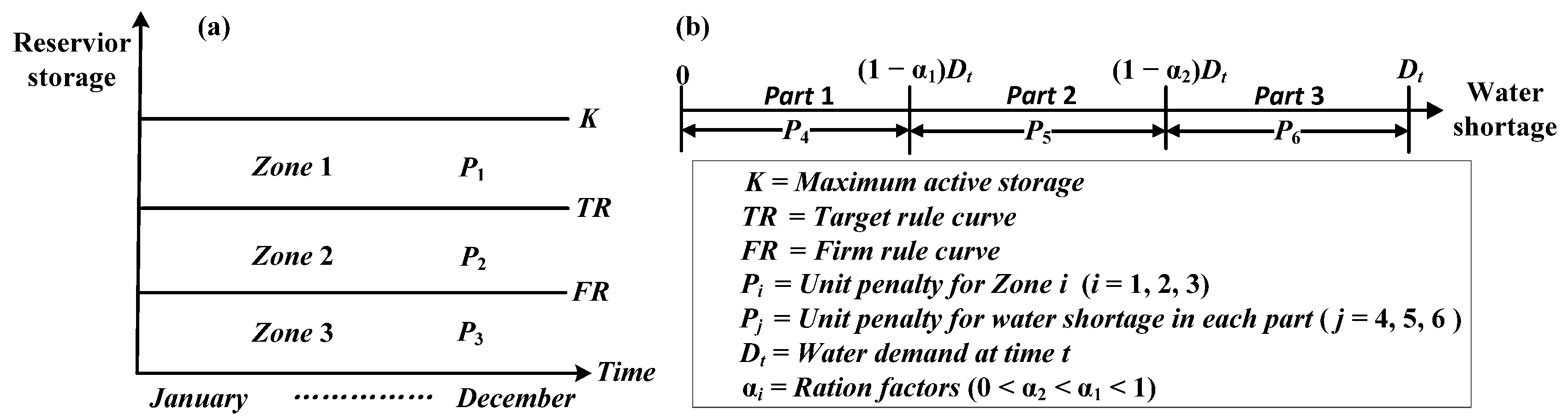
2.1.1. Mathematical Programming Model for the AOHR-TT

The reservoir operation benefits in a two-period model consist of two parts, i.e., the current release benefits and the carryover reservoir storage benefits, which are often expressed as ‘‘loss’’ or ‘‘penalty’’ functions [4]. In this paper, the former is expressed as the mth power of deviations from the demand targets, whereas the latter is expressed as the mth power of deviations from the reservoir storage targets (i.e., deviations from the rule curves), which are similar to the functions in Taghian’s method. The objective function of the reservoir operation includes minimization of the weighted sum of loss functions (i.e., deviations from the targets) (Equation (1)), water balance equations (Equations (2)–(5)) and constraints on the deviations from the targets (Equations (6) and (7)), which can be generalized into the following mathematical programming model:

$$\underset{V{R}_t,V{D}_t}{\min }f=P_i\cdot V{R}_t^m+P_j\cdot V{D}_t^m$$

(1)

$$s.t.S_t=S_{t-1}+R{I}_t-R_t-L{S}_t-S{U}_t$$

(2)

$$S_t=R{C}_t^{*}\pm V{R}_t$$

(3)

$$R_t=D_t-V{D}_t$$

(4)

$$W{A}_t=S_{t-1}+R{I}_t-L{S}_t$$

(5)

$$V{R}_{lt}\le V{R}_t\le V{R}_{ut}$$

(6)

$$V{D}_{lt}\le V{D}_t\le V{D}_{ut}$$

(7)

where $V{D}_t$ is the deviation from the projected water supply demand; $V{R}_t$ is the storage deviation from the rule curve; $P_i$ (i = 1, 2, 3) and $P_j$ (j = 4, 5, 6) are the unit penalties for the $V{R}_t$ located in Zone i and $V{D}_t$ located in Part j, respectively, as shown in Figure 2; m is an exponent of loss function (m > 1); $S_{t-1}$ and $S_t$ are the water stored in the reservoir at the start and end of time t, respectively; $L{S}_t$ is the evaporation and seepage loss at time t; $S{U}_t$ is the water spilled at time t; $R{C}_t^{*}$ is $T{R}_t$ or $F{R}_t$, representing the target rule curve or firm rule curve, respectively, at the end of time t; $R_t$ is the reservoir release at time t; $D_t$ is the projected demand at time t (demand target); $W{A}_t$ is the water availability at time t; $R{\text{I}}_t$ is the reservoir inflow at time t; $V{R}_{ut}$ and $V{R}_{lt}$ are the upper and lower bounds for $V{R}_t$, respectively; and $V{D}_{ut}$ and $V{D}_{lt}$ are the upper and lower bounds for $V{D}_t$, respectively. $V{R}_{ut}$, $V{R}_{lt}$, $V{D}_{ut}$, and $V{D}_{lt}$ can be obtained from the relationship between $S_t$ and $T{R}_t$ (or $F{R}_t$) and the hedging policy in Figure 1. $T{R}_t$, $F{R}_t$, ${\alpha }_i$ (i = 1, 2), $P_i$ (j = 1, 2, 3) and $P_j$ (j = 4, 5, 6) can be obtained based on optimization or expert knowledge. In this study, the active storage levels are obtained by subtracting the dead storage level from $T{R}_t$, $F{R}_t$, $S_t$, and $S_{t-1}$.

Figure 2. The penalty structure: (a) penalty structure based on reservoir zone and (b) penalty structure for water shortage based on demand during rationing.

Figure 2. The penalty structure: (a) penalty structure based on reservoir zone and (b) penalty structure for water shortage based on demand during rationing.

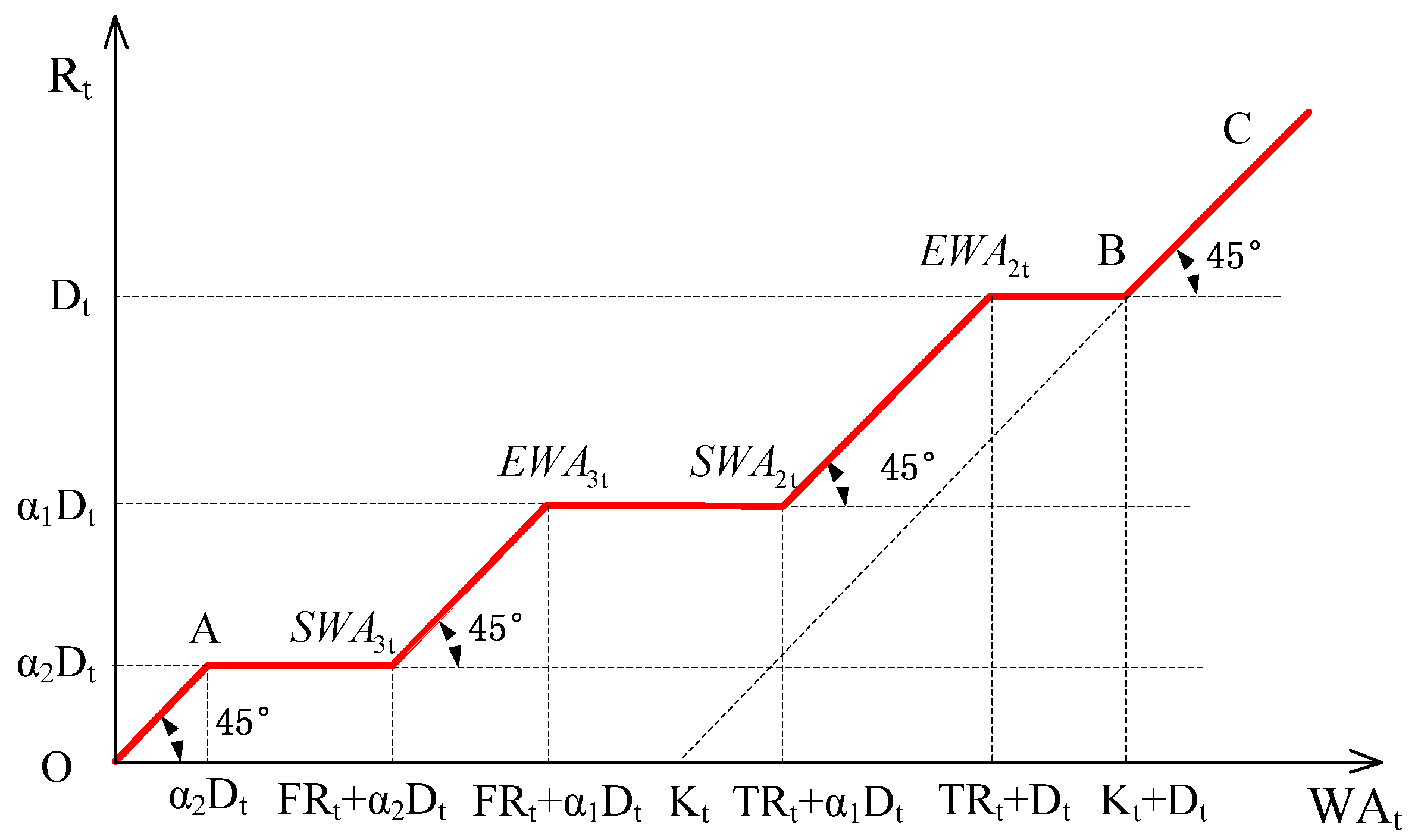
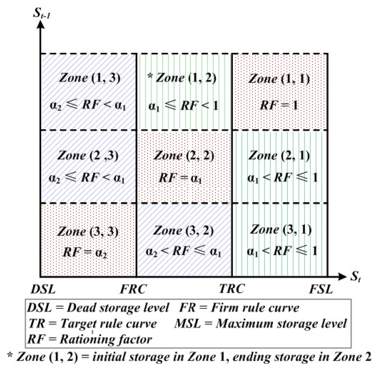
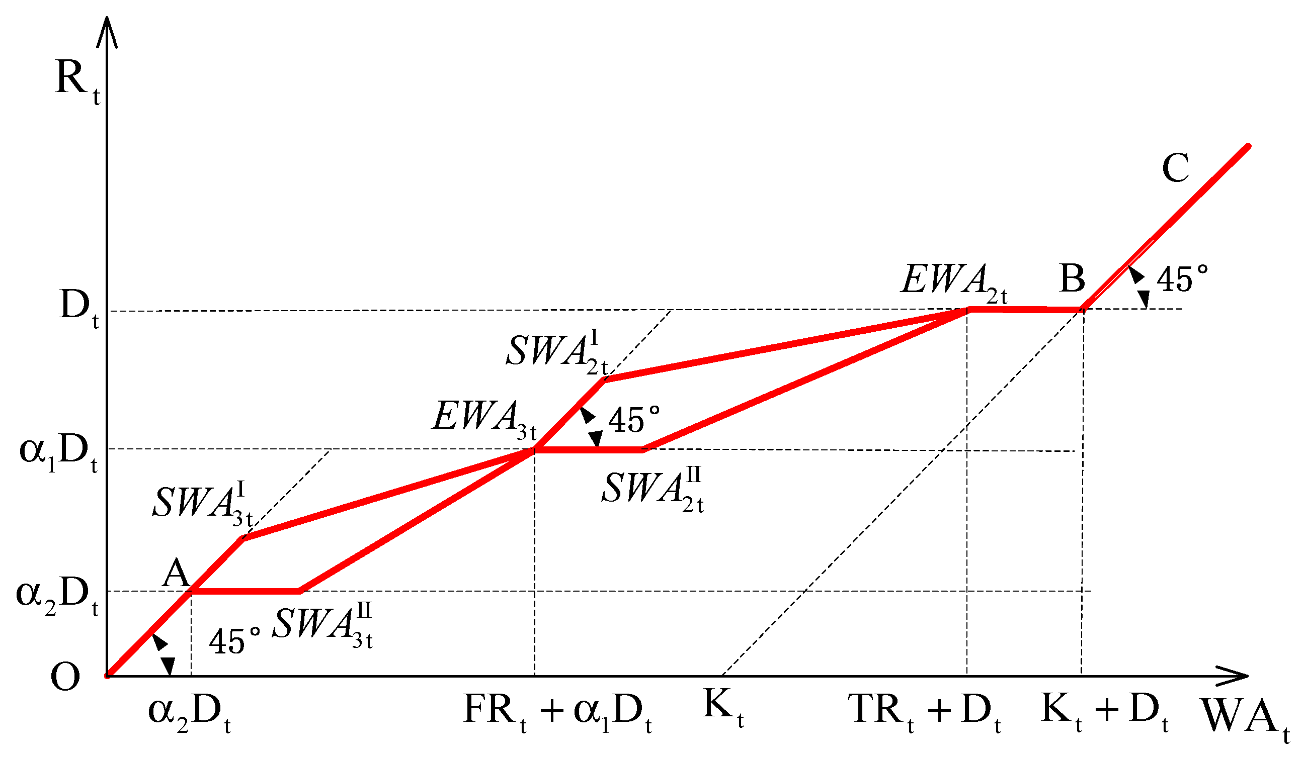
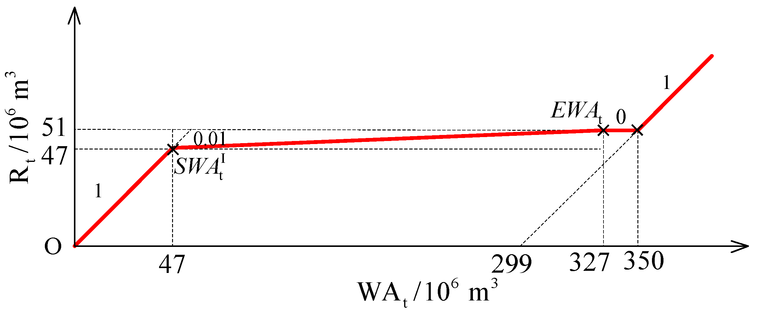
2.1.2. Model Solution and Analysis

Assuming that the minimum water release requirement is equal to the α₂ proportion of the demand target, the proposed rule will be not applicable if the water availability is less than the minimum demand, i.e., $W{A}_t<D_t\cdot {\alpha }_2$, because the minimum water release constraint is not satisfied. When water availability exceeds the sum of the demand target and the carryover storage target, i.e., $W{A}_t>D_t+T{R}_t$, hedging is not necessary because the water stored in the reservoir is sufficient to satisfy both the water release and the carryover storage targets [5]. In these cases, the standard operating policy (SOP) is used to guide the reservoir operation. The level of water shortage located in Part 3 in Figure 2 means the implementation of SOP under which $P_j$ (j = 6) has no effect on hedging and can thus be set to a large value to punish the loss functions for avoiding a water shortage in Part 3.

A two-step approach for hedging based on two triggers is used to establish the hedging rule. In the first step, the sub-rule of the hedging rule is triggered based on the state of $S_{t-1}$ (i.e., the relationship between the initial reservoir storage level and the level of the ideal rule curve at the end of the current period). This step implicitly incorporates potential water shortages in future periods and determines whether the amount of stored water should be increased. Hedging under the sub-rule is then triggered based on current water availability in the second step. Different from the commonly used trigger mechanism for hedging only making decisions via the state of $S_{t-1}$, the second-step triggering mechanism implicitly considers both the initial and ending storage of reservoir in the current period based on the hedging policy in Figure 2.

To facilitate the analysis in this paper, the reservoir storage is divided into three zones based on the rule curves, as shown in Figure 2. Thus, $S_{t-1}$ can be located in Zone 1, Zone 2, or Zone 3, corresponding to normal, drought, or severe drought conditions, respectively. Based on the different $S_{t-1}$ conditions, three hedging sub-rules of the analytical optimal hedging rule with two triggers (AOHR-TT) are analytically derived below:

(1)

Rule 1: $S_{t-1}$ is located in Zone 1, which corresponds to normal conditions, i.e., $T{R}_t\le S_{t-1}\le K_t$

According to the operation policy defined in Figure 1 for $S_{t-1}$, there are three possible cases for $S_t$, i.e., $S_t$ can be located in Zone 1, Zone 2, or Zone 3. When $S_t$ is located in Zone 1, the constraints for $V{R}_t$ and $V{D}_t$ (i.e., Equations (6) and (7)) can be obtained using Equation (3) and Equation (4) based on the zone constraints for the $S_t$ and RF of Zone (1, 1) (Figure 1), respectively. By substituting Equations (3) and (4) into Equation (5), the water balance equation for $V{R}_t$ and $V{D}_t$ can be derived. The resulting inequality constraints and equality constraints for $V{R}_t$ and $V{D}_t$ constitute the constraints for the case where $S_t$ is located in Zone 1. That is,

$$s.t.\{\begin{array}{l}V{D}_t=0\\ 0\le V{R}_t\le K_t-T{R}_t\\ V{R}_t=W{A}_t-T{R}_t-D_t\end{array}$$

(8)

Similarly, the constraints for the case where $S_t$ is located in Zone 2 and Zone 3 can be obtained, as expressed in Equations (9) and (10), respectively.

$$s.t.\{\begin{array}{l}0<V{D}_t\le (1-{\alpha }_1)D_t\\ 0<V{R}_t\le T{R}_t-F{R}_t\\ -V{R}_t-V{D}_t=W{A}_t-T{R}_t-D_t\end{array}$$

(9)

$$s.t.\{\begin{array}{l}0<V{D}_t\le ({\alpha }_1-{\alpha }_2)D_t\\ 0<V{R}_t\le F{R}_t\\ -V{R}_t-V{D}_t=W{A}_t-F{R}_t-{\alpha }_1{D}_t\end{array}$$

(10)

In this paper, Karush–Kuhn–Tucker (KKT) conditions are used to solve the mathematical programming model comprising the objective function (i.e., Equation (1)) and the constraints for $V{R}_t$ and $V{D}_t$ that correspond to the cases where $S_t$ is located in Zone 1, Zone 2, and Zone 3 (i.e., Equations (8)–(10), respectively). The optimal water supply for Rule 1 can be derived as follows:

$$R_t^{\text{I}}=\{\begin{array}{lll}W{A}_t,& & W{A}_t<{\alpha }_2{D}_t\\ R_{3t}^{\prime },& \hfill {\alpha }_2{D}_t\le & W{A}_t<SW{A}_{3t}\\ R_{3t}^{*},& SW{A}_{3t}\le & W{A}_t<EW{A}_{3t}\\ R_{2t}^{\prime },& EW{A}_{3t}\le & W{A}_t<SW{A}_{2t}\\ R_{2t}^{*},& SW{A}_{2t}\le & W{A}_t<EW{A}_{2t}\\ D_t,& & W{A}_t\ge EW{A}_{2t}\end{array}$$

(11)

where $R_t^{\text{I}}$ is the optimal water supply for Rule 1 and $SW{A}_{it}$ and $EW{A}_{it}$ are the starting water availability (SWA) and ending water availability (EWA) for hedging, respectively, and correspond to the case where $S_t$ is located in Zone i (i = 2, 3), respectively. The term $EW{A}_{it}$ can be expressed as Equation (12), and the terms $R_{3t}^{\prime }$, $R_{2t}^{\prime }$, $R_{3t}^{*}$ and $R_{2t}^{*}$ can be expressed as Equations (13)–(16), respectively.

$$\{\begin{array}{l}EW{A}_{3t}=F{R}_t+{\alpha }_1{D}_t\\ EW{A}_{2t}=T{R}_t+D_t\end{array}$$

(12)

$$R_{3t}^{\prime }=\{\begin{array}{lll}W{A}_t,& {\alpha }_2{D}_t\le W{A}_t<SW{A}_{3t}^{\text{I}},& if{\eta }_{3t}\ge 1\\ {\alpha }_2{D}_t,& {\alpha }_2{D}_t\le W{A}_t<SW{A}_{3t}^{\text{II}},& if{\eta }_{3t}<1\end{array}$$

(13)

$$R_{2t}^{\prime }=\{\begin{array}{lll}W{A}_t-F{R}_t,& EW{A}_{3t}\le W{A}_t<SW{A}_{2t}^{\text{I}},& if{\eta }_{2t}\ge 1\\ {\alpha }_1{D}_t,& EW{A}_{3t}\le W{A}_t<SW{A}_{2t}^{\text{II}},& if{\eta }_{2t}<1\end{array}$$

(14)

$$R_{3t}^{*}=\frac{{\eta }_{3}W{A}_t}{{\eta }_3+1}+\frac{{\alpha }_1{D}_t}{{\eta }_3+1}-\frac{{\eta }_{3}F{R}_t}{{\eta }_3+1}$$

(15)

$$R_{2t}^{*}=\frac{{\eta }_{2}W{A}_t}{{\eta }_2+1}+\frac{D_t}{{\eta }_2+1}-\frac{{\eta }_{2}T{R}_t}{{\eta }_2+1}$$

(16)

In Equations (13) and (14), $SW{A}_{it}^{\text{I}}$ and $SW{A}_{it}^{\text{II}}$ are the two types of $SW{A}_{it}$ (i = 2, 3), which are expressed as Equation (17). In Equations (15) and (16), ${\mathsf{\eta }}_2$ (or ${\mathsf{\eta }}_3$) is the weighting ratio between the penalty for $S_t$ located in Zone 2 (or 3) and the penalty for water shortage located in Part 1 (or 2). These terms can be expressed as Equation (18). The parameter ${\mathsf{\eta }}_{it}$ is used to detect the type of $SW{A}_{it}$ (i = 2, 3) and is defined as Equation (19).

$$\{\begin{array}{l}SW{A}_{3t}^{\text{I}}={\alpha }_1{D}_t-{\eta }_{3}F{R}_t\\ SW{A}_{3t}^{\text{II}}=F{R}_t+{\alpha }_2{D}_t+\frac{\left({\alpha }_2-{\alpha }_1\right)D_t}{{\eta }_3}\\ SW{A}_{2t}^{\text{I}}=D_t+F{R}_t+{\eta }_2(F{R}_t-T{R}_t)\\ SW{A}_{2t}^{\text{II}}=T{R}_t+{\alpha }_1{D}_t+\frac{\left({\alpha }_1-1\right)D_t}{{\eta }_2}\end{array}$$

(17)

$$\{\begin{array}{l}{\eta }_2={\left(\frac{P_2}{P_4}\right)}^{\frac{1}{m-1}}\\ {\eta }_3={\left(\frac{P_3}{P_5}\right)}^{\frac{1}{m-1}}\end{array}$$

(18)

$$\{\begin{array}{l}{\eta }_{2t}=(\frac{D_t}{T{R}_t-F{R}_t})(\frac{1-{\alpha }_1}{{\eta }_2})\\ {\eta }_{3t}=(\frac{D_t}{F{R}_t})(\frac{{\alpha }_1-{\alpha }_2}{{\eta }_3})\end{array}$$

(19)

The derived optimal hedging policy for Rule 1 (i.e., Equation (11)) is illustrated in Figure 3. In the figure, the slope of the linear hedging from $SW{A}_{it}$ to $EW{A}_{it}$ varies with the range in water availability, and the release exhibits piecewise linear characteristics. Two types of SWA are included in the hedging policy for each EWA, e.g., $SW{A}_{3t}^{\text{I}}$ and $SW{A}_{3t}^{\text{II}}$ correspond to $EW{A}_{3t}$. If ${\mathsf{\eta }}_{2t}>1$ (or ${\mathsf{\eta }}_{3t}>1$), $SW{A}_{2t}^{\text{I}}$ (or $SW{A}_{3t}^{\text{I}}$) would be identified as the type of $SW{A}_{2t}$ (or $SW{A}_{3t}$), and the increasing rate of release would be the same as that of the water availability within the range bounded by $EW{A}_{3t}$ (or A) and $SW{A}_{2t}^{\text{I}}$ (or $SW{A}_{3t}^{\text{I}}$) due to the relatively high weighting of the release benefit. In contrast, if ${\eta }_{2t}<1$ (or ${\eta }_{3t}<1$), $SW{A}_{2t}^{\text{I}}$ (or $SW{A}_{3t}^{\text{I}}$) would be replaced by $SW{A}_{2t}^{\text{II}}$ (or $SW{A}_{3t}^{\text{II}}$), and the release would be fixed and less than that for ${\mathsf{\eta }}_{2t}>1$ (or ${\mathsf{\eta }}_{3t}>1$) within the range bounded by $EW{A}_{3t}$ (or A) and $SW{A}_{2t}^{\text{II}}$ (or $SW{A}_{3t}^{\text{II}}$) due to the relatively low weighting of the release benefit (or, alternatively, the relatively high weighting of the storage benefit). In other words, the marginal benefit of release in the range of $EW{A}_{3t}<W{A}_t\le SW{A}_{2t}^{\text{I}}$ (or $A<W{A}_t\le SW{A}_{3t}^{\text{I}}$) for ${\mathsf{\eta }}_{2t}>1$ (or ${\mathsf{\eta }}_{3t}>1$) is higher than that in the range of $EW{A}_{3t}<W{A}_t\le SW{A}_{2t}^{\text{II}}$ (or $A<W{A}_t\le SW{A}_{3t}^{\text{II}}$) for ${\mathsf{\eta }}_{2t}<1$ (or ${\mathsf{\eta }}_{3t}<1$).

If the ${\alpha }_1$ proportion of the demand target (i.e., ${\alpha }_1{D}_t$) is large, a majority of water demand will be met when $W{A}_t$ reaches $EW{A}_{3t}$. Thus, when $W{A}_t$ ranges between $SW{A}_{2t}$ and $EW{A}_{2t}$, the marginal benefit of a release decreases, which results in a lower slope in the linear hedging than that within the range of $SW{A}_{3t}\le W{A}_t\le EW{A}_{3t}$. This process ensures that the storage in a reservoir is as close to the storage target (i.e., target rule curve) as possible. In contrast, if ${\alpha }_1{D}_t$ is small, the degree of water deficits will remain severe even when $W{A}_t$ reaches $EW{A}_{3t}$. Therefore, when $W{A}_t$ ranges between $SW{A}_{2t}$ and $EW{A}_{2t}$, the weighting of the release benefit (or the marginal benefit of a release) increases, which results in a higher slope in the linear hedging from $SW{A}_{2t}$ to $EW{A}_{2t}$ than that from $SW{A}_{3t}$ to $EW{A}_{3t}$. This process allows the release of as much water as possible to meet the demand. If the weighting of the release benefit within the range of $SW{A}_{2t}$ to $EW{A}_{2t}$ is taken to be equal to that within the range of $SW{A}_{3t}$ to $EW{A}_{3t}$ by assigning some value to ${\alpha }_1{D}_t$, the slope of the linear hedging within these two ranges will be the same. Thus, the degree to which $W{A}_t$ within the range of $SW{A}_{2t}$ to $EW{A}_{2t}$ affects the release benefit and the reservoir storage benefit is same as that within the range of $SW{A}_{3t}$ to $EW{A}_{3t}$.

Figure 3. The derived optimal hedging policy for Rule 1.

Figure 3. The derived optimal hedging policy for Rule 1.

Because water availability within the range bounded by $EW{A}_{3t}$ and $SW{A}_{2t}^{\text{II}}$ is more than that bounded by A and $SW{A}_{3t}^{\text{II}}$, more water is released in the range of $EW{A}_{3t}$ to $SW{A}_{2t}^{\text{II}}$. When $W{A}_t$ exceeds $EW{A}_{2t}$, the storage target ($T{R}_t$) is reached, and the water supply is no longer restricted, i.e., the demand target is fully satisfied. Specially, a $W{A}_t$ equal to B means the maximum active storage capacity has been reached. Then, as $W{A}_t$ increases further, spilling occurs and increases at a rate identical to that of $W{A}_t$.

(2)

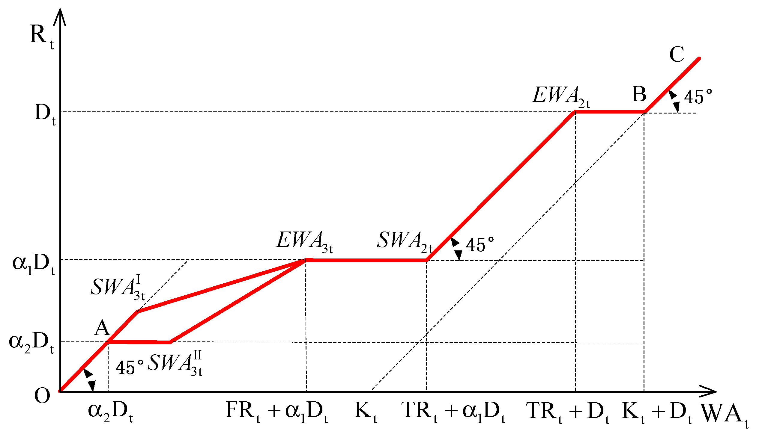
Rule 2: $S_{t-1}$ is located in Zone 2, which corresponds to drought conditions, i.e., $F{R}_t\le S_{t-1}<T{R}_t$

Similar to Rule 1, in accordance with KKT conditions, the optimal water supply for Rule 2 can be expressed as follows:

$$R_t^{\text{II}}=\{\begin{array}{lll}W{A}_t,& & W{A}_t<{\alpha }_2{D}_t\\ R_{3t}^{\prime },& \hfill {\alpha }_2{D}_t\le & W{A}_t<SW{A}_{3t}\\ R_{3t}^{*},& \hfill SW{A}_{3t}\le & W{A}_t<EW{A}_{3t}\\ {\alpha }_1{D}_t,& \hfill EW{A}_{3t}\le & W{A}_t<T{R}_t+{\alpha }_1{D}_t\\ W{A}_t-T{R}_t,& \hfill T{R}_t+{\alpha }_1{D}_t\le & W{A}_t<T{R}_t+D_t\\ D_t,& & W{A}_t\ge T{R}_t+D_t\end{array}$$

(20)

where $R_t^{\text{II}}$ is the optimal water supply for Rule 2. The terms $R_{3t}^{\prime }$ and $R_{3t}^{*}$ can be expressed as Equations (21) and (22), respectively.

$$R_{3t}^{\prime }=\{\begin{array}{lll}W{A}_t,& {\alpha }_2{D}_t\le W{A}_t<SW{A}_{3t}^{\text{I}},& if{\eta }_{3t}\ge 1\\ {\alpha }_2{D}_t,& {\alpha }_2{D}_t\le W{A}_t<SW{A}_{3t}^{\text{II}},& if{\eta }_{3t}<1\end{array}$$

(21)

$$R_{3t}^{*}=\frac{{\eta }_{3}W{A}_t}{{\eta }_3+1}+\frac{{\alpha }_1{D}_t}{{\eta }_3+1}-\frac{{\eta }_{3}F{R}_t}{{\eta }_3+1}$$

(22)

Equation (20) is illustrated in Figure 4, which differs from Figure 3 within the range bounded by $EW{A}_{3t}$ and $EW{A}_{2t}$. According to Equation (17) and Figure 4, $SW{A}_{2t}$ in Figure 4 is greater than $SW{A}_{2t}^{\text{II}}$ in Figure 3. Because the value of $S_{t-1}$ in Rule 2 is below the level of the target rule curve, more water is retained to keep the storage level as close to the storage target as possible. Therefore, water is preferentially stored in the reservoir within this range until the storage target ($T{R}_t$) is reached. Then, as water availability increases further, the release benefit becomes the primary factor influencing the operation of the reservoir. Thus, release increases with water availability at the same rate within the range of $SW{A}_{2t}$ to $EW{A}_{2t}$ until the demand target ($D_t$) is fully met.

Figure 4. The derived optimal hedging policy for Rule 2.

Figure 4. The derived optimal hedging policy for Rule 2.

(3)

Rule 3: $S_{t-1}$ is located in Zone 3, which corresponds to severe drought conditions, i.e., $0\le S_{t-1}<F{R}_t$

Similar to Rules 1 and 2, the optimal water supply for Rule 3 can be expressed as Equation (23) and is illustrated in Figure 5. In the figure, the release is obviously different from that in Figure 4 within the range bounded by A and $EW{A}_{3t}$ because the value of $S_{t-1}$ in Rule 3 is below the level of the firm rule curve, resulting in the storage of as much water as possible to bring the storage level back to the level of the firm rule curve. Thus, with a constant release of ${\alpha }_2{D}_t$, the water availability within this range is mainly used as stored water. In this way, the optimal storage benefit under severe drought conditions can be obtained (i.e., $F{R}_t$ is reached). Further improvement in the operation benefits need to increase the release benefit. Therefore, extra water exceeding $F{R}_t$ is fully released until the demand target under severe drought conditions (i.e., ${\alpha }_1{D}_t$) is completely satisfied.

The AOHR-TT analysis and derivation method can also be applied to a reservoir with three or more rule curves once the hedging policy for the different reservoir zones in Figure 1 and the penalty structure in Figure 2 are extended accordingly. If the number of rule curves is NR, similar to Figure 1, the constraints for RF of the (NR + 1) × (NR + 1) Zone (i, j) should be set based on the principle of keeping the end-of-period storage level as close to the rule curves as possible. The NR + 1 sub-hedging rules are obtained using the AOHR-TT derivation method. For every one rule curve increase, one more rationing factor will be needed to set RF and water-shortage part, and one more piece-wise hedging will thus be shown in the sub-rule.

$$R_t^{\text{III}}=\{\begin{array}{lll}W{A}_t,& & W{A}_t<{\alpha }_2{D}_t\\ {\alpha }_2{D}_t,& \hfill {\alpha }_2{D}_t\le & W{A}_t<F{R}_t+{\alpha }_2{D}_t\\ WA-F{R}_t,& F{R}_t+{\alpha }_2{D}_t\le & \hfill W{A}_t<F{R}_t+{\alpha }_1{D}_t\\ {\alpha }_1{D}_t,& F{R}_t+{\alpha }_1{D}_t\le & \hfill W{A}_t<T{R}_t+{\alpha }_1{D}_t\\ WA-T{R}_t,& T{R}_t+{\alpha }_1{D}_t\le & W{A}_t<T{R}_t+D_t\\ D_t,& & W{A}_t\ge T{R}_t+D_t\end{array}$$

(23)

Figure 5. The derived optimal policy for Rule 3.

Figure 5. The derived optimal policy for Rule 3.

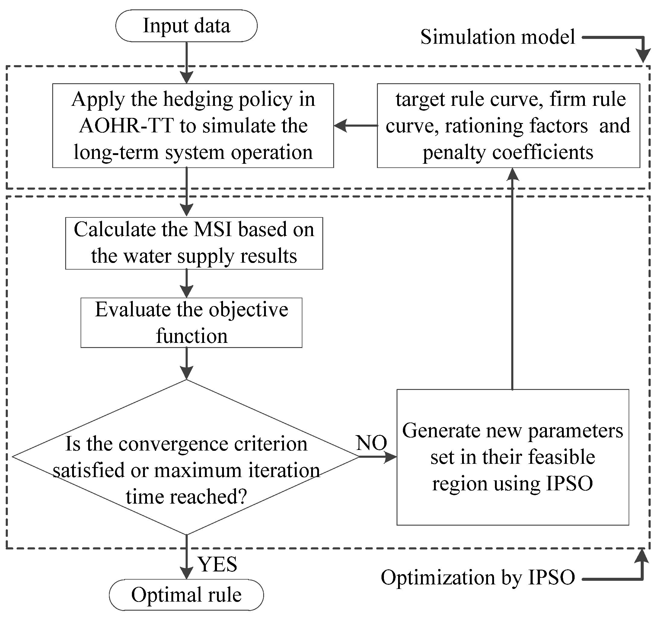
2.2. Formulation of the Optimization-Simulation Model for the AOHR-TT

The above derivation shows that the parameters in the AOHR-TT consist of the storage targets for each time interval (i.e., target rule curves ($T{R}_t$) and firm rule curves ($F{R}_t$)), rationing factors (${\alpha }_1$ and ${\alpha }_2$) and penalty coefficients ($P_i$, i = 1, 2, 3, 4, 5), which can be based on either optimization or expert knowledge. In this paper, an optimization-simulation model is used to determine these parameters. Optimization-simulation models combine optimization of the long-term operation benefits, which enables determination of the optimal parameter values, and the simulation of operation rules over particular time intervals, which allows the performance of the system to be measured for given parameter values [23].

2.2.1. Optimization Model

Optimization Objective

An effective index of water shortage is required to evaluate the effectiveness of the optimal hedging rules over long time periods. By modifying the shortage index (SI) of HEC [24,25], Hsu and Cheng [26] developed the modified shortage index (MSI), which considers the important characteristics of the uneven distribution of hydrologic conditions and the associated socioeconomic impacts. In this paper, the MSI is used to establish the optimization objective as follows:

$$L=\min \left\{\frac{100}{T}{\displaystyle \sum _{t=1}^T{(\frac{T{S}_t}{D_t})}^2}\right\}$$

(24)

where $T{S}_t$ is the total shortage in the tth period; $D_t$ is the demand target in the tth period; T is the total number of time periods; and L is the optimization objective for long-term periods.

System Constraints

The parameters of the AOHR-TT are taken as decision variables. The constraints for these decision variables are illustrated in Equation (25):

$$\{\begin{array}{l}0<F{R}_t\le T{R}_t\le K,t=1,2,\cdots 12\\ 1-MASR\le {\alpha }_2<{\alpha }_1<1\\ 0<P_1<P_2<P_3\\ 0<P_4<P_5\end{array}$$

(25)

where $MASR$ is the maximum allowed shortage ratio in a single period and is defined as the maximum value of the ratio between the current water deficits caused by rationing and the current demand target. $MASR$ is obtained based on the practical requirement for water supply.

Moreover, the water balance of the reservoir is considered a constraint (Equation (2)). In addition, the water-supply reliability must be equal to or more than the planned reliability. In this paper, the water-supply reliability is taken based on the statistics of a period and can be calculated using Equation (26):

$$Rel=\frac{T-{\displaystyle \sum _{t=1}^T{\sigma }_t}}{T}({\sigma }_t=\{\begin{array}{l}1R_t<D_t\\ 0otherwise\end{array}),t=1,2,\mathrm{...},T$$

(26)

where $Rel$ is the actual water-supply reliability and ${\displaystyle \sum _{t=1}^T{\sigma }_t}$ denotes the accumulated number of operational periods with rationing.

Method of Solution

In recent years, heuristic search algorithms combined with simulations have been widely used to solve complicated engineering problems characterized by nonlinearity, discontinuity, and discreteness. In this field, the particle swarm optimization (PSO) algorithm, originally proposed by Kennedy and Eberhart [27], is one of the most popular methods. As a population-based search algorithm, PSO is simple and efficient but exhibits premature convergence, especially in complex multi-peak search problems [28]. An improved particle swarm optimization (IPSO) algorithm was proposed by Jiang et al. [28] to improve this limitation of the standard PSO. IPSO has been verified to have greater breadth and depth when searching and has been widely applied in reservoir system operations [29,30]. In this paper, IPSO is adopted to solve the optimization model for the AOHR-TT for long-term operation. In IPSO, a population of particles is randomly sampled from the feasible space, and the population is then partitioned into several sub-swarms in which the particles evolve based on PSO. After a certain number of generations, the total population is shuffled, and particles are reassigned to sub-swarms to ensure the exchange of information [28]. The details of IPSO can be found in the work of Jiang et al. [28].

2.2.2. Simulation Model

The purpose of the simulation model is to recreate the long-term operation of a reservoir system used to supply water [31]. On the premise that the decision variables in the proposed rule are given by the optimization model, the procedures to simulate the long-term operation of a single reservoir are as follows:

(1)

According to the relationship between the initial storage level and the present level of the rule curves, the hedging sub-rule in the AOHR-TT is triggered first. Then, the current release is obtained based on the current water availability.

(2)

The ending reservoir storage level in the current period is then obtained by the water balance equation, and it is used to determine which hedging sub-rule is triggered in the next period. At the end of this step, the simulation procedure returns to step (1).

In this way, the simulation model iterates until the reservoir operation comes to an end, which then provides the optimization model with statistic indices, such as the MSI, corresponding to this set of decision variables. These results can then be used to calculate the value of the objective function for further iterative optimization. A schematic overview of the optimization-simulation model used in this paper is shown in Figure 6.

Figure 6. Framework of the optimization-simulation model used to determine the optimal rule.

Figure 6. Framework of the optimization-simulation model used to determine the optimal rule.

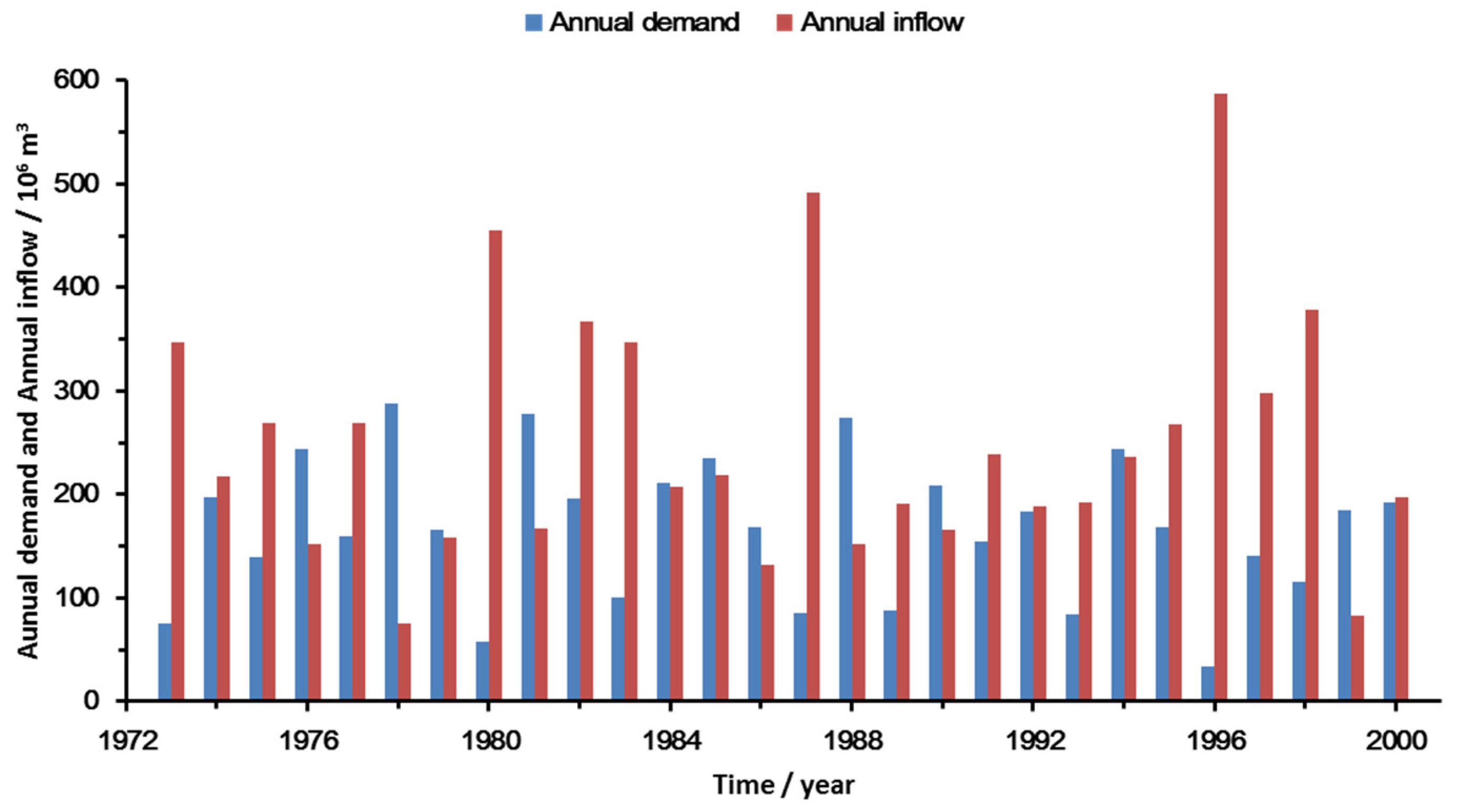
3. Study Area and Scenario Design

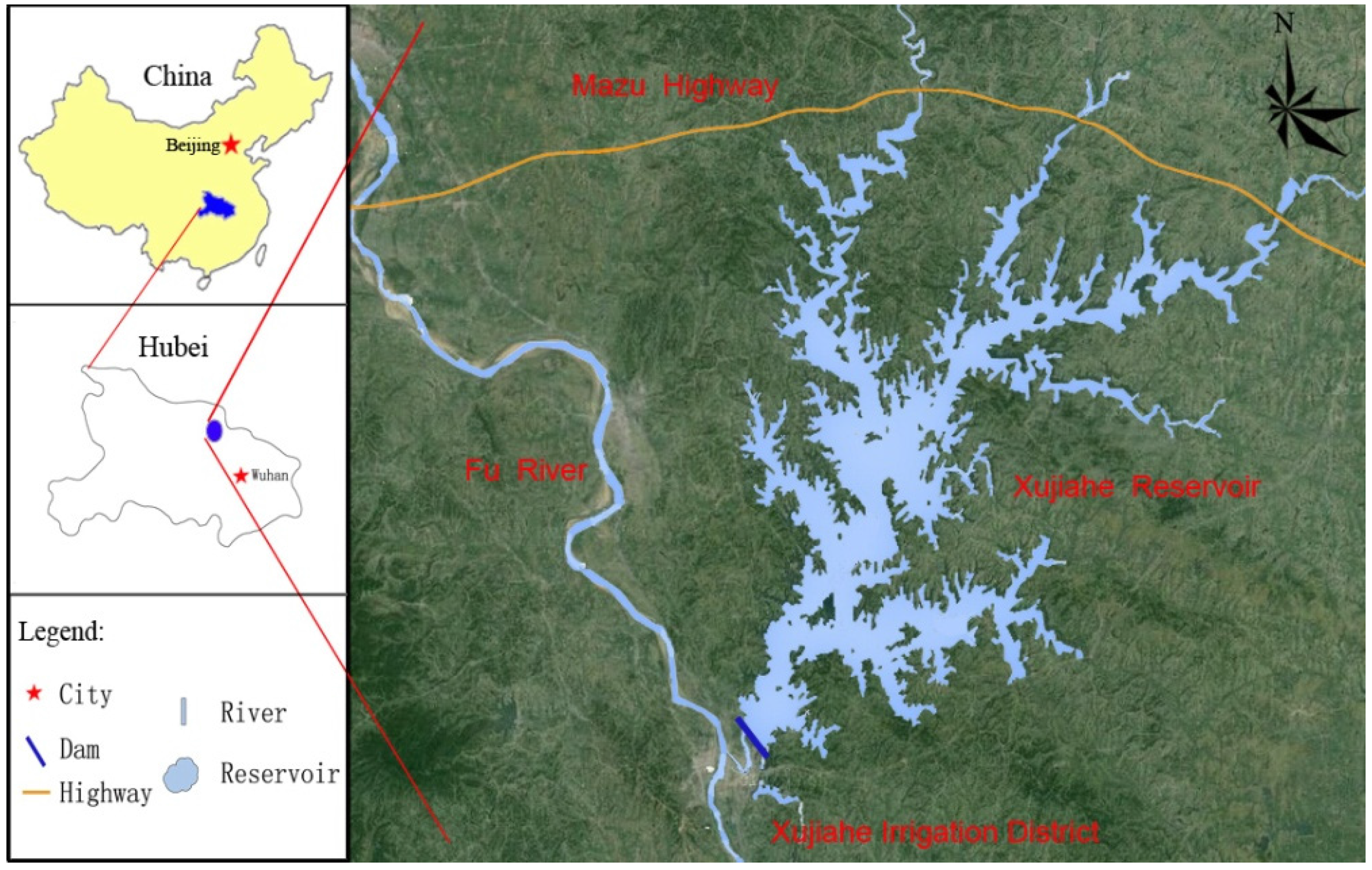
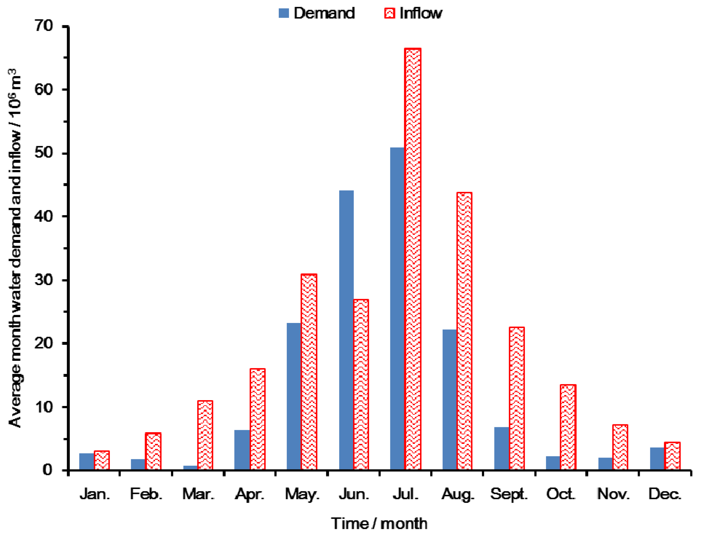
3.1. Study Area

The Xujiahe reservoir system was selected to test the proposed rule. The reservoir is located in Hubei province in central China (Figure 7), covers an area of 749 km², and receives an annual rainfall of approximately 1032 mm. The maximum active storage and dead storage of the Xujiahe reservoir are 2.99 × 10⁸ m³ and 1.41 × 10⁸ m³, respectively. The reservoir system is primarily designed to meet the water demands of agriculture in the irrigation district of Xujiahe.

Figure 7. The location of the Xujiahe reservoir.

Figure 7. The location of the Xujiahe reservoir.

The required inflow data for this reservoir comprise a 28-year series of hydrological records from 1973 to 2000. As shown in Figure 8, the monthly average inflow and the monthly average water demand of agriculture vary significantly throughout the year. Huge disparities between the annual inflows and the annual water demands of agriculture from 1973 to 2000 are present in Figure 9. The water losses resulting from evaporation and seepage were estimated based on the average water surface area in one operation period. In addition, the maximum allowed shortage ratio in a single period (MASR) is set to 0.2 based on the observed water demand of local agriculture, and the planned reliability is set to 0.8.

Figure 8. The monthly average inflow into Xujiahe reservoir and the monthly average water demand of agriculture.

Figure 8. The monthly average inflow into Xujiahe reservoir and the monthly average water demand of agriculture.

Figure 9. The annual demand and annual inflow into the system from 1973 to 2000.

Figure 9. The annual demand and annual inflow into the system from 1973 to 2000.

3.2. Scenario Design

In the proposed rule scenario, there are 31 decision variables in the optimization model, including two monthly rule curves (i.e., the target rule curve and the firm rule curve), two rationing factors for the agricultural demand, and five penalty coefficients for different reservoir zones and water shortage parts. The minimum and maximum penalty coefficients are set at 50 and 150, respectively, based on experience. The IPSO method includes three sub-swarms, each of which has 100 particles. The inertia weighting decreases linearly from 0.9 to 0.4 with increases in the iteration time, as recommended by Shi and Eberhart [32]. The acceleration constants are both 2.0, and the maximum number of iterations is 1000. For the sake of comparison and analysis, the exponent m of the loss functions in the AOHR-TT is set to 2.

To analyze the reasonableness and effectiveness of the proposed rule, five alternative scenarios, i.e., the SOP, conventional rule curves, the method proposed by Shiau [5] (referred to as Shiau’s method in this paper), Taghian’s method [20], and dynamic programming (DP), are used to generate and analyze the water supply results.

The SOP aims to release as much water as possible to meet the delivery target. The results of this model are used for comparison to those of the hedging rules in this paper.

The conventional rule curves (the target rule curve and the firm rule curve) divide the reservoir storage into three zones. The three zones of the initial reservoir storage level dictate the water supply and correspond to meeting the total demand or meeting some proportion (β₁ or β₂) of the demand (where 0 < β₂ < β₁ < 1). In this paper, Equation (24) is used as the optimization objective for long-term periods in the conventional rule curves scenario. The rationing factors (β₁ and β₂) and monthly rule curves are optimized as decision variables. As a discrete hedging rule, the operation results are compared with those of the continuous hedging rules.

Taghian’s method establishes zone-based hedging rules, as discussed in Section 2.1. Two operation objectives, i.e., operation goal for an individual time interval and optimization objective for long-term periods, are employed in this method. The former is defined as the minimization of the total cost in the system (linear objective function), which is solved via an LP algorithm, while the latter is expressed as the minimization of MSI (i.e., Equation (24), which is optimized via the genetic algorithms (GA). In this paper, IPSO is used in Taghian’s method instead of the GA for a fair comparison. Its decision variables are similar to those of the conventional rule curves. The difference between the two scenarios is that an LP optimization process for an individual time interval is applied in Taghian’s method that is not included in the conventional rule curves method. In this paper, Taghian’s method determines “benchmark” performance measurements for comparison to the results of the proposed rule.

Shiau’s method considers the balance between the release value and the carryover storage value in the two-period (time periods of t and t + 1) model to derive an analytical release rule in which the operation goal for an individual time interval is expressed as the weighted sum of the normalized deviation from the current release and carryover storage targets. Based on the predefined target rule curve, the shortage-related indices are calculated in this method via the two-period roll from the beginning of operation period to the end of long-term periods. This method can make the shortage-related indices improved for an individual time interval, but may perform poorly in the water-shortage cumulative effects over the long-term periods due to the negligence of the effect of the inflow in third period on the second period [8]. Therefore, in this paper, Shiau’s method is modified by coupling the optimization objective for long-term periods, i.e., Equation (24), to improve the shortage-related indices for a fair comparison. The monthly weighting factors (w_t) and monthly target rule curve, which have a significant impact on the operation benefits from long-term periods, are optimized as decision variables via IPSO. The results of Shiau’s method, a continuous hedging rule, are compared to those of the discrete hedging rule. This scenario and the proposed rule are both analytical continuous hedging rules. Thus, the results of this method can also be used for comparison to those of the proposed rule.

The DP model is one of the most popular optimization models for reservoir operation because of its ability to handle nonlinear, noncontinuous objective functions and constraints as well as temporally sequential reservoir decision making [33]. It can decompose a multi-stage reservoir operation problem into a series of two-stage problems via the recursive function in a backward form [33,34,35,36]. In this paper, Equation (24) is employed as the optimization objective for long-term periods in the DP model and it is solved via a discrete dynamic programming algorithm. Unlike the decision variables in the other scenarios, which are only monthly parameters on hedging throughout a year, the long-term releases are defined as decision variables in the DP model. Meanwhile, the inflow series for the entire control horizon are assumed to be known and implicitly used to make release decision in each period of DP while the current inflow is given in other scenarios. Therefore, the operation performance of the other scenarios is inferior to that of DP. However, the results from DP cannot be directly applied to provide guidelines for reservoir manager in real world, because the long-term inflows series cannot be perfectively forecasted [37]. The intention of this paper is to derive the optimal practical operation rule only based on the current inflow, and DP is thus more useful to be regarded as the gold standard against which any other scenarios can be compared [23].

3.3. Evaluation Criteria

To evaluate reservoir performance, the MSI, reliability, and maximum one-month shortage ratio (MSR) are employed to analyze the differences between the operation results yielded by the proposed rule and the other scenarios. The MSR is defined as the maximum value of the one-month shortage ratio during the operation period and can be expressed as

$$MSR=\max \left\{\frac{\left|\min \left\{R_t-D_t,0\right\}\right|}{D_t}\times 100\%\right\},t=1,2,\mathrm{...},T$$

(27)

In addition, the correlation coefficient (R²) and Nash-Sutcliffe coefficient (NSE) are employed to evaluate the similarities between DP and the other scenarios.

4. Results and Discussion

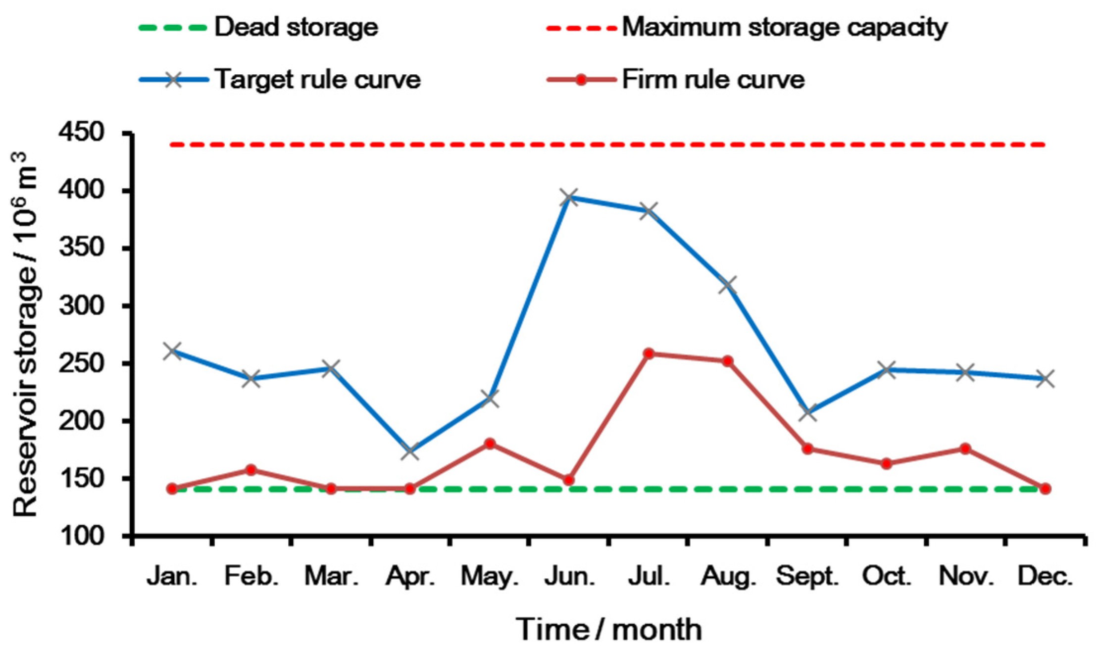
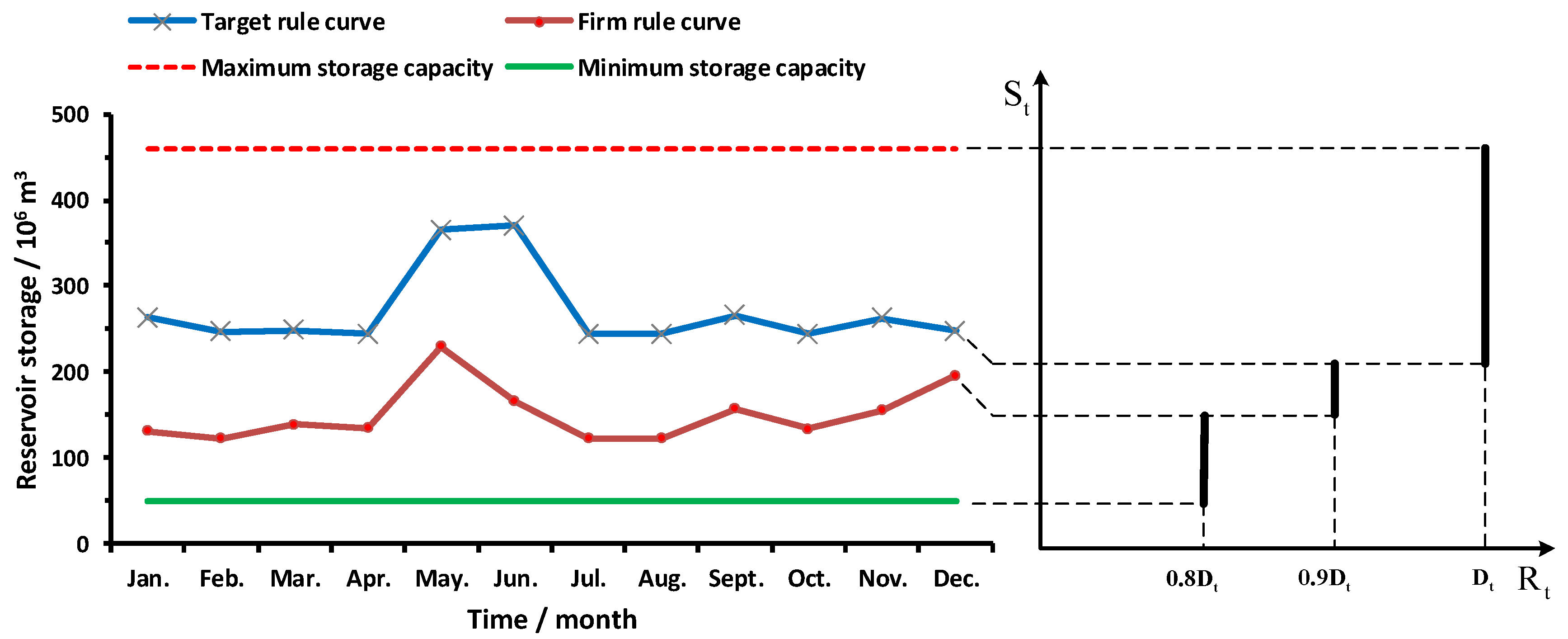
4.1. Analysis of Rule Curves in the Proposed Rule

The rule curves in the proposed rule obtained from the optimization-simulation model are shown in Figure 10. During the refill season between May and September, ample inflow leads to high rule curve values. In contrast, during the drawdown season, the rule curves are low due to a shortage of inflow. In particular, the lowest values of rule curves occur in April because more water is retained in advance in January. May is the beginning of the refill season. However, the level of the rule curves in May is low. This low value is due to the high water demand in May. Thus, as much water as possible is supplied, and the reservoir level is lowered to accommodate the massive impending inflow. In October, during drawdown season, the rule curves increase, which facilitates the storage of more water in advance of the demand during drawdown season.

Figure 10. The rule curves obtained according to the proposed rule.

Figure 10. The rule curves obtained according to the proposed rule.

The triggering frequencies of the hedging sub-rules for each month for 28 years (from 1973 to 2000) are presented in Figure 11. From the triggering mechanism perspective, the rule curves are used to trigger the hedging sub-rules. If the initial storage level at a time step rises above the rule curves, the hedging sub-rule with the least hedging is triggered. If the initial storage level is below the rule curves, the hedging sub-rule with the most hedging is triggered. For a month with low demand during the drawdown season, as shown in Figure 8, the amount of hedging in Rule 1 is sufficient. Thus, the levels of rule curves are kept low during the drawdown season, and Rule 1 is mostly triggered to guide the reservoir operation during the studied months of the 28 years. For a month with high demand during the refill season (Figure 8), Rule 2 or even Rule 3 will be triggered in order to increase hedging to reduce the risk of unacceptably large water deficits, as shown in Figure 11. Therefore, the rule curves in the months from June to August are kept high so that the frequency of significant hedging is higher. Invoking Rule 3 in May can alleviate the deficits in June so that the triggering frequency of Rule 3 in June is less than that in July. Therefore, the levels of the rule curves in May are higher than those of April.

Figure 11. The triggering frequencies of the three hedging sub-rules of the proposed rule for each month during the 28 years from 1973 to 2000.

Figure 11. The triggering frequencies of the three hedging sub-rules of the proposed rule for each month during the 28 years from 1973 to 2000.

4.2. Comparison and Analysis of Operation Scenarios

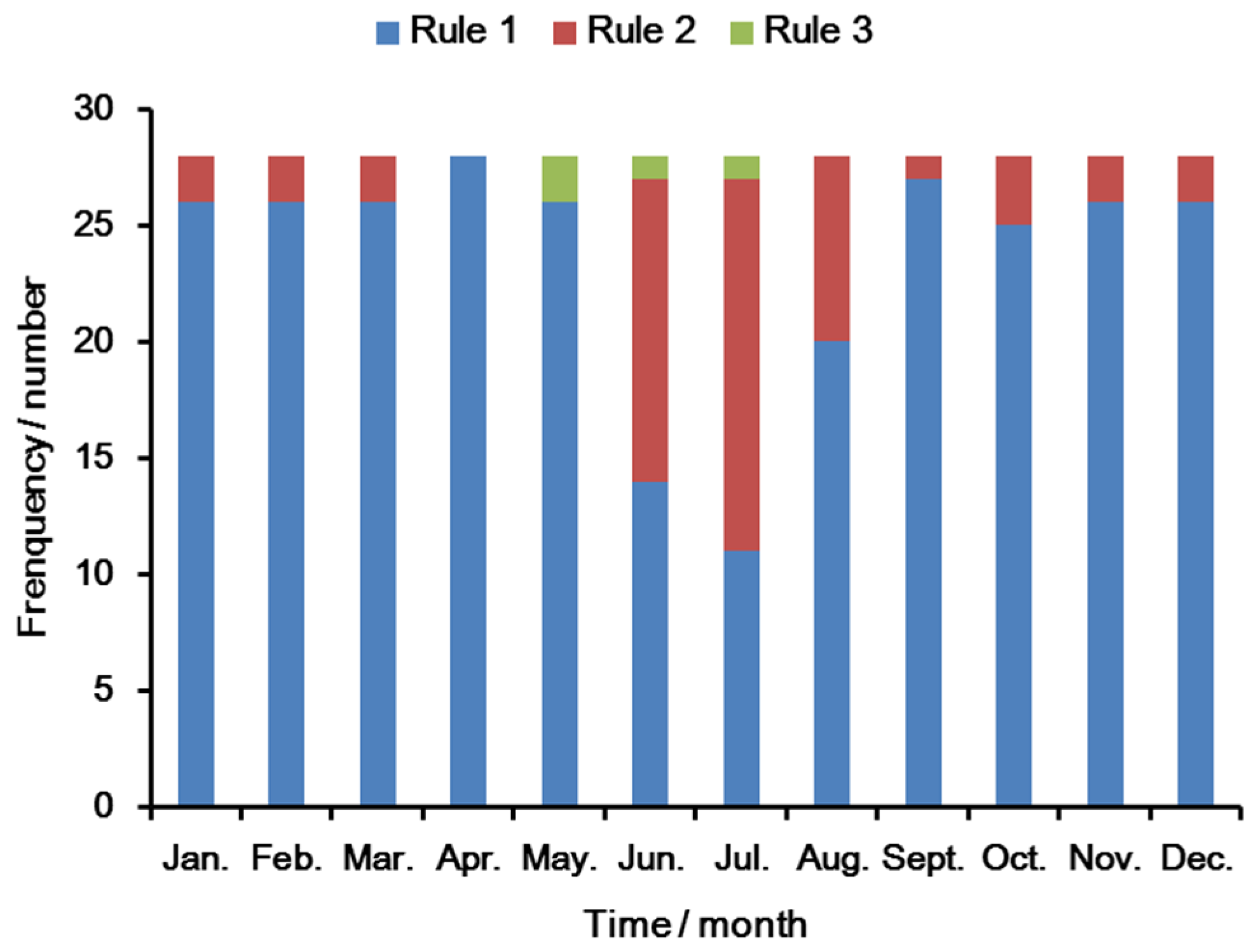
4.2.1. Comparison and Analysis of the Operation Types

The resulting parameters for the proposed rule, including the rationing factors (i.e., α₁ and α₂) and unit penalties (i.e., P₁, P₂, P₃, P₄ and P₅), are listed in Table 1. The proposed rule can be obtained by substituting the level of the rule curves and parameters into Equations (11)–(23). As an example, the optimal policy for a representative month (July) is illustrated in Figure 12. The operation policies obtained using Shiau’s method and the conventional rule curves for the representative month are shown in Figure 13 and Figure 14. Figure 12, Figure 13 and Figure 14 clearly show that three hedging sub-rules are applied in the operation of the reservoir under the proposed rule, whereas only one rule is applied in the operation of the reservoir under the other methods. The triggering mechanism for hedging in the proposed rule is based not only on the current water availability but also on the relationship between the initial storage level and the levels of the rule curves (target rule curve and firm rule curve). This relationship determines whether the amount of stored water is increased. When the initial storage level is less than the levels of the rule curves at the end of month (i.e., $T{R}_t$ and $F{R}_t$), more water is stored. When the initial storage level is greater than the levels of the rule curves, less water is stored. Therefore, unlike the case of Rule 1 shown in Figure 12, when water availability is within the range of $290\times {10}^6{m}^3\le W{A}_t\le 293\times {10}^6{m}^3$, Rule 2 prioritizes the storage of water until the target storage level ($T{R}_t$) is reached (i.e., $W{A}_t=291\times {10}^6{m}^3$). A similar difference exists between Rule 2 and Rule 3. In contrast to the proposed rule, hedging is implemented only based on the current water availability or initial storage in the operation policies obtained using Shiau’s method and the conventional rule curves. Figure 12, Figure 13 and Figure 14 also show that the conventional rule curves produce a discrete form of the water supply curve (Figure 14), which leads to fixed rationing factors (0.8 and 0.9), whereas the proposed rule (Figure 12) and Shiau’s method (Figure 13) produce continuous forms with variable rationing factors. The amount of hedging is determined by the fixed rationing factors in the conventional rule curves scenario, whereas the amount of hedging is decided by the analytical expression of the water supply in the proposed rule and Shiau’s method. For each time step in the proposed rule, the linear hedging within the range bounded by SWA and EWA produces a step-wise hedging, which is obviously different from Shiau’s method. For Rule 1 in the propose rule, a large proportion of the water demand ($0.973D_t$, i.e., $50\times {10}^6{m}^3$ in July) is met within the range of $SW{A}_{2t}<W{A}_t\le EW{A}_{2t}$, which leads to a lower marginal benefit of release in this range compared with that in the range of $SW{A}_{3t}<W{A}_t\le EW{A}_{3t}$. Therefore, the slope of the linear hedging (0.552) in the range of $SW{A}_{2t}<W{A}_t\le EW{A}_{2t}$ is smaller than that (0.680) in the range of $SW{A}_{3t}<W{A}_t\le EW{A}_{3t}$. The operational form obtained by Taghian’s method is not discussed because it is built on the basis of an LP model run for each time step.

Table 1. The parameters of the proposed rule.

Parameters
α1	α2	P1	P2	P3	P4	P5
0.973	0.838	50.0	67.9	144.9	55.1	68.1

Table 1. The parameters of the proposed rule.

Parameters
α1	α2	P1	P2	P3	P4	P5
0.973	0.838	50.0	67.9	144.9	55.1	68.1

Figure 12. The operation policy in July obtained using the proposed rule.

Figure 12. The operation policy in July obtained using the proposed rule.

Figure 13. The operation policy in July obtained using Shiau’s method.

Figure 13. The operation policy in July obtained using Shiau’s method.

Figure 14. The operation policy obtained using the conventional rule curves.

Figure 14. The operation policy obtained using the conventional rule curves.

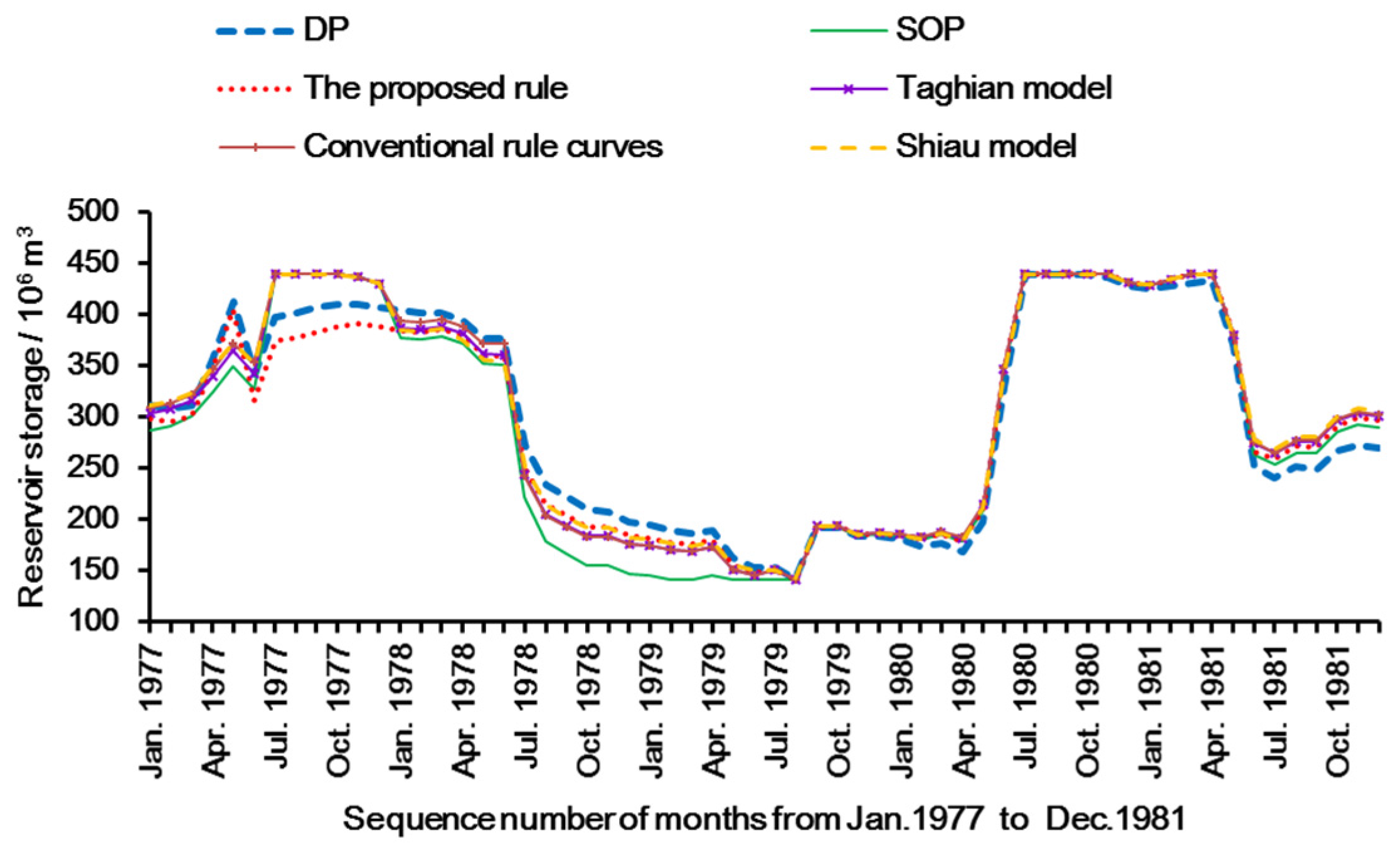
4.2.2. Comparison and Analysis of Long-Term Operation Results

The operation results of the different scenarios are shown in Table 2 and the probabilities of the rationing factors under different water supply scenarios are shown in Table 3. It can be seen from Table 2 that the highest MSI and MSR are obtained from the SOP, which indicates that its performance is the worst of all the scenarios. The SOP is intended to release amounts of water as close to the demand target as possible, which leads to the highest index of reliability (98.5%). However, because of this, it ignores the risk of unacceptably large water deficits in the future, consequently leading to the worst performance in terms of MSI (0.5340) and MSR (100%). Under the SOP, the required minimal water demand is not satisfied because the MSR (100%) exceeds the MASR (80%). Unlike the SOP, discrete rationing factors for water supply are applied to the conventional rule curves scenario; thus, more water is stored in the reservoir by allowing small deficits, which results in lower reliability (82.44%) than that of the SOP. In this way, unacceptable larger magnitude deficits can be avoided; thus, the MSR under the conventional rule curves scenario can satisfy the corresponding constraints, and the MSI of this scenario (0.2470) is superior to that (0.5340) of the SOP. Table 3 shows that the rationing factors (RF) of the conventional rule curves only include RF = 0.8, RF = 0.9 and RF = 1. This discrete operation strategy for water supply can result in underutilization of the regulation capacity of the reservoir; therefore, the MSI values are inferior to those of the scenarios other than SOP. The rationing factors for water supply in Taghian’s method are decided by considering the relationship between the reservoir storage levels (initial storage level and ending storage level) and the levels of the rule curves for each time step, which allows the storage level to remain as close as possible to the target rule curve or firm rule curve. The rationing factors in this scenario are not limited to discrete values, and a higher probability (98.51%) of rationing factors within the range of $0.9<RF\le 1$ is obtained, which leads to the improved utilization of the regulation capacity of the reservoir compared with the conventional rule curves scenario. Therefore, the MSI and reliability of Taghian’s method is superior to those of the conventional rule curves. Shiau’s method applies continuous rationing factors to the water supply operation, which leads to better indices than the discrete hedging rule in this paper, i.e., the conventional rule curves. In contrast to Taghian’s method, the current benefit function in Shiau’s method is nonlinear and can exhibit the characteristic of “hedging”. Therefore, the MSI and MSR of Shiau’s method are improved and decreased by 46% and 0.3%, respectively. As shown in Table 2, the MSI of the proposed rule are obviously superior to the scenarios other than DP, and the lowest MSR (16.22%) is obtained. Table 2 also shows that the results of the proposed rule are closest to those of the DP model, indicating that the proposed rule is optimal. This is due to the application of different hedging sub-rules established based on two triggers that balance the benefits of release and storage. Therefore, the lowest MSR is achieved while attempting to best satisfy the water demand, which leads to a high probability (97.62%) of rationing factors within the range of $0.9<RF\le 1$, as shown in Table 3.

Table 2. The operation results of different scenarios.

Indices	Scenarios
	SOP	Conventional Rule Curves	Shiau’s Method	Taghian’s Method	DP Model	Proposed Rule
MSI	0.5340	0.2470	0.0840	0.1563	0.0533	0.0695
MSR	100.00%	20.00%	19.94%	20.00%	19.68%	16.22%
Reliability	98.50%	82.44%	82.74%	87.20%	93.40%	81.85%

Table 2. The operation results of different scenarios.

Indices	Scenarios
	SOP	Conventional Rule Curves	Shiau’s Method	Taghian’s Method	DP Model	Proposed Rule
MSI	0.5340	0.2470	0.0840	0.1563	0.0533	0.0695
MSR	100.00%	20.00%	19.94%	20.00%	19.68%	16.22%
Reliability	98.50%	82.44%	82.74%	87.20%	93.40%	81.85%

Table 3. The probabilities of rationing factors under different water supply scenarios.

Scenarios	Rationing Factors (RF) of the Scenarios
	RF = 0.8	0.8 < RF < 0.9	RF = 0.9	0.9 < RF < 1	RF = 1
Conventional Rule Curves	2.38%	0	15.18%	0	82.44%
Shiau’s Method	0	2.68%	0	14.58%	82.74%
Taghian’s Method	1.49%	0	0	11.31%	87.20%
Proposed Rule	0	2.08%	0	15.77%	81.85%

Table 3. The probabilities of rationing factors under different water supply scenarios.

Scenarios	Rationing Factors (RF) of the Scenarios
	RF = 0.8	0.8 < RF < 0.9	RF = 0.9	0.9 < RF < 1	RF = 1
Conventional Rule Curves	2.38%	0	15.18%	0	82.44%
Shiau’s Method	0	2.68%	0	14.58%	82.74%
Taghian’s Method	1.49%	0	0	11.31%	87.20%
Proposed Rule	0	2.08%	0	15.77%	81.85%

4.2.3. Comparison and Analysis of Critical-Period Operation Results

An alternative can be chosen to evaluate the reasonableness and effectiveness of the policy under critical periods when the inflows are low or demands are high [38]. As shown in Figure 8, a significant difference exists between the annual inflows and the annual water demand for agriculture in the five years from 1977 to 1981. Therefore, in this paper, these years are chosen as critical periods. Among them, the years of 1978 and 1979 feature successive periods of severe droughts. Table 4 shows that the proposed policy exhibits a better reservoir performance in comparison to the other scenarios. To be more exact, during the five years from 1977 to 1981, the lowest MSI (0.2618) and MSR values (16.22%) are obtained from the proposed rule. Moreover, in the worst drought year, 1979, the proposed rule yields the best results for all the indicators of reservoir performance among the hedging policies, which indicates that the proposed policy can provide the most reliable water supply while minimizing the degree of water deficits in years of severe drought. It should be noted that the hedging rules usually alleviate future water deficits at the cost of reducing the reliability of fully satisfying current demands (Table 4).

Table 4. The operation results of different scenarios during the critical periods.

Years	Indices	Scenarios
		SOP	Conventional Rule Curves	Shiau’s Method	Taghian’s Method	Proposed Rule
1977	MSI	0.0000	0.1667	0.0014	0.1464	0.0125
	MSR	0.00%	10.00%	1.29%	9.37%	2.74%
	Reliability	100.00%	83.33%	91.67%	83.33%	83.33%
1978	MSI	0.0000	1.0833	0.4698	0.4393	0.4591
	MSR	0.00%	20.00%	19.94%	9.37%	16.04%
	Reliability	100%	41.67%	50.00%	50.00%	41.67%
1979	MSI	14.9586	2.1667	0.9523	1.8459	0.7874
	MSR	100.00%	20.00%	19.80%	20.00%	16.22%
	Reliability	58.33%	8.33%	8.33%	8.33%	16.67%
1980	MSI	0.0000	0.5833	0.0375	0.5530	0.0188
	MSR	0.00%	20.00%	6.20%	20.00%	2.74%
	Reliability	100.00%	66.67%	66.67%	66.67%	75.00%
1981	MSI	0.0000	0.0833	0.0431	0.0732	0.0313
	MSR	0.00%	10.00%	7.17%	9.37%	4.74%
	Reliability	100.00%	91.67%	75.00%	91.67%	75%
5 years	MSI	2.9917	0.8167	0.3008	0.6116	0.2618
	MSR	100.00%	20.00%	19.94%	20.00%	16.22%
	Reliability	91.67%	58.33%	58.33%	60.00%	58.33%

Table 4. The operation results of different scenarios during the critical periods.

Years	Indices	Scenarios
		SOP	Conventional Rule Curves	Shiau’s Method	Taghian’s Method	Proposed Rule
1977	MSI	0.0000	0.1667	0.0014	0.1464	0.0125
	MSR	0.00%	10.00%	1.29%	9.37%	2.74%
	Reliability	100.00%	83.33%	91.67%	83.33%	83.33%
1978	MSI	0.0000	1.0833	0.4698	0.4393	0.4591
	MSR	0.00%	20.00%	19.94%	9.37%	16.04%
	Reliability	100%	41.67%	50.00%	50.00%	41.67%
1979	MSI	14.9586	2.1667	0.9523	1.8459	0.7874
	MSR	100.00%	20.00%	19.80%	20.00%	16.22%
	Reliability	58.33%	8.33%	8.33%	8.33%	16.67%
1980	MSI	0.0000	0.5833	0.0375	0.5530	0.0188
	MSR	0.00%	20.00%	6.20%	20.00%	2.74%
	Reliability	100.00%	66.67%	66.67%	66.67%	75.00%
1981	MSI	0.0000	0.0833	0.0431	0.0732	0.0313
	MSR	0.00%	10.00%	7.17%	9.37%	4.74%
	Reliability	100.00%	91.67%	75.00%	91.67%	75%
5 years	MSI	2.9917	0.8167	0.3008	0.6116	0.2618
	MSR	100.00%	20.00%	19.94%	20.00%	16.22%
	Reliability	91.67%	58.33%	58.33%	60.00%	58.33%

The effectiveness of an operation rule can be evaluated based on the similarity between the storage process obtained using that rule and that of DP. The reservoir storage processes produced by DP and the other scenarios during the critical periods from 1977 to 1981 are shown in Figure 15, and their similarities are evaluated in Table 5. The largest R² and NSE values, produced by the proposed rule, indicate the greatest similarity to the DP model. Therefore, the reservoir storage process obtained using the proposed rule achieves a high level of agreement with the optimal reservoir storage process. Thus, the proposed rule in this paper is reasonable and effective during critical periods.

Figure 15. The end-of-month reservoir storage levels obtained using dynamic programming (DP) and the other scenarios during the critical periods from 1977 to 1981.

Figure 15. The end-of-month reservoir storage levels obtained using dynamic programming (DP) and the other scenarios during the critical periods from 1977 to 1981.

Table 5. The similarity comparison of storage process produced by dynamic programming (DP) and the other scenarios during the critical periods.

Evaluation Criteria	Scenarios
	SOP	Conventional Rule Curves	Shiau’s Method	Taghian’s Method	Proposed Rule
R2	0.974	0.985	0.987	0.984	0.990
NSE	0.917	0.960	0.967	0.959	0.982

Table 5. The similarity comparison of storage process produced by dynamic programming (DP) and the other scenarios during the critical periods.

Evaluation Criteria	Scenarios
	SOP	Conventional Rule Curves	Shiau’s Method	Taghian’s Method	Proposed Rule
R2	0.974	0.985	0.987	0.984	0.990
NSE	0.917	0.960	0.967	0.959	0.982

5. Conclusions

This article proposes an analytical optimal hedging rule to minimize the effects of droughts, in which a two-step approach for hedging based on two triggers is developed. For this purpose, three hedging sub-rules are defined for the operation of a single reservoir by establishing triggers based on the relationship between the beginning storage level and the levels of the rule curves. In each sub-rule, the start and end of hedging is based on the current water availability. To obtain the optimal rule curves for long-term reservoir operation, an improved particle swarm optimization (IPSO) algorithm with a rule-based simulation model is developed. A single reservoir in central China is employed as a case study to analyze the effects of the proposed operation rule.

The following conclusions can be drawn from the analysis of the results. First, based on the three hedging sub-rules with two triggers for rationing supply, the reservoir operation performance metrics, such as MSI and MSR values, during both long-term and critical periods are significantly improved relative to the performance metrics of the commonly used single rules based only on the initial storage or water availability. Second, the proposed rule with step-wise hedging can balance the reliability of the water supply and the magnitude of the deficits during droughts. Consequently, the proposed rule exhibits the highest water supply reliability and lowest MSR in the worst drought year. Third, the analytical form of the proposed operation rule, without the LP model running for each time step in Taghian’s method, is favorable for analyzing the effects of hedging and guiding the operation of reservoirs.

In conclusion, the proposed rule can provide reasonable and efficient guidelines for the operation of a single reservoir at the planning and management stages. However, the quality of the hedging policy in Taghian’s method requires further discussion in future work because the triggering mechanism of the proposed rule is based on that policy. In addition, the theoretical or analytical proof for the performance improvement of the proposed rule during long-term periods needs to be further investigated.

References

1. Cancelliere, A.; Ancarani, A.; Rossi, G. Susceptibility of Water Supply Reservoirs to Drought Conditions. J. Hydrol. Eng. 1998, 3, 140–148. [Google Scholar] [CrossRef]
2. Bayazit, M.; Ünal, N.E. Effects of Hedging on Reservoir Performance. Water Resour. Res. 1990, 26, 713–719. [Google Scholar] [CrossRef]
3. Bower, B.T.; Hufschmidt, M.M.; Reedy, W.W. Operating Procedures: Their Role in the Design of Water-Resource Systems by Simulation Analyses; Harvard University Press: Cambridge, MA, USA, 1962; pp. 443–458. [Google Scholar]
4. Draper, A.; Lund, J. Optimal Hedging and Carryover Storage Value. J. Water Resour. Plan. Manag. 2003, 130, 83–87. [Google Scholar] [CrossRef]
5. Shiau, J.-T. Analytical Optimal Hedging with Explicit Incorporation of Reservoir Release and Carryover Storage Targets. Water Resour. Res. 2011, 47, W01515. [Google Scholar] [CrossRef]
6. Srinivasan, K.; Philipose, M.C. Evaluation and Selection of Hedging Policies Using Stochastic Reservoir Simulation. Water Resour. Manag. 1996, 10, 163–188. [Google Scholar] [CrossRef]
7. Srinivasan, K.; Philipose, M.C. Effect of Hedging on over-Year Reservoir Performance. Water Resour. Manag. 1998, 12, 95–120. [Google Scholar] [CrossRef]
8. You, J.-Y.; Cai, X. Hedging Rule for Reservoir Operations: 1. A Theoretical Analysis. Water Resour. Res. 2008, 44, W01415. [Google Scholar] [CrossRef]
9. Shiau, J.T.; Lee, H.C. Derivation of Optimal Hedging Rules for a Water-Supply Reservoir through Compromise Programming. Water Resour. Manag. 2005, 19, 111–132. [Google Scholar] [CrossRef]
10. Zhao, J.; Cai, X.; Wang, Z. Optimality Conditions for a Two-Stage Reservoir Operation Problem. Water Resour. Res. 2011, 47, W08503. [Google Scholar] [CrossRef]
11. Revelle, C.; Joeres, E.; Kirby, W. The Linear Decision Rule in Reservoir Management and Design: 1, Development of the Stochastic Model. Water Resour. Res. 1969, 5, 767–777. [Google Scholar] [CrossRef]
12. Houck, M.H.; Cohon, J.L.; ReVelle, C.S. Linear Decision Rule in Reservoir Design and Management: 6. Incorporation of Economic Efficiency Benefits and Hydroelectric Energy Generation. Water Resour. Res. 1980, 16, 196–200. [Google Scholar] [CrossRef]
13. Neelakantan, T.R.; Pundarikanthan, N.V. Hedging Rule Optimisation for Water Supply Reservoirs System. Water Resour. Manag. 1999, 13, 409–426. [Google Scholar] [CrossRef]
14. Ilich, N.; Simonovic, S.P.; Amron, M. The Benefits of Computerized Real-Time River Basin Management in the Malahayu Reservoir System. Can. J. Civ. Eng. 2000, 27, 55–64. [Google Scholar] [CrossRef]
15. Neelakantan, T.; Pundarikanthan, N. Neural Network-Based Simulation-Optimization Model for Reservoir Operation. J. Water Resour. Plan. Manag. 2000, 126, 57–64. [Google Scholar] [CrossRef]
16. Tu, M.; Hsu, N.; Yeh, W. Optimization of Reservoir Management and Operation with Hedging Rules. J. Water Resour. Plan. Manag. 2003, 129, 86–97. [Google Scholar] [CrossRef]
17. Hashimoto, T.; Stedinger, J.R.; Loucks, D.P. Reliability, Resiliency, and Vulnerability Criteria for Water Resource System Performance Evaluation. Water Resour. Res. 1982, 18, 14–20. [Google Scholar] [CrossRef]
18. Shih, J.; ReVelle, C. Water-Supply Operations During Drought: Continuous Hedging Rule. J. Water Resour. Plan. Manag. 1994, 120, 613–629. [Google Scholar] [CrossRef]
19. Shih, J.-S.; ReVelle, C. Water Supply Operations During Drought: A Discrete Hedging Rule. Eur. J. Oper. Res. 1995, 82, 163–175. [Google Scholar] [CrossRef]
20. Taghian, M.; Rosbjerg, D.; Haghighi, A.; Madsen, H. Optimization of Conventional Rule Curves Coupled with Hedging Rules for Reservoir Operation. J. Water Resour. Plan. Manag. 2014, 140, 693–698. [Google Scholar] [CrossRef]
21. Zeng, X.; Hu, T.; Xiong, L.; Cao, Z.; Xu, C. Derivation of Operation Rules for Reservoirs in Parallel with Joint Water Demand. Water Resour. Res. 2015, 51, 9539–9563. [Google Scholar] [CrossRef]
22. Bazaraa, M.S.; Sherali, H.D.; Shetty, C.M. Nonlinear Programming: Theory and Algorithms; John Wiley & Sons: Hoboken, NJ, USA, 2013; pp. 188–199. [Google Scholar]
23. Koutsoyiannis, D.; Economou, A. Evaluation of the Parameterization-Simulation-Optimization Approach for the Control of Reservoir Systems. Water Resour. Res. 2003, 39, 1170. [Google Scholar] [CrossRef]
24. Hydraulic Engineering Center (US). Reservoir Yield, Generalized Computer Program 23-J2-L245; U.S. Army Corps of Engineers: Sacramento, CA, USA, 1966. [Google Scholar]
25. Hydraulic Engineering Center (US). Reservoir Yield. In Hydrologic Engineering Methods for Water Resources Development; U.S. Army Corps of Engineers: Davis, CA, USA, 1975. [Google Scholar]
26. Hsu, N.; Cheng, K. Network Flow Optimization Model for Basin-Scale Water Supply Planning. J. Water Resour. Plan. Manag. 2002, 128, 102–112. [Google Scholar] [CrossRef]
27. Kennedy, J.; Eberhart, R. Particle Swarm Optimization. In Proceedings of the IEEE International Conference on Neural Networks, Perth, WA, USA, 27 November–1 December 1995.
28. Jiang, Y.; Hu, T.; Huang, C.; Wu, X. An Improved Particle Swarm Optimization Algorithm. Appl. Math. Comput. 2007, 193, 231–239. [Google Scholar] [CrossRef]
29. Guo, X.; Hu, T.; Zhang, T.; Lv, Y. Bilevel Model for Multi-Reservoir Operating Policy in Inter-Basin Water Transfer-Supply Project. J. Hydrol. 2012, 424–425, 252–263. [Google Scholar] [CrossRef]
30. Zeng, X.; Hu, T.; Guo, X.; Li, X. Water Transfer Triggering Mechanism for Multi-Reservoir Operation in Inter-Basin Water Transfer-Supply Project. Water Resour. Manag. 2014, 28, 1293–1308. [Google Scholar] [CrossRef]
31. Guo, X.; Hu, T.; Zeng, X.; Li, X. Extension of Parametric Rule with the Hedging Rule for Managing Multireservoir System During Droughts. J. Water Resour. Plan. Manag. 2012, 139, 139–148. [Google Scholar] [CrossRef]
32. Shi, Y.; Eberhart, R. A Modified Particle Swarm Optimizer, IEEE World Congress on Computational Intelligence. In Proceedings of the 1998 IEEE International Conference on Evolutionary Computation, Anchorage, AK, USA, 4–9 May 1998.
33. Zhao, T.; Cai, X.; Lei, X.; Wang, H. Improved Dynamic Programming for Reservoir Operation Optimization with a Concave Objective Function. J. Water Resour. Plan. Manag. 2011, 138, 590–596. [Google Scholar] [CrossRef]
34. Loucks, D.P.; Stedinger, J.R.; Haith, D.A. Water Resource Systems Planning and Analysis; Prentice-Hall: Englewood Cliffs, NJ, USA, 1981. [Google Scholar]
35. Yeh, W.W.G. Reservoir Management and Operations Models: A State-of-the-Art Review. Water Resour. Res. 1985, 21, 1797–1818. [Google Scholar] [CrossRef]
36. Labadie, J. Optimal Operation of Multireservoir Systems: State-of-the-Art Review. J. Water Resour. Plan. Manag. 2004, 130, 93–111. [Google Scholar] [CrossRef]
37. Faber, B.A.; Stedinger, J.R. Reservoir Optimization Using Sampling SDP with Ensemble Streamflow Prediction (ESP) Forecasts. J. Hydrol. 2001, 249, 113–133. [Google Scholar] [CrossRef]
38. Oliveira, R.; Loucks, D.P. Operating Rules for Multireservoir Systems. Water Resour. Res. 1997, 33, 839–852. [Google Scholar] [CrossRef]