
Extent of Stream Burial and Relationships to Watershed Area, Topography, and Impervious Surface Area


Abstract
:1. Introduction
2. Materials and Methods
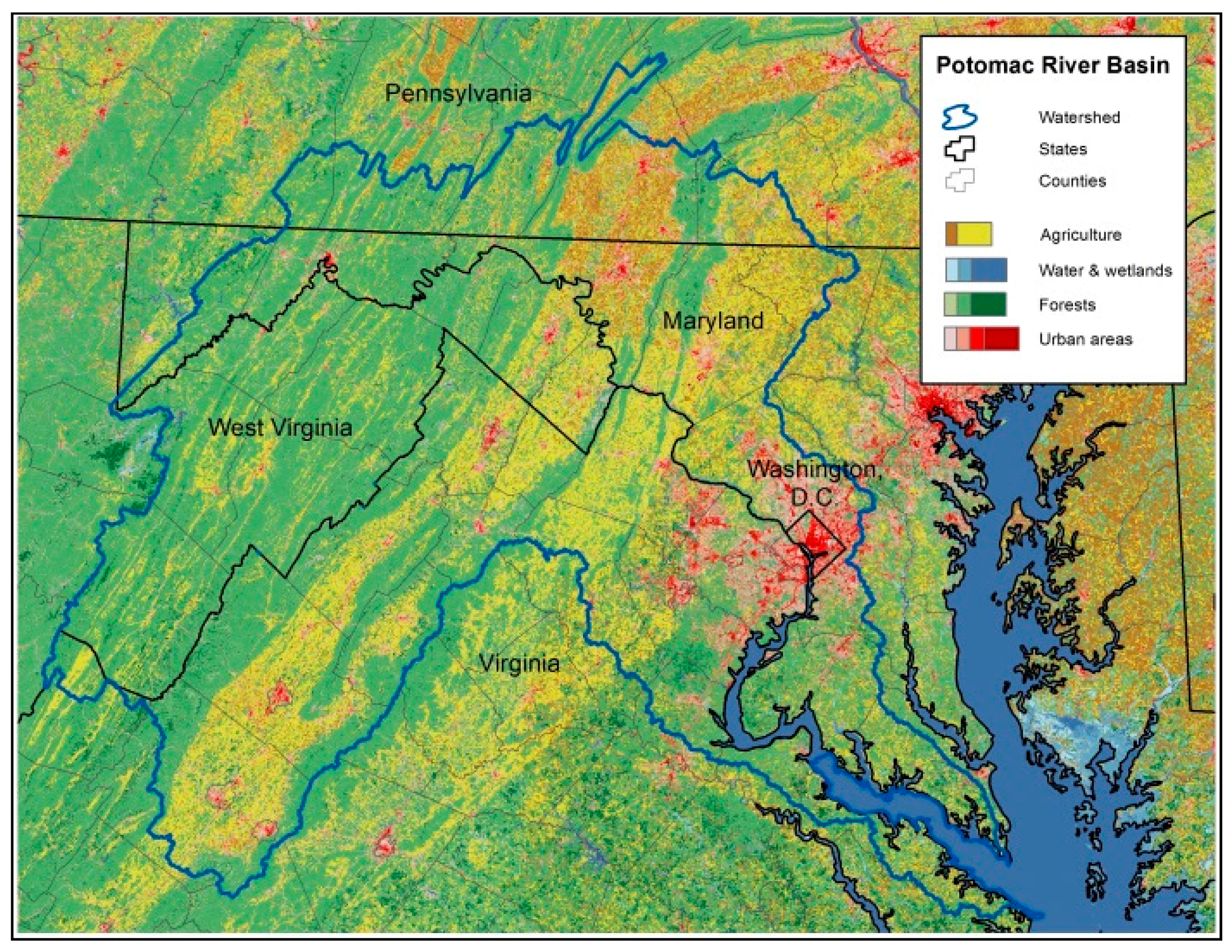
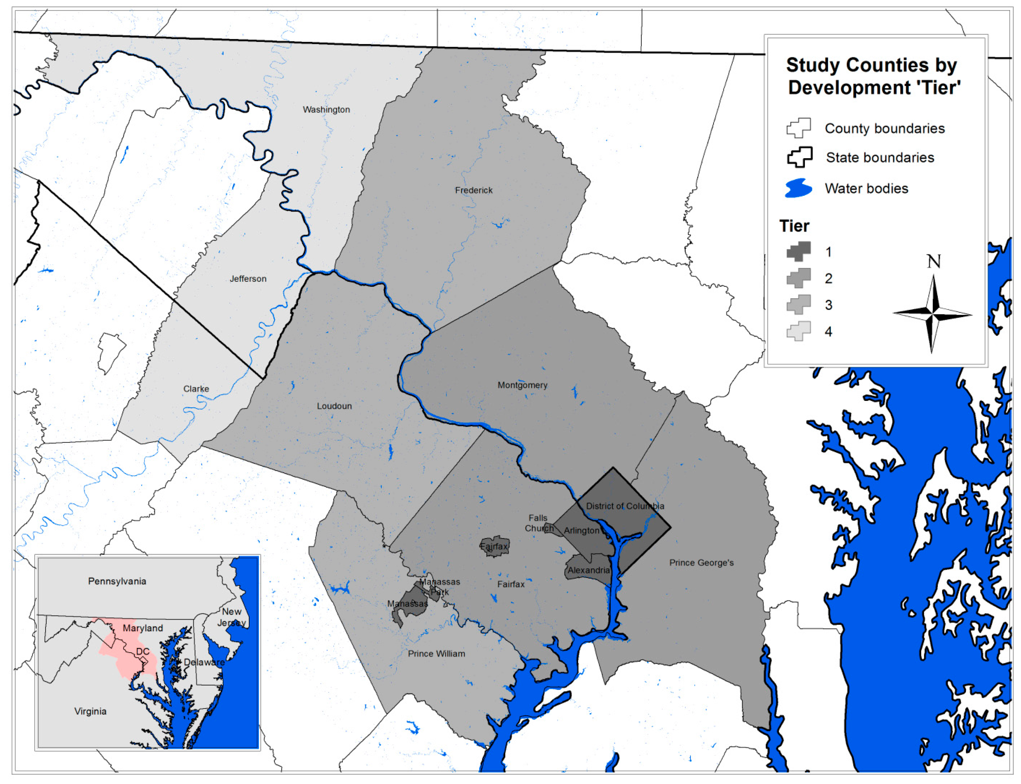
2.1. Study Area
2.2. Mapping Potential Stream Burial
2.3. Accuracy Analysis of Burial Classification
2.4. Analysis of Stream Burial Patterns across the PRB, in Relation to Slope and Catchment Area
3. Results
3.1. Burial Prediction Accuracy
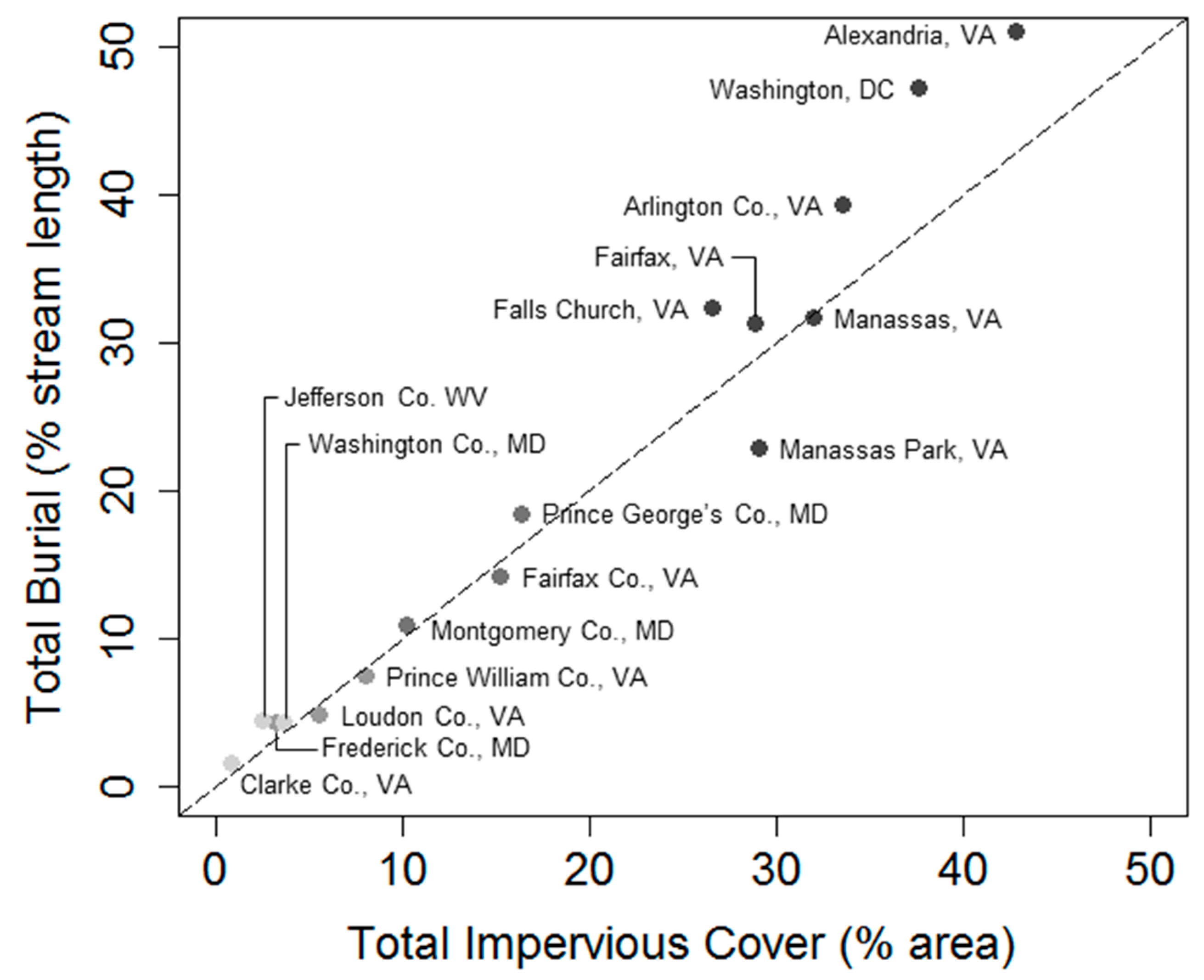
3.2. Relationship between Predicted Burial Rates and Impervious Cover
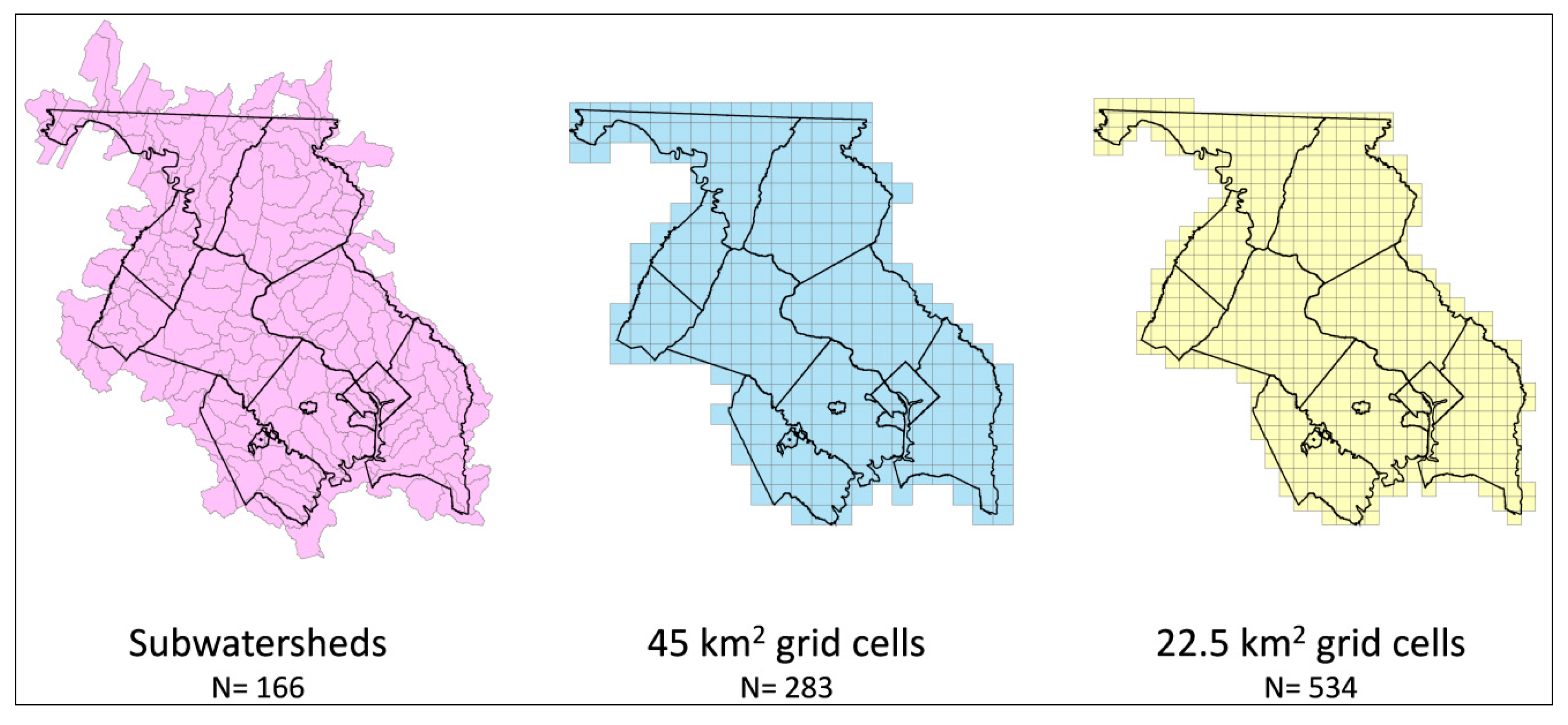
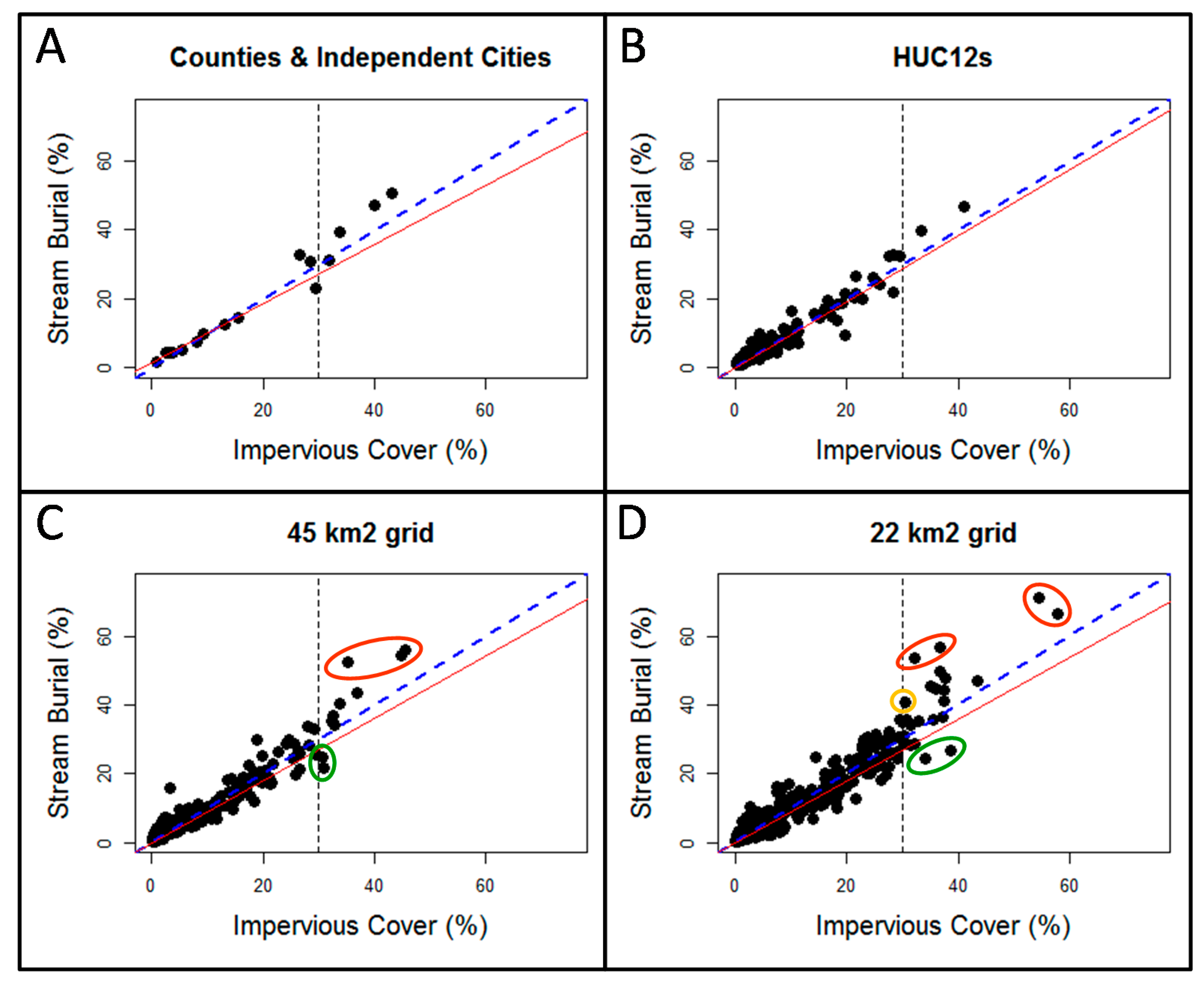
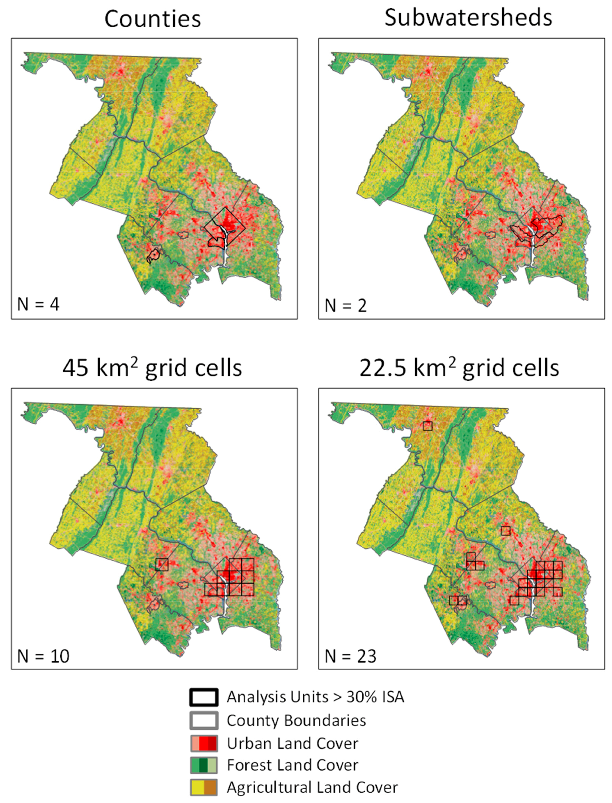
3.3. Effects of Scale on Burial/ISA Relationships
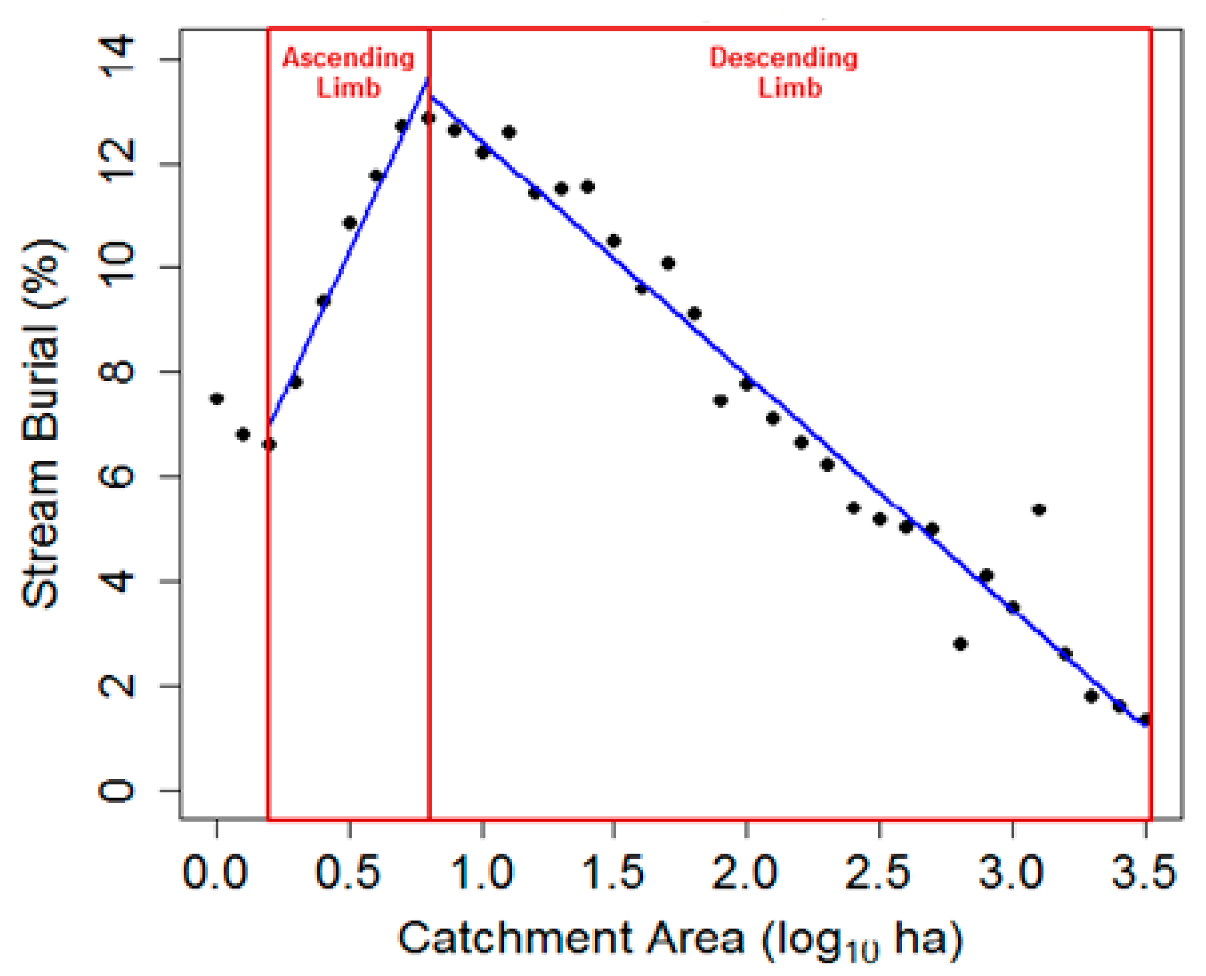
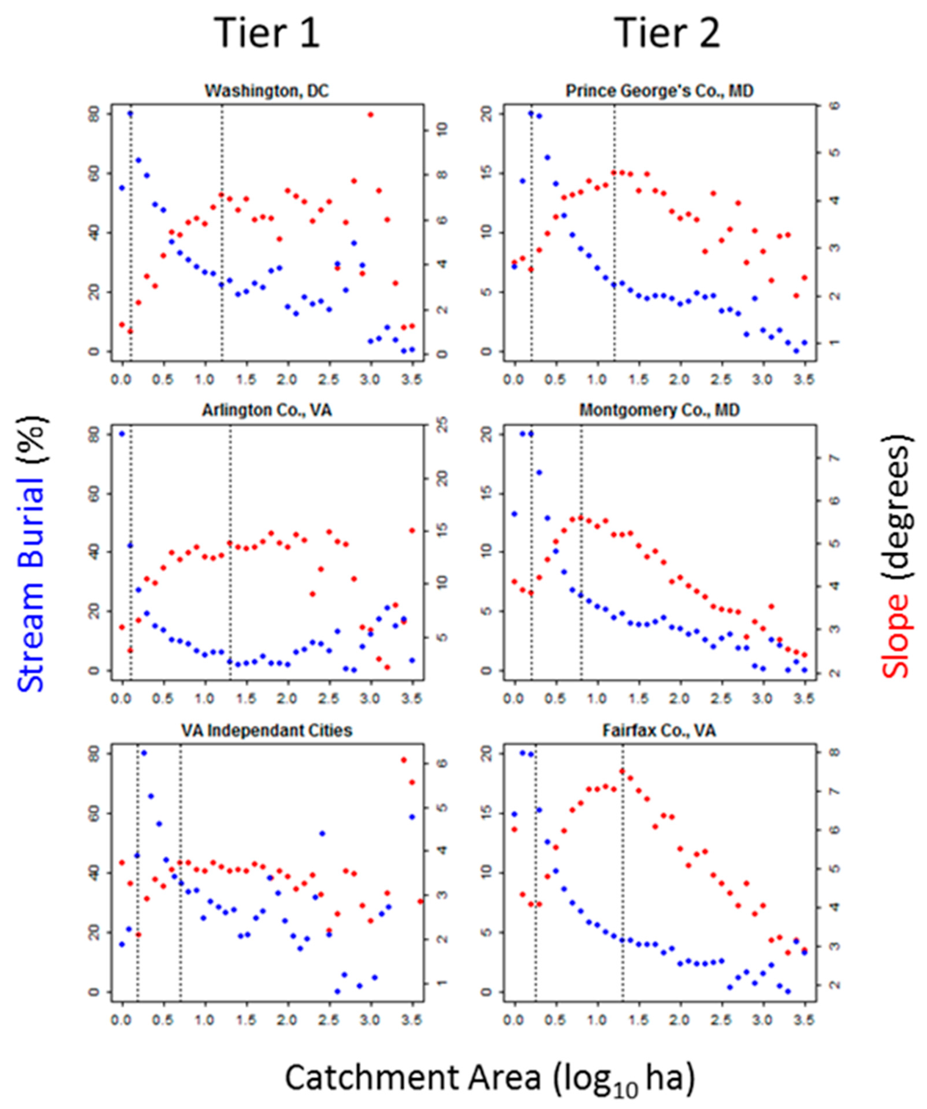
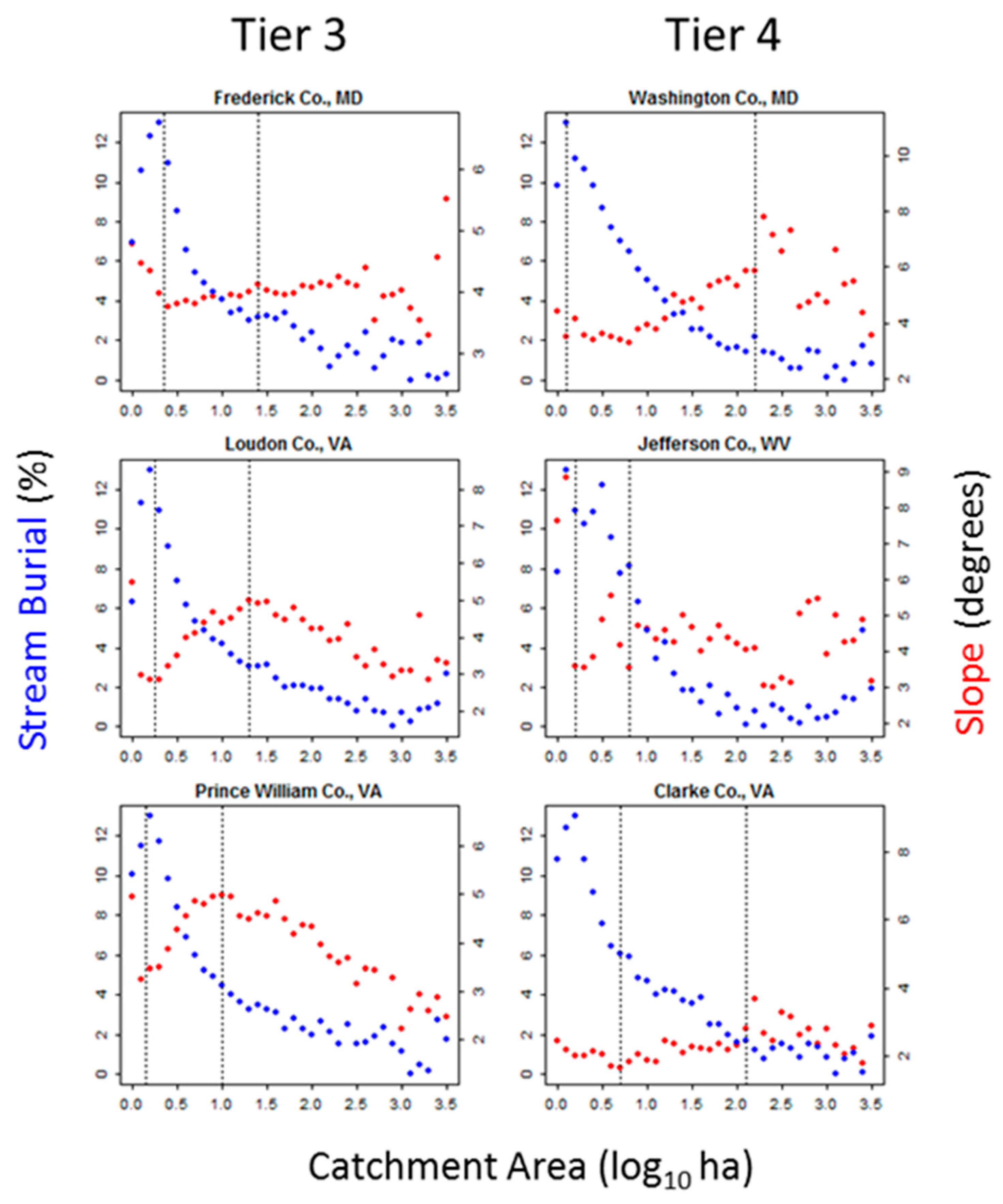
3.4. Relationship between Burial and Catchment Area
3.5. Relationship between Burial and Slope
4. Discussion
4.1. Relationship of Predicted Stream Burial to Impervious Surface Area (ISA) across Multiple Scales
4.2. Predicted Burial Patterns by Development Stage, and Relation to Catchment Area and Slope
4.3. Mapping Approach and Uncertainties
4.4. Future Work
5. Conclusions
Acknowledgments
Author Contributions
Conflicts of Interest
References
- Barton, N.J. The Lost Rivers of London: A Study of Their Effects upon London and Londoners, and the Effects of London and Londoners on Them; Historical Publications: London, UK, 1992; p. 168. [Google Scholar]
- Elmore, A.J.; Kaushal, S.S. Disappearing headwaters: Patterns of stream burial due to urbanization. Front. Ecol. Environ. 2008, 6, 308–312. [Google Scholar] [CrossRef]
- Roy, A.H.; Dybas, A.L.; Fritz, K.M.; Lubbers, H.R. Urbanization affects the extent and hydrologic permanence of headwater streams in a midwestern US metropolitan area. J. N. Am. Benthol. Soc. 2009, 28, 911–928. [Google Scholar] [CrossRef]
- Napieralski, J.A.; Carvalhaes, T. Urban stream deserts: Mapping a legacy of urbanization in the United States. Appl. Geogr. 2016, 67, 129–139. [Google Scholar] [CrossRef]
- Napieralski, J.A.; Welsh, E.S. A century of stream burial in Michigan (USA) cities. J. Maps 2016, 1–5. [Google Scholar] [CrossRef]
- Leibowitz, S.G.; Wigington, P.J.; Rains, M.C.; Downing, D.M. Non-navigable streams and adjacent wetlands: Addressing science needs following the Supreme Court’s Rapanos decision. Front. Ecol. Environ. 2008, 6, 364–371. [Google Scholar] [CrossRef]
- Walsh, C.J.; Roy, A.H.; Feminella, J.W.; Cottingham, P.D.; Groffman, P.M.; Morgan, R.P. The urban stream syndrome: Current knowledge and the search for a cure. J. N. Am. Benthol. Soc. 2005, 24, 706–723. [Google Scholar] [CrossRef]
- United Nations World Water Assessment Programme (WWAP). Water for Sustainable Urban Human Settlements; Briefing Note, United Nations Human Settlements Programme (UN-HABITAT); United Nations World Water Assessment Programme (WWAP): Perugia, Italy, 2010; pp. 1–8. [Google Scholar]
- Wenger, S.J.; Roy, A.H.; Jackson, C.R.; Bernhardt, E.S.; Carter, T.L.; Filoso, S.; Gibson, C.A.; Hession, W.C.; Kaushal, S.S.; Martí, E.; et al. Twenty-six key research questions in urban stream ecology: An assessment of the state of the science. J. N. Am. Benthol. Soc. 2009, 28, 1080–1098. [Google Scholar] [CrossRef]
- Napieralski, J.A.; Keeling, R.; Dzieken, M.; Kobberstad, K.; Kelly, A.; Rhodes, C. Urban stream deserts as a consequence of excess stream burial in urban watersheds. Ann. Assoc. Am. Geogr. 2015, 105, 649–664. [Google Scholar] [CrossRef]
- Steele, M.K.; Heffernan, J.B.; Bettez, N.; Cavender-Bares, J.; Groffman, P.M.; Grove, J.M.; Hall, S.; Hobbie, S.E.; Larson, K.; Morse, J.L.; et al. Convergent surface water distributions in U.S. cities. Ecosystems 2014, 17, 685–697. [Google Scholar] [CrossRef] [Green Version]
- Meyer, J.L.; Paul, M.J.; Taulbee, W.K. Stream ecosystem function in urbanizing landscapes. J. N. Am. Benthol. Soc. 2005, 24, 602–612. [Google Scholar] [CrossRef]
- Meyer, J.L.; Poole, G.C.; Jones, K.L. Buried alive: Potential consequences of burying headwater streams in drainage pipes. In Proceedings of the 2005 Georgia Water Resourcees Conference, Athens, GA, USA, 25–27 April 2005; Hatcher, K.J., Ed.; University of Georgia: Athens, GA, USA, 2005. [Google Scholar]
- Kaushal, S.S.; Belt, K.T. They urban watershed continuum: Evolving spatial and temporal dimensions. Urban Ecosyst. 2012, 15, 409–435. [Google Scholar] [CrossRef]
- Beaulieu, J.J.; Mayer, P.M.; Kaushal, S.S.; Pennino, M.J.; Arango, C.P.; Balz, D.A.; Canfield, T.J.; Elonen, C.M.; Fritz, K.M.; Hill, B.H.; et al. Effects of urban stream burial on organic matter dynamics and reach scale nitrate retention. Biogeochemistry 2014, 121, 107–126. [Google Scholar] [CrossRef]
- Hope, A.; McDowell, W.; Wollheim, W. Ecosystem metabolism and nutrient uptake in an urban, piped headwater stream. Biogeochemistry 2014, 121, 167–187. [Google Scholar] [CrossRef]
- Pennino, M.J.; Kaushal, S.S.; Bealieu, J.J.; Mayer, P.M.; Arango, C.P. Effects of urban stream burial on nitrogen uptake and ecosystem metabolism: Implications for watershed nitrogen and carbon fluxes. Biogeochemistry 2014, 121, 247–269. [Google Scholar] [CrossRef]
- Booth, D.B.; Jackson, C.R. Urbanization of aquatic systems: Degradation thresholds, stormwater detection, and the limits of mitigation. J. Am. Water Resour. Assoc. 1997, 33, 1077–1090. [Google Scholar] [CrossRef]
- Paul, M.J.; Meyer, J.L. Streams in the Urban Landscape. Annu. Rev. Ecol. Syst. 2001, 32, 333–365. [Google Scholar] [CrossRef]
- Allan, J.D. Landscapes and riverscapes: The Influence of Land Use on Stream Ecosystems. Annu. Rev. Ecol. Evol. Syst. 2004, 35, 257–284. [Google Scholar] [CrossRef]
- Schueler, T.R.; Fraley-McNeal, L.; Cappiella, K. Is Impervious Cover Still Important? Review of Recent Research. J. Hydrol. Eng. 2009, 14, 309–315. [Google Scholar]
- Theobald, D.M.; Goetz, S.J.; Norman, J.B.; Jantz, P. Watersheds at Risk to Increased Impervious Surface Cover in the Conterminous United States. J. Hydrol. Eng. 2009, 14, 362–368. [Google Scholar] [CrossRef]
- Booth, D.B.; Karr, J.R.; Schauman, S.; Konrad, C.P.; Morley, S.A.; Larson, M.G.; Burges, S.J. Reviving urban streams: Land use, hydrology, biology, and human behavior 1. J. Am. Water Resour. Assoc. 2004, 40, 1351–1364. [Google Scholar] [CrossRef]
- Cuffney, T.F.; Brightbill, R.A.; May, J.T.; Waite, I.R. Responses of benthic macroinvertebrates to environmental changes associated with urbanization in nine metropolitan areas. Ecol. Appl. 2010, 20, 1384–1401. [Google Scholar] [CrossRef] [PubMed]
- King, R.S.; Baker, M.E.; Whigham, D.F.; Weller, D.E.; Jordan, T.E.; Kazyak, P.F.; Hurd, M.K. Spatial considerations for linking watershed land cover to ecological indicators in streams. Ecol. Appl. 2005, 15, 137–153. [Google Scholar] [CrossRef]
- Moore, A.A.; Palmer, M.A. Invertebrate biodiversity in agricultural and urban headwater streams: Implications for conservation and management. Ecol. Appl. 2005, 15, 1169–1177. [Google Scholar] [CrossRef]
- Wang, L.; Lyons, J.; Kanehl, P.; Bannerman, R. Impacts of Urbanization on Stream Habitat and Fish Across Multiple Spatial Scales. Environ. Manag. 2001, 28, 255–266. [Google Scholar] [CrossRef]
- Schiff, R.; Benoit, G. Effects of Impervious Cover at Multiple Spatial Scales on Coastal Watershed Streams. J. Am. Water Resour. Assoc. 2007, 43, 712–730. [Google Scholar] [CrossRef]
- Roy, A.H.; Shuster, W.D. Assessing Impervious Surface Connectivity and Applications for Watershed Management. J. Am. Water Resour. Assoc. 2009, 45, 198–209. [Google Scholar] [CrossRef]
- Claggett, P.R.; Jantz, C.A.; Goetz, S.J.; Bisland, C. Assessing Development Pressure in the Chesapeake Bay Watershed: An Evaluation of Two Land-Use Change Models. Environ. Monit. Assess. 2004, 94, 129–146. [Google Scholar] [CrossRef] [PubMed]
- Jantz, C.A.; Goetz, S.J. Analysis of scale dependencies in an urban land-use-change model. Int. J. Geogr. Inf. Sci. 2005, 19, 217–241. [Google Scholar] [CrossRef]
- Jenerette, G.D.; Wu, J. Analysis and simulation of land-use change in the central Arizona-Phoenix region, USA. Landsc. Ecol. 2001, 16, 611–626. [Google Scholar] [CrossRef]
- Kaushal, S.S.; McDowell, W.H.; Wollheim, W.M. Tracking evolution of urban biogeochemical cycles; Past, present, and future. Biogeochemistry 2014, 121, 1–21. [Google Scholar] [CrossRef]
- Kaushal, S.S.; McDowell, W.H.; Wollheim, W.M.; Johnson, T.A.N.; Mayer, P.M.; Belt, K.T.; Pennino, M.J. Urban evolution: The role of water. Water 2015, 7, 4063–4087. [Google Scholar] [CrossRef]
- Elmore, A.; Julian, J.; Guinn, S.; Fitzpatrick, M. Potential Stream Density in Mid-Atlantic US Watersheds. PLoS ONE 2013, 8, e74189. [Google Scholar] [CrossRef] [PubMed]
- Fry, J.; Xian, G.; Jin, S.; Dewitz, J.; Homer, C.; Yang, L.; Barnes, C.; Herold, N.; Wickham, J. Completion of the 2006 National Land Cover Database for the Conterminous United States. Photogramm. Eng. Remote Sens. 2011, 77, 859–864. [Google Scholar]
- Hothorn, T.; Hornik, K.; Zeileis, A. Unbiased recursive partitioning: A conditional inference framework. J. Comput. Graph. Stat. 2006, 15, 651–674. [Google Scholar] [CrossRef]
- Lookingbill, T.R.; Kaushal, S.S.; Elmore, A.J.; Gardner, R.; Eshleman, K.N.; Hilderbrand, R.H.; Morgan, R.P.; Boynton, W.R.; Palmer, M.A.; Dennison, W.C. Altered ecological flows blur boundaries in urbanizing watersheds. Ecol. Soc. 2009, 14, 10. [Google Scholar]
- United States Census Bureau. United States Census 2000; U.S. Department of Commerce: Washington, DC, USA, 2000.
- R Core Development Team. R: A Language and Environment for Statistical Computing; Version 3.0.1; R Foundation for Statistical Computing: Vienna, Austria, 2013. [Google Scholar]
- Environmental Systems Research Institute (ESRI). ArcGIS Desktop: Release 10.1; ESRI: Redlands, CA, USA, 2012. [Google Scholar]
- Morrill, R. Classic map revisited: The growth of megalopolis. Prof. Geogr. 2006, 58, 155–160. [Google Scholar] [CrossRef]
- Gesch, D.; Oimoen, M.; Greenlee, S.; Nelson, C.; Steuck, M.; Tyler, D. The National Elevation Dataset. Photogramm. Eng. Remote Sens. 2002, 68, 5–32. [Google Scholar]
- Tarboton, D.; Schreuders, K.; Watson, D.; Baker, M.; Anderssen, R.; Braddock, R.; Newham, L. Generalized terrain-based flow analysis of digital elevation models. In Proceedings of the 18th World Imacs Congress and Modsim09 International Congress on Modelling and Simulation, Cairns, Australia, 13–17 July 2009; pp. 2000–2006.
- Pickett, S.T. Space-for-time substitution as an alternative to long-term studies. In Long-Term Studies in Ecology; Springer: New York, NY, USA, 1989; pp. 110–135. [Google Scholar]
- Valiela, I.; Foreman, K.; Lamontagne, M.; Hersh, D.; Costa, J.; Peckol, P.; Demeoandreson, B.; Davanzo, C.; Babione, M.; Sham, C.; et al. Couplings of watersheds and coastal waters—Sources and consequences of nutrient enrichment in Waquoit Bay, Massachusetts. Estuaries 1992, 15, 443–457. [Google Scholar] [CrossRef]
- Grimm, N.; Grove, J.; Pickett, S.; Redman, C. Integrated approaches to long-term studies of urban ecological systems. Bioscience 2000, 50, 571–584. [Google Scholar] [CrossRef]
- Brown, L.R.; Cuffney, T.F.; Coles, J.F.; Fitzpatrick, F.; McMahon, G.; Steuer, J.; Bell, A.H.; May, J.T. Urban streams across the USA: Lessons learned from studies in 9 metropolitan areas. J. N. Am. Benthol. Soc. 2009, 28, 1051–1069. [Google Scholar] [CrossRef]
- Stranko, S.; Hilderbrand, R.; Palmer, M. Comparing the Fish and Benthic Macroinvertebrate Diversity of Restored Urban Streams to Reference Streams. Restor. Ecol. 2012, 20, 747–755. [Google Scholar] [CrossRef]
- Diaz-Porras, D.; Gaston, K.; Evans, K. 110 Years of change in urban tree stocks and associated carbon storage. Ecol. Evol. 2014, 4, 1413–1422. [Google Scholar] [CrossRef] [PubMed]
- Netzband, M.; Stefanov, W.L.; Redman, C.L. Applied Remote Sensing for Urban. Planning, Governance and Sustainability; Springer: Berlin, Germany, 2007. [Google Scholar]
- Stammler, K.; Yates, A.; Bailey, R. Buried streams: Uncovering a potential threat to aquatic ecosystems. Landsc. Urban. Plan. 2013, 114, 37–41. [Google Scholar] [CrossRef]
- Freeman, M.C.; Pringle, C.M.; Jackson, C.R. Hydrologic Connectivity and the Contribution of Stream Headwaters to Ecological Integrity at Regional Scales 1. J. Am. Water Resour. Assoc. 2007, 43, 5–14. [Google Scholar] [CrossRef]


| Counties and Independent Cities | Area (km2) | Potential Stream Length (km) | Impervious Cover (%) | Stream Burial (%) | |
|---|---|---|---|---|---|
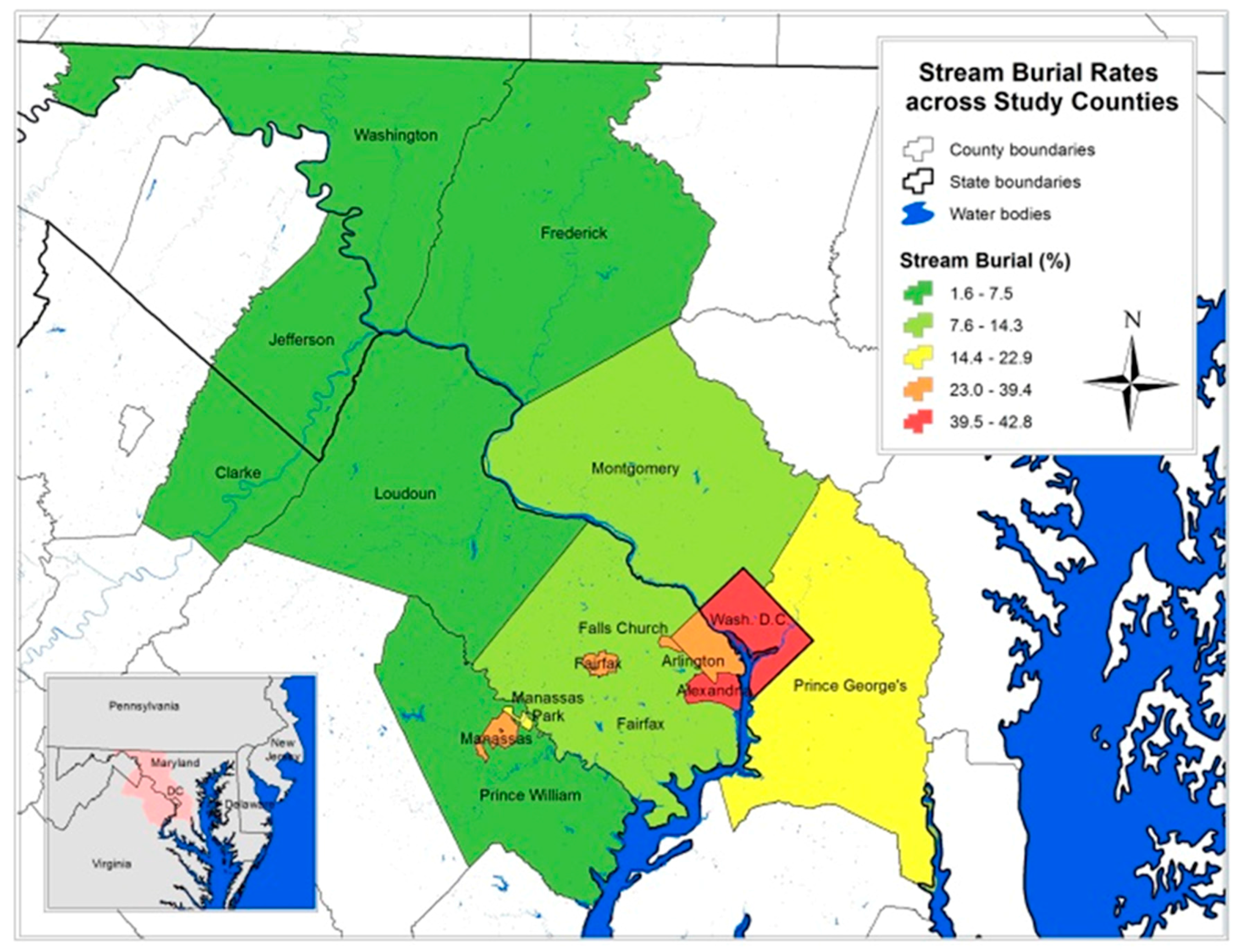
| Tier 1 | Washington, DC | 177.0 | 325.8 | 37.6 | 47.3 |
| Arlington County, VA | 67.3 | 170.9 | 33.6 | 39.4 | |
| City of Alexandria, VA | 39.9 | 95.7 | 42.8 | 51.1 | |
| City of Fairfax, VA | 16.3 | 40.9 | 28.9 | 31.3 | |
| City of Falls Church, VA | 5.1 | 11.2 | 26.6 | 32.4 | |
| City of Manassas, VA | 25.8 | 49.1 | 32.0 | 31.7 | |
| City of Manassas Park, VA | 6.5 | 16.4 | 29.1 | 22.9 | |
| Tier 2 | Prince George’s County, MD | 1291.0 | 2984.5 | 16.4 | 18.5 |
| Montgomery County, MD | 1313.5 | 3830.8 | 10.2 | 11.0 | |
| Fairfax County, VA | 461.5 | 2803.9 | 15.2 | 14.3 | |
| Tier 3 | Frederick County, MD | 1728.4 | 4146.2 | 3.3 | 4.4 |
| Loudon County, VA | 1053.1 | 3555.3 | 5.5 | 4.9 | |
| Prince William County, VA | 902.3 | 2566.7 | 8.0 | 7.5 | |
| Tier 4 | Washington County, MD | 1210.9 | 2151.0 | 3.7 | 4.4 |
| Jefferson County, WV | 548.0 | 733.0 | 2.5 | 4.5 | |
| Clarke County, VA | 1349.6 | 658.4 | 0.9 | 1.6 |
| Model | Accuracy (%) | ||
|---|---|---|---|
| Intact | Buried | Overall | |
| Iterative | 92.7 | 55.8 | 83.1 |
| Full | 88.0 | 71.0 | 83.0 |
| Analysis Units | N | Mean Area (Range) | Area with >30% ISA |
|---|---|---|---|
| Counties and Independent Cities | 16 | 632.1 km2 (5.19–1728.50) | 292.01 km2 |
| Subwatersheds | 166 | 89.9 km2 (33.75–170.44) | 221.48 km2 |
| 45 km2 grid cells | 283 | 45 km2 | 450.24 km2 |
| 22.5 km2 grid cells | 534 | 22.5 km2 | 517.41 km2 |
| Counties | Max Burial % (FAC) | Local Minimum (FAC) | Local Maximum (FAC) | Ascending Slope | Ascending Intercept | Descending Slope | Descending Intercept | |
|---|---|---|---|---|---|---|---|---|
| Tier 1 | Washington, DC | 79.4 (3.0) | 0.1 | 1.2 | 37.20 | 10.10 | −9.28 | 65.21 |
| Arlington County, VA | 47.4 (3.5) | 0.1 | 1.3 | 21.75 | 18.34 | −13.30 | 65.60 | |
| Independent Cities, VA | 78.0 (3.4) | 0.2 | 0.8 | 36.09 | 17.82 | 2.48 † | 34.96 † | |
| Tier 2 | Prince George’s County, MD | 15.0 (1.3) | 0.2 | 1.2 | 7.36 | 6.90 | −3.71 | 19.59 |
| Montgomery County, MD | 12.9 (0.8) | 0.2 | 0.8 | 11.06 | 4.75 | −4.48 | 16.88 | |
| Fairfax County, VA | 18.6 (1.3) | 0.25 | 1.3 | 9.95 | 6.64 | −6.93 | 26.89 | |
| Tier 3 | Frederick County, MD | 9.1 (3.5) | 0.35 | 1.4 | 0.89 | 3.35 | 0.22 † | 4.10 † |
| Loudon County, VA | 7.3 (0.0) | 0.25 | 1.3 | 3.61 | 1.88 | −1.62 | 8.30 | |
| Prince William County, VA | 9.0 (1.0) | 0.15 | 1.0 | 5.25 | 4.34 | −2.63 | 11.83 | |
| Tier 4 | Washington County, MD | 8.2 (2.3) | 0.1 | 2.2 | 1.74 | 1.42 | −2.90 | 13.46 |
| Jefferson County, WV | 12.6 (0.1) | 0.2 | 0.8 | 1.78 † | 3.19 † | −0.08 † | 4.45 † | |
| Clarke County, VA | 3.8 (2.2) | 0.7 | 2.1 | 0.85 | −0.01 | −1.12 † | 5.16 † | |
| Counties | Limb | FAC | R2 | SST | SLOPE | R2 | SST | |
|---|---|---|---|---|---|---|---|---|
| Tier 1 | Washington, DC | Ascending | *** | 0.91 | 2183.87 | *** | 0.95 | 2183.9 |
| Descending | * | 0.18 | 5624.6 | --- | - | - | ||
| Arlington County, VA | Ascending | *** | 0.65 | 1335.17 | *** | 0.96 | 1335.17 | |
| Descending | ** | 0.38 | 4672.4 | *** | 0.62 | 4672.4 | ||
| Independent Cities, VA | Ascending | ** | 0.81 | 450.05 | --- | - | - | |
| Descending | --- | - | - | --- | - | - | ||
| Tier 2 | Prince George’s County, MD | Ascending | *** | 0.86 | 69.312 | *** | 0.95 | 69.313 |
| Descending | *** | 0.75 | 210.571 | *** | 0.71 | 210.57 | ||
| Montgomery County, MD | Ascending | *** | 0.96 | 35.493 | *** | 0.99 | 35.492 | |
| Descending | *** | 0.97 | 379.15 | *** | 0.87 | 379.16 | ||
| Fairfax County, VA | Ascending | *** | 0.86 | 126.375 | *** | 0.99 | 126.374 | |
| Descending | *** | 0.96 | 503.26 | ** | 0.45 | 503.27 | ||
| Tier 3 | Frederick County, MD | Ascending | *** | 0.86 | 1.01895 | --- | - | - |
| Descending | --- | - | - | --- | - | - | ||
| Loudon County, VA | Ascending | *** | 0.89 | 16.044 | *** | 0.96 | 16.0435 | |
| Descending | *** | 0.68 | 39.097 | *** | 0.56 | 39.097 | ||
| Prince William County, VA | Ascending | *** | 0.92 | 18.042 | *** | 0.98 | 18.0419 | |
| Descending | *** | 0.88 | 114.503 | *** | 0.60 | 114.502 | ||
| Tier 4 | Washington County, MD | Ascending | *** | 0.81 | 33.0171 | *** | 0.64 | 33.017 |
| Descending | ** | 0.46 | 41.182 | --- | - | - | ||
| Jefferson County, WV | Ascending | --- | - | - | --- | - | - | |
| Descending | --- | - | - | --- | - | - | ||
| Clarke County, VA | Ascending | *** | 0.60 | 3.4154 | --- | - | - | |
| Descending | * | 0.35 | 10.0001 | --- | - | - | ||
© 2016 by the authors; licensee MDPI, Basel, Switzerland. This article is an open access article distributed under the terms and conditions of the Creative Commons Attribution (CC-BY) license (http://creativecommons.org/licenses/by/4.0/).
Share and Cite
Weitzell, R.E.; Kaushal, S.S.; Lynch, L.M.; Guinn, S.M.; Elmore, A.J. Extent of Stream Burial and Relationships to Watershed Area, Topography, and Impervious Surface Area. Water 2016, 8, 538. https://doi.org/10.3390/w8110538
Weitzell RE, Kaushal SS, Lynch LM, Guinn SM, Elmore AJ. Extent of Stream Burial and Relationships to Watershed Area, Topography, and Impervious Surface Area. Water. 2016; 8(11):538. https://doi.org/10.3390/w8110538
Chicago/Turabian StyleWeitzell, Roy E., Sujay S. Kaushal, Loretta M. Lynch, Steven M. Guinn, and Andrew J. Elmore. 2016. "Extent of Stream Burial and Relationships to Watershed Area, Topography, and Impervious Surface Area" Water 8, no. 11: 538. https://doi.org/10.3390/w8110538