Tracing Temporal Changes of Model Parameters in Rainfall-Runoff Modeling via a Real-Time Data Assimilation

Abstract

Watershed characteristics such as patterns of land use and land cover (LULC), soil structure and river systems, have substantially changed due to natural and anthropogenic factors. To adapt hydrological models to the changing characteristics of watersheds, one of the feasible strategies is to explicitly estimate the changed parameters. However, few approaches have been dedicated to these non-stationary conditions. In this study, we employ an ensemble Kalman filter (EnKF) technique with a constrained parameter evolution scheme to trace the parameter changes. This technique is coupled to a rainfall-runoff model, i.e., the Xinanjiang (XAJ) model. In addition to a stationary condition, we designed three typical non-stationary conditions, including sudden, gradual and rotational changes with respect to two behavioral parameters of the XAJ. Synthetic experiments demonstrated that the EnKF-based method can trace the three types of parameter changes in real time. This method shows robust performance even for the scenarios of high-level uncertainties within rainfall input, modeling and observations, and it holds an implication for detecting changes in watershed characteristics. Coupling this method with a rainfall-runoff model is useful to adapt the model to non-stationary conditions, thereby improving flood simulations and predictions.

1. Introduction

Watershed characteristics, which determine hydrological processes, have been significantly reshaped by climate change and human activities [1]. Climate warming and extreme events have led to the gradual melting of glaciers, the shift of vegetation succession and the reconstruction of soil structure and soil biology [2,3,4,5]. Human activities, such as urbanization, deforestation, agricultural planting and infrastructure development substantially alter land use and land cover (LULC) from watershed to regional scales [6,7,8,9,10]. These environmental changes necessarily result in non-stationarity with regard to the hydrological behavior and pose great challenges to hydrological simulations and predictions [11,12,13].

To pursue reliable simulations or predictions, the hydrology community has developed a large number of sophisticated hydrological models of either a physical or a conceptual physical type. The frameworks of these models are constructed based on mathematical descriptions of the underlying physical processes, and model parameters are defined to describe the specific physical characteristics regarding the LULC, soil properties and river systems. Even the parameters of a conceptual hydrological model define key relationships between rainfall and runoff in a spatially aggregated manner, these relationships are associated with the underlying watershed characteristics [1]. For simplicity, model parameters are to be assumed constant during a simulation period to represent stationary conditions. They can be prescribed with a priori estimates in terms of the catchment characteristics [14] or calibrated by matching the simulations and the past observation data [15,16]. For example, one of the calibration methods, the Shuffled Complex Evolution (SCE-UA) [17,18], attempts to directly search the optimal estimates of parameters by minimizing the difference between simulated and observed variables.

The assumption of fixed parameters likely introduces considerable uncertainties to simulations and predictions in the case of environmental changes [19]. In practice, this stationary assumption is not suitable to water management and would result in risks to the water infrastructure [20]. Thus, the International Association of Hydrological Sciences (IAHS) has acknowledged a new initiative for “predictions under change (PUC)” [11,21,22,23]. In this initiative, estimating model parameters for changed conditions is the particular concern to modeling a changing world [19].

From a modeling perspective, two strategies could be employed to improve the predictions under changing conditions. The first strategy is to couple dynamic drivers (e.g., climate, LULC, soils, topography and human infrastructure) to hydrological models [22]. For example, a dynamic LULC module can quantify the contribution of land use change to river flooding [24]. The other approach is to adapt physical or conceptual hydrological models to changing conditions by estimating parameter travel in real time or near real time [19]. In this strategy, the fixed-parameter assumption should be relaxed, and the temporal change of model parameters is considered to reflect the impact of dynamic drivers [12,25,26].

At least two optional methods are applicable to estimate the model parameter change/travel under non-stationary conditions: segmented calibration and real-time data assimilation. The first method estimates model parameters in different non-overlapping periods and attempts to obtain their optimal values in each period [26]. Thus, different optimal estimates of parameters can be achieved for different periods. However, this strategy generally attributes all uncertainties to the parameters and tends to compensate model structure and data problems by calibrating parameters. Moreover, this approach may lead to over-fitting problems [27,28,29]. In contrast to the segmented calibration, the strategy of data assimilation can update the model state and parameters and account for various uncertainties [30]. Sequential data assimilation methods, such as the ensemble Kalman filter (EnKF), are especially attractive, partly due to their real-time updating strategy.

As a typical methodology of sequential data assimilation, EnKF has been widely used in hydrology to estimate soil moisture (e.g., Kumar, et al. [31]) and forecast floods (e.g., Li et al. [16]). EnKF and its variants have been successfully applied to estimate parameters or combined state-parameter estimation [32,33,34,35]. However, these studies all focused on parameter estimation under stationary rather than non-stationary conditions; nevertheless, they considered the uncertainties from model input, model structure and observed data.

In this study, we attempted to trace the dynamics of the model’s parameters using EnKF and a parameter evolution scheme. We also examined the robustness of this method at different levels of uncertainties. Four synthetic cases were designed for parameter travel with different conditions. To the best of our knowledge, this study is the first to explicitly estimate parameters under changing conditions in real time despite some cases concerning parameter estimation under stationary conditions. However, we do not focus on identifying either the impact of environmental changes on model parameter travel or the non-stationarity of the rainfall-runoff relationship, even though these topics are important in PUC. Instead, we intended to detect the parameter changes directly using available runoff observations based on synthetic cases.

In the following section, the rainfall-runoff model and the data assimilation method used in this study are presented. The study area, hydrological data, and the design of the four synthetic cases are also described. Section 3 presents the results of the four cases of tracing parameter travel. For each case, the uncertainty magnitudes of modeling and observations are discussed. Section 4 provides the discussion and Section 5 presents the conclusions.

2. Methods and Data

2.1. Rainfall-Runoff Model

As a conceptual rainfall-runoff model, the Xinanjiang (XAJ) model was primarily developed for humid and semi-humid regions [36,37]. It has been widely used for flood forecasting, water resource evaluation, hydrological station design and water quality accounting [38,39,40,41]. The XAJ assumes that the net rainfall complements the soil water without producing runoff until the soil water reaches the field capacity. Its water balance equation can be expressed as follows:

$$R_o=PE+W-WM$$

(1)

where R_o is the runoff, PE is the net rainfall which is equal to the precipitation minus evaporation, W is the initial soil moisture, and WM is the areal mean tension water capacity. The spatial variability of the climate and underlying surface before modeling often leads to an uneven soil water distribution in a watershed. This spatial distribution of soil water is described by a basin storage capacity curve, which indicates the relationship between the storage capacity and the proportion of the total area.

This storage capacity curve is expressed as follows:

$$\mathsf{\alpha }=1-{(1-\frac{W{M}^{\prime }}{WMM})}^B$$

(2)

where α is the proportion of area where the capacity of the aeration zone is less than WM’ to the whole basin, WM’ is the water-storage capacity of the aeration zone, WMM is the maximum value of WM’, and B is an exponent of the tension water-capacity distribution curve. Based on this equation, runoff is generated when the sum of the initial soil moisture and the net rainfall exceeds the soil water storage capacity.

To reasonably represent the evapotranspiration process, the soil profile is divided into three layers. The soil water in the lower layer will be evaporated if the upper layer is less than the potential evapotranspiration. The generated runoff is divided into the surface flow, interflow and groundwater using steady infiltration. The total runoff can be routed by a linear system before arriving at the outlet of the catchment. The river flow routing uses the Muskingum algorithm. The catchment in this study (see Section 2.3) is small, and the time required for routing is less than a time step (daily). Therefore, we do not employ the routing process and assume that the daily runoff can be directly drained to the catchment outlet. For detailed formulations of the XAJ model, readers are referred to the associated literature [36,37].

This model includes sixteen parameters, but only a few of these parameters influence the simulations [36,37]. We selected five of them in terms of the studies for the parameter sensitivity analysis [42,43,44]. The five parameters and their reasonable ranges are presented in Table 1 according to the formulations of XAJ [36,37,43]. The parameter B in the storage capacity curve (i.e., Equation (2)) determines the runoff generation process. The parameter SM represents the spatial distribution of the free water storage capacity [42]. The other three parameters represent the three-layer tension water-storage capacity and they constrain the evapotranspiration process in the three layers. Moreover, the parameters B and SM are sensitive to the environmental conditions of a watershed and are expected to temporally change in response to the dynamics of watershed characteristics [36,37,41]. Thus, we intend to trace the changes of these two parameters while assume the other three parameters are constant during the period of interest. Although these five parameters have different changing characteristics, they are estimated simultaneously in this study to demonstrate the effectiveness of the data assimilation method.

Table 1. Description of the five sensitive parameters of the XAJ model and their ranges: Minimum (Min) and Maximum (Max).

Parameter	Description	Min	Max
B	Exponent of the tension water-capacity distribution curve	0.1	0.6
SM	Free water-storage capacity (mm)	10	50
WUM	Averaged soil moisture storage capacity of the upper layer (mm)	20	50
WLM	Averaged soil moisture storage capacity of the lower layer (mm)	60	120
WDM	Averaged soil moisture storage capacity of the deep layer (mm)	10	40

Table 1. Description of the five sensitive parameters of the XAJ model and their ranges: Minimum (Min) and Maximum (Max).

Parameter	Description	Min	Max
B	Exponent of the tension water-capacity distribution curve	0.1	0.6
SM	Free water-storage capacity (mm)	10	50
WUM	Averaged soil moisture storage capacity of the upper layer (mm)	20	50
WLM	Averaged soil moisture storage capacity of the lower layer (mm)	60	120
WDM	Averaged soil moisture storage capacity of the deep layer (mm)	10	40

2.2. EnKF with Real-Time Parameter Update

Over the past decades, sequential data assimilation methods, which aim to update the states of dynamic systems, have garnered significant attention and have been successfully applied in meteorology, oceanography and hydrology [32,45,46,47,48,49]. As a typical sequential data assimilation method, the EnKF is applicable to nonlinear problems in hydrological systems [45,50,51]. Moreover, its formulation holds the advantage for model parameter estimation [44]. A few studies have successfully used it to estimate model parameters under stationary conditions [32,33]. Therefore, the EnKF was used in this study to update the parameters and state variables of the XAJ model.

The EnKF method includes two steps, i.e., forecasting and updating. In the forecasting step, the model generates the forecasting vector, which consists of the state variables based on the analysis vector at the previous time step. In the updating step (i.e., analysis step), the state vector is updated by minimizing the error variances of the model and observations. This recursive progress quickly shrinks the ensemble of parameters and leads to ensemble collapse. This means the ensemble samplings contract to a small ensemble spread. The ensemble of parameters is not effectively updated in data assimilation because of the small ensemble spread [34]. Especially for non-stationary conditions, the estimates of parameters do not easily track the parameter trends. Therefore, we propose a constrained perturbation scheme for parameter evolution to avoid this ensemble collapse:

$${\mathsf{\theta }}_t^{-}=\{\begin{array}{c}{\mathsf{\theta }}_{t-1}^{+},\\ {\mathsf{\theta }}_{t-1}^{+}+{\mathsf{\epsilon }}_t,\end{array}\begin{array}{}\\ {\mathsf{\epsilon }}_t~N[0,{\mathsf{\gamma }}^2\cdot Var(\mathsf{\theta })],\end{array}\begin{array}{c}Var(\mathsf{\theta })>{\mathsf{\gamma }}^2{(\text{max}-\text{min})}^2\\ Var(\mathsf{\theta })\le {\mathsf{\gamma }}^2{(\text{max}-\text{min})}^2\end{array}$$

(3)

where θ is the parameter vector consisting of the five parameters listed in Table 1; “+/−” denotes the forecasting and analysis, respectively; t is the time step; ε is the perturbation vector of Gaussian noise; Var(θ) is the variance of the parameter, which is computed based on the ensemble of parameters after updating; max and min indicate the reasonable ranges of the five parameters as shown in Table 1; and γ is a coefficient used to determine the perturbation, which should be predefined in the data assimilation according to the uncertainty of modeling and observations.

Using this evolution scheme, the parameter ensemble spread is expanded when necessary, thereby maintaining the standard deviation not less than γ (max − min). Similar approaches have also been used to estimate parameters with the EnKF, such as the kernel smoothing technique [34,52]. Moreover, this parameter evolution is similar to model state forecasting used to generate a new ensemble of parameters for model integration at the next time step. The model forecasting is expressed as follows:

$$x_t^{-}=M(x_{t-1}^{+},{\mathsf{\theta }}_t^{-},u_t)+{\mathsf{\omega }}_t{\omega }_t~N(0,W_t)$$

(4)

where x is the model state vector, which consists the three-layer soil moisture and generated runoff; M is the forecasting model operator, i.e., the XAJ Model; u is the input forcing data that includes precipitation and evapotranspiration; and ω denotes the model error, which is assumed to be Gaussian white noise. The uncertainty of the precipitation is considered in this study by setting different scenarios for general modeling conditions (see Section 2.4 and Table 2).

To simultaneously estimate the model state and parameters, the state vector is extended to contain the following parameters:

$$X={[x,\mathsf{\theta }]}^T$$

(5)

where T denotes the transpose of a matrix. Thus, the updating process can be expressed as follows:

$$X_t^{+}=X_t^{-}+K_t[y_t-H{X}_t^{-}]$$

(6)

where H is the observation operator and y is the observation, i.e., the runoff data in this study; K is the Kalman gain matrix, which is written as follows:

$$K_t=P_t^{-}{H}^T{(H{P}_t^{-}{H}^T+R_t)}^{-1}$$

(7)

where P is the forecasting error covariance with respect to the extended states of X, which can be calculated from the forecasted ensemble realizations; and R is the measurement error covariance. Based on this forecasting-updating procedure, the model parameters are estimated in real time along with the state variables.

The uncertainties from the rainfall observations, runoff observations and the modeling are represented using added Gaussian noises in which the standard deviations are assumed to be proportional to the magnitudes of the rainfall, the observed runoff and the modeled runoff.

$${\mathsf{\sigma }}_t=f_v\cdot v_t$$

(8)

where ${\mathsf{\sigma }}_t$ is the standard deviations at time step t; $v$ refers to the variables of the rainfall input, the modeled and the observed runoff; $f_v$ is the perturbation factor, representing the magnitude of the uncertainties of each variable, which are rewritten as $f_r$, $f_m$ and $f_o$ for the rainfall input, the modeled runoff and the observed runoff, respectively (Table 2). This representation is based on an experiential and practical perspective in hydrological measurement and modeling, and this strategy has been successfully used in hydrological data assimilation [33,34,53]. Please note that the synthetic runoff observations (described in Section 2.4) generated from the XAJ model are also applied in the data assimilation experiments; thus, the model and the rainfall input are free of uncertainty except for that induced by inaccurate estimates of model parameters. Here, we intentionally prescribe the uncertainties with different combinations of the proportions for rainfall input, the modeled runoff and the observed runoff to represent a general application for streamflow simulations.

2.3. Dataset

The Leaf River watershed in southern Mississippi in the United States was selected in this study because it has been investigated intensively for model parameter estimation [29,54,55,56]. The Leaf River drains an area of 1944 km² and is a principal tributary of the Pascagoula River, which flows to the Gulf of Mexico. This watershed experiences an annual mean precipitation of approximately 1300 mm, and produces a mean flow discharge of approximately 30 m³/s [54]. Because of the humidity in this area, the runoff generation process is consistent with the assumption in the XAJ model. So we used the XAJ model to identify the parameter estimation under non-stationary conditions.

For this watershed, the dataset used includes the daily precipitation and potential evapotranspiration for a ten-year period 1 January 1951–31 December 1960. The precipitation was processed at the NWS Hydrology Laboratory and the potential evaporation was based on the evaporation atlas [54]. Please note that our study is based on synthetic experiments in which synthetic streamflow data, instead of the real observations of streamflow, are used to examine the performance of the data assimilation method. Irrespective of the age of the data, the method and conclusions can be extended to any watersheds if real-time or near real-time data available.

2.4. Synthetic Experiment Design

2.4.1. Synthetic Cases

We estimated parameters for the XAJ model using synthetic experiments. The program codes regarding the XAJ model and the EnKF were edited and compiled with the Compaq Visual Fortran. A set of constant and/or changing values of the five parameters were randomly selected from their previously defined ranges (Table 1), regarded as reference or truth, and then fed into the XAJ model to simulate a runoff time series. This runoff series was considered to be a true response of rainfall events in the Leaf River basin, and it was perturbed with added Gaussian noises to represent measurement uncertainties. This perturbed runoff was considered as the observations to be assimilated. Based on these synthetic true parameters and runoff time series, the performance of parameter estimation in data assimilation was evaluated. Similar synthetic experiments are usually used in hydrological data assimilation [32,33], because the known true values of model parameters are favourable to examine the performance of data assimilation.

We designed four cases of different parameter changes: one stationary and three non-stationary cases. The parameters are constant for the stationary case, which represents a conventional case for model simulations. The three non-stationary cases have typical behaviors of parameter changes, including sudden, gradual and rotational changes [26]. We focused on two of the five parameters of non-stationary travel, B and SM, because they are sensitive to the underlying land surface and dominate the surface runoff generation, whereas the other three parameters (i.e., WUM, WLM and WDM) relate to the soil profile and may experience trivial changes compared with B and SM. Therefore, these three parameters were assumed to be constant during the entire period. The case of the sudden change has parameter B change from 0.25 to 0.35 and SM from 33 to 38 mm at the 1500th time step. Gradual changes linearly increase parameter B from 0.25 to 0.35 and SM from 33 to 38 mm during the 1500th–3000th time-step. Rotational changes, increase parameter B change from 0.25 to 0.35 and SM from 33 to 38 mm at the 1200th time step, and both parameters return to their original values by the 2800th time step. The lines of true values in Figure 1 and Figure 2 indicate the four cases of parameter changes.

Based on these trends, a sudden change in the model parameters may represent a significant modification in the land surface (e.g., damaging floods) or changes in the of river system (e.g., dam construction). A gradual travel may be driven by slow modifications, such as climate variations, whereas a rotational change of the model parameters can be caused by periodic agriculture planting.

2.4.2. Uncertainty Design

To reflect the uncertainty in observations, the standard deviations (f_o in Equation (8)) of the observed runoff was set to 0.02 (i.e., f_o = 0.02), whereas the input rainfall and model forecasting were assumed to be free of uncertainties when examining the capability of the EnKF. This setting is referred to as a scenario of low level errors in observations and modeling (the Low_Level scenario in Table 2). The effect of errors on tracing parameter changes is specifically discussed in Section 3.3. Based on these settings, the ensemble of parameters is updated at each time step by assimilating the runoff observations after one year (365 days) of model warming.

Table 2. Uncertainty prescription for the factors of standard deviations for rainfall (f_r), and modelled (f_m) and observed runoff (f_o).

Scenarios	fr	fm	fo
Low_Level	0.00	0.00	0.02
Medial_Level	0.05	0.10	0.10
High_Level	0.10	0.20	0.20

Table 2. Uncertainty prescription for the factors of standard deviations for rainfall (f_r), and modelled (f_m) and observed runoff (f_o).

Scenarios	fr	fm	fo
Low_Level	0.00	0.00	0.02
Medial_Level	0.05	0.10	0.10
High_Level	0.10	0.20	0.20

The initial ensemble of model parameters was sampled using uniform distributions, whose ranges are given in Table 1, because the uniform distribution is general and applicable for parameter estimation [34]. The ensemble size was set to 200, because this size is computationally affordable and appropriate for hydrological data assimilation [33]. The coefficient γ is set to 0.03, unless otherwise stated, and its impact is discussed in Section 3.4.

3. Results

3.1. Stationary Case

For the stationary case, model parameters do not change temporally. In data assimilation, the ensemble mean at each time step is considered to be the optimal estimate of each parameter (Figure 1). The estimates of the five parameters approach their true values after 365 assimilation updates, indicating that short-term observations may be used to estimate model parameters. The grey lines represent the trajectories of the 200 ensemble members. The spreads of the ensembles are clearly broad at the beginning of the data assimilation, whereas the ensemble spreads shrink and stabilize as the observed runoff is assimilated, even after the estimates approach their true values. This stable ensemble spread partly benefits from the parameter evolution scheme as expressed in Equation (3), and it favors the estimation of changing parameters because it avoids ensemble collapse. Similar results have also been shown in other studies of constant parameter estimation [32,33].

Figure 1. Parameter estimations under the stationary condition with the Low_Level uncertainty as shown in Table 2 (The grey lines represent the ensemble members).

Figure 1. Parameter estimations under the stationary condition with the Low_Level uncertainty as shown in Table 2 (The grey lines represent the ensemble members).

3.2. Non-Stationary Cases

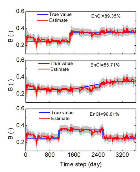
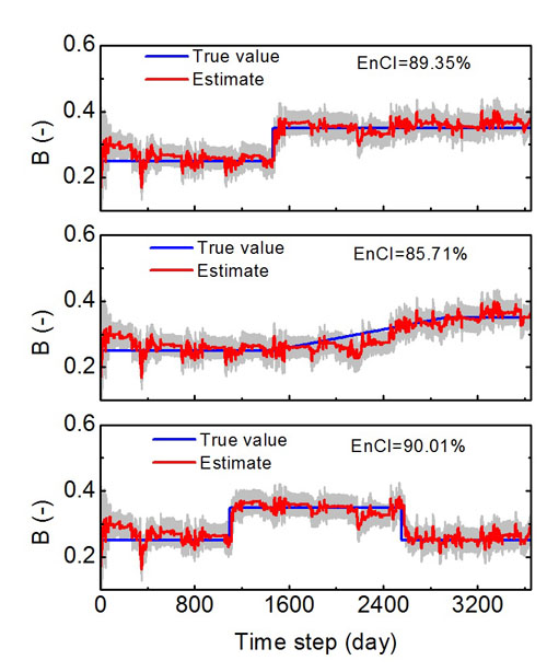
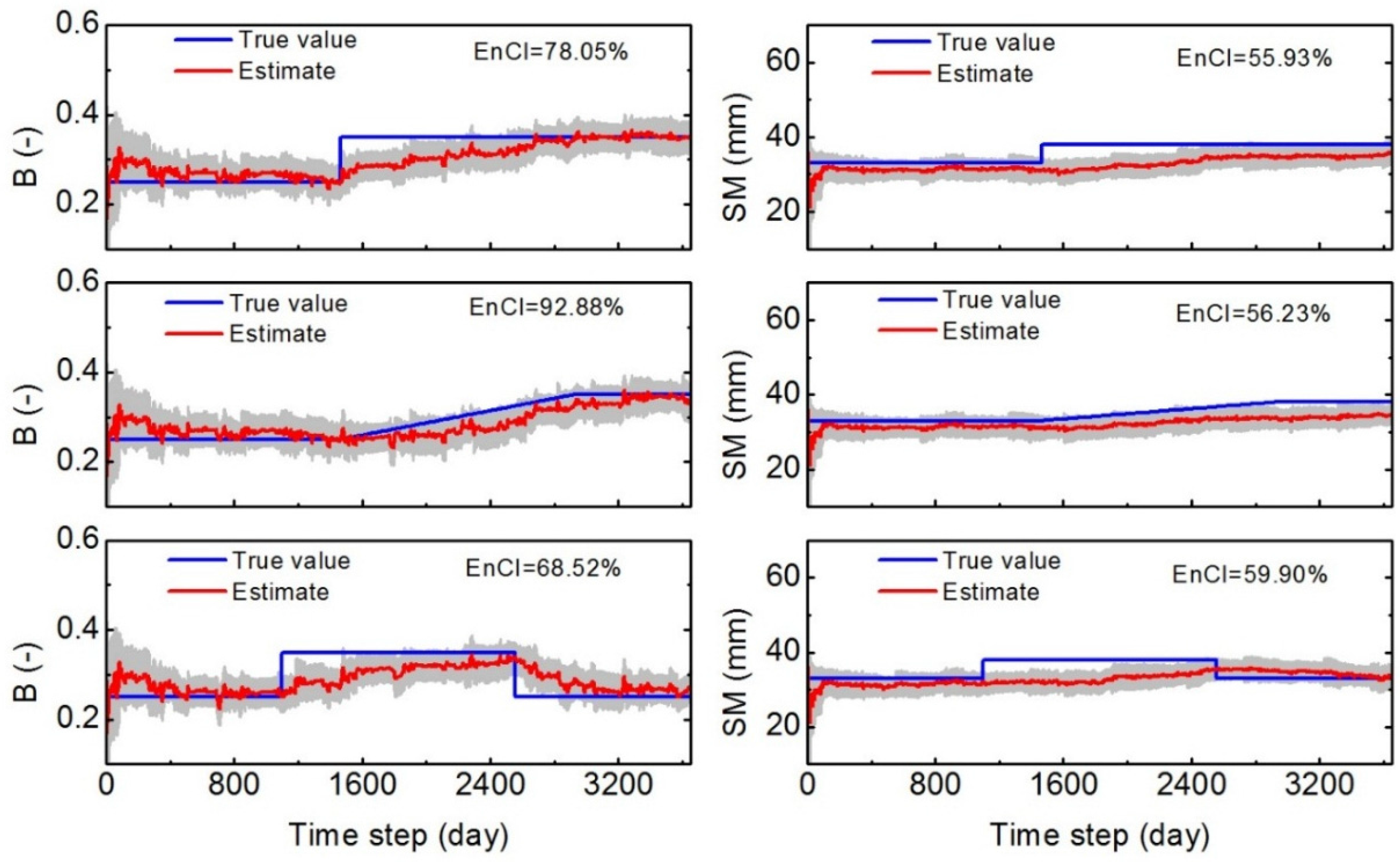
3.2.1. Tracing Changed Parameters

Figure 2 shows the estimates of parameters B and SM for the three non-stationary cases. Although their initial estimates are biased, their sequential estimates can change with the true values when assimilating runoff observations. For instance, parameter B requires approximately 365 assimilation updates. Subsequently, its temporal estimates agree well with the true trajectory. Even when the true trajectory suddenly changes at the 1500th time step for the sudden change case, the estimates immediately respond and arrive at the new stage near the true value of 0.35. For gradual changes, the estimates of the two parameters gradually increase during the 1500th–3000th period to trace their changes. Moreover, the data assimilation provides satisfactory estimates with relative biases less than 5% for the rotational change case, because the true temporal changes of the parameters have been successfully captured, although the pattern is more complex than that of the sudden change case.

Figure 2. Tracing parameter changes for the three non-stationary cases of the sudden (top panel), the gradual (middle panel) and the rotational changes (bottom panel).

Figure 2. Tracing parameter changes for the three non-stationary cases of the sudden (top panel), the gradual (middle panel) and the rotational changes (bottom panel).

In addition to the ensemble mean, the ensemble spread should be examined when tracing the parameter changes. To quantify the coverage of the ensemble spread, we define an ensemble coverage index (EnCI) which is the percentage of the true trajectory of a parameter contained in the 95% ensemble simulation intervals [35]. The EnCI can be visually indicated using the ratio of the blue lines in Figure 2 covered by the grey areas during a specific period. We computed the EnCI for the period of the 366st time step until the end of the simulation, because the first 365 time steps (one year) are generally required to achieve stable estimates.

Figure 2 also shows the EnCIs for the two parameters. For B, the EnCIs in the three cases are approximately 85%; therefore, the ensembles have satisfactory coverage during 85% of the period. For SM, the performance of the coverage depends on the type of change. The EnCI exceeds 90% for the gradual changes, whereas it is less than 70% for the rotational changes. Thus, the estimation of B is more stable than that of SM due to the strong relationship between B and the surface runoff process.

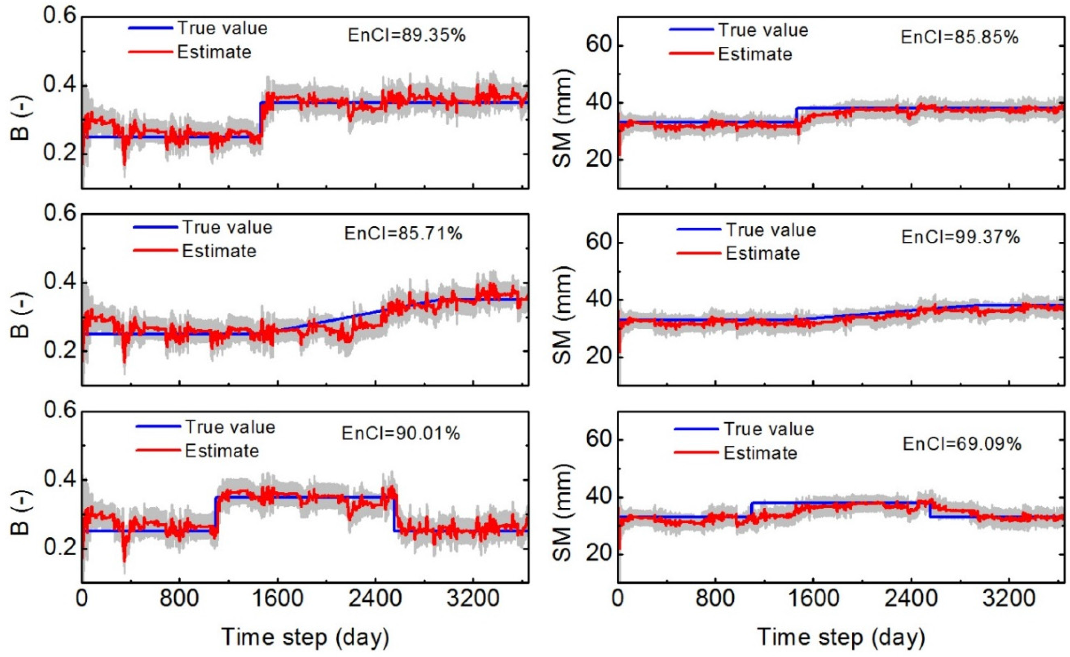
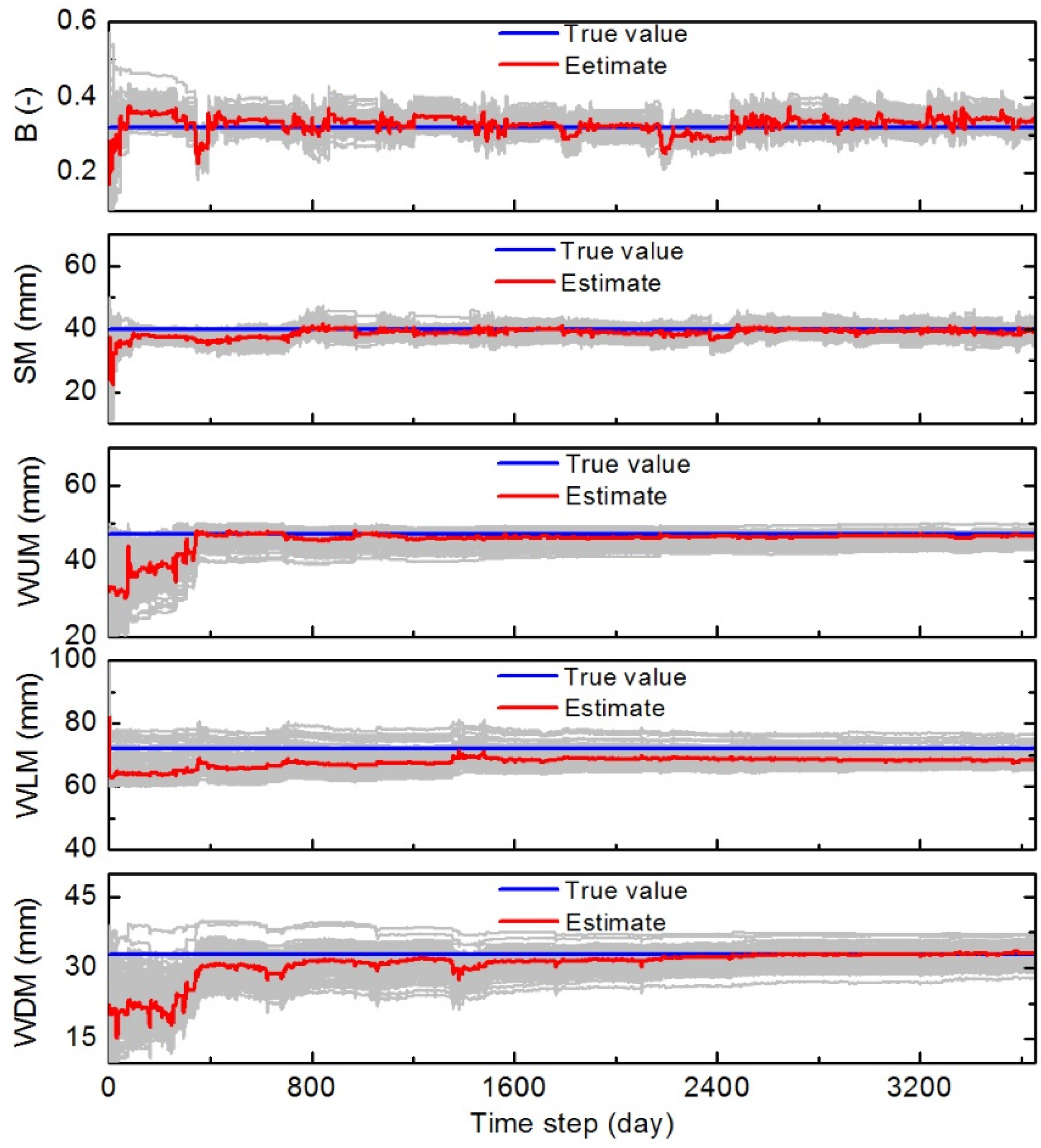
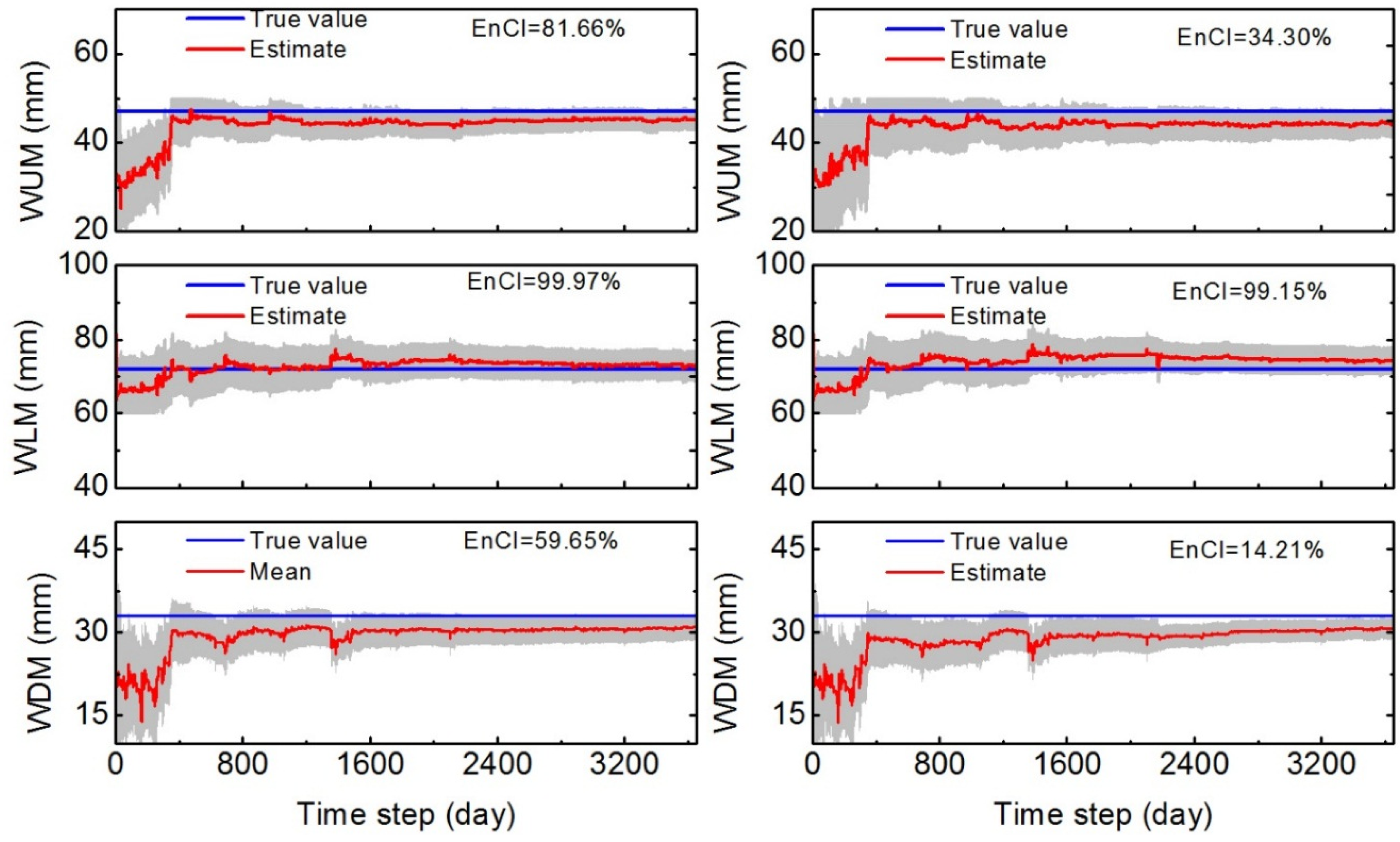
3.2.2. Estimation of Fixed Parameters

In addition to the changing parameters B and SM, we examined the estimation of the other three constant parameters. Figure 3 presents the estimates of WUM, WLM and WDM for gradual and rotational changes. The results of the sudden change case are not shown, because similar or better estimates were obtained for the three parameters. Like the stationary case (Figure 1), the ensemble means of the three parameters acceptably approach their true values. Especially for gradual changes, the estimate of WUM is most accurate among the three parameters even after the 365-step updating, and its EnCI exceeds 99%. For WDM, the estimates are biased to the true trajectory with small EnCIs, because the soil moisture storage capacity of the deep layer (i.e., WUM) has a weak correlation with the surface runoff which is assimilated in this study.

Figure 3. Estimations for WUM, WLM and WDM for two non-stationary cases: the gradual (left) and the rotational (right) changes. The results for the sudden change are not shown. Please note the three parameters do not temporally change since they are more stable than B and SM.

Figure 3. Estimations for WUM, WLM and WDM for two non-stationary cases: the gradual (left) and the rotational (right) changes. The results for the sudden change are not shown. Please note the three parameters do not temporally change since they are more stable than B and SM.

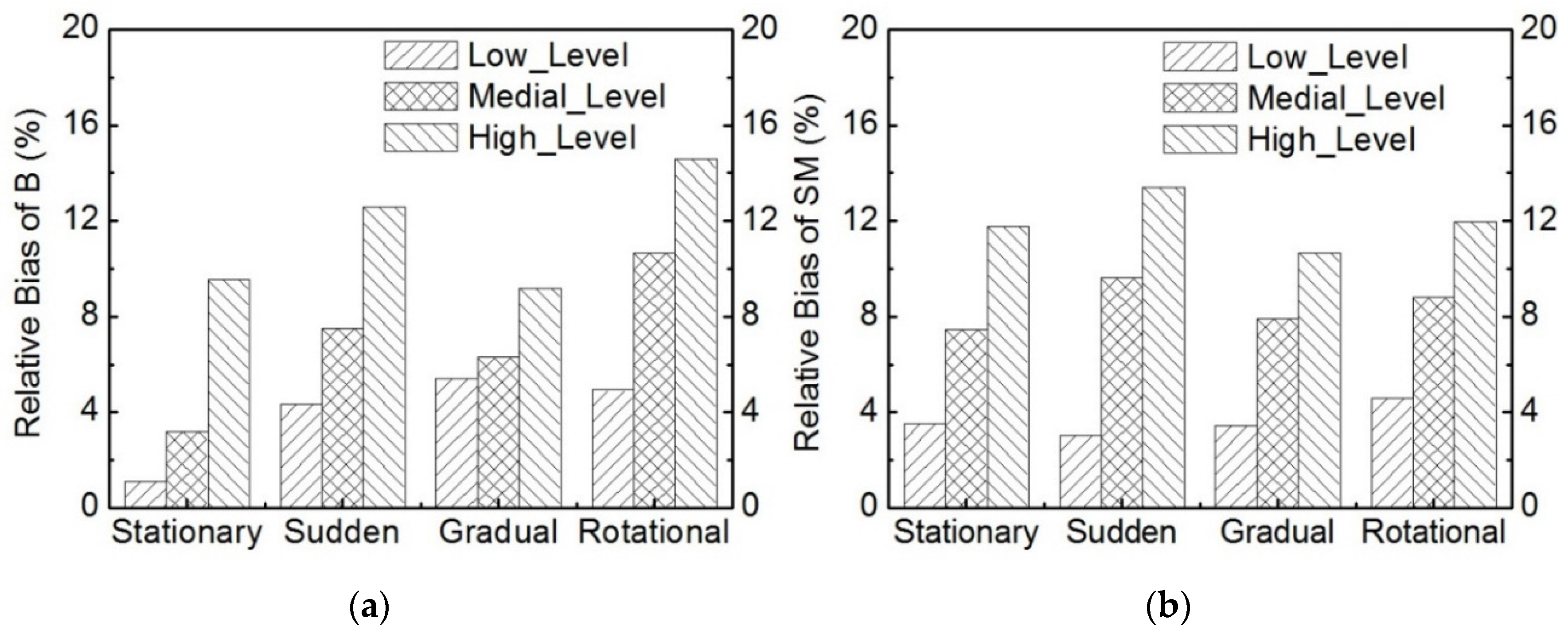
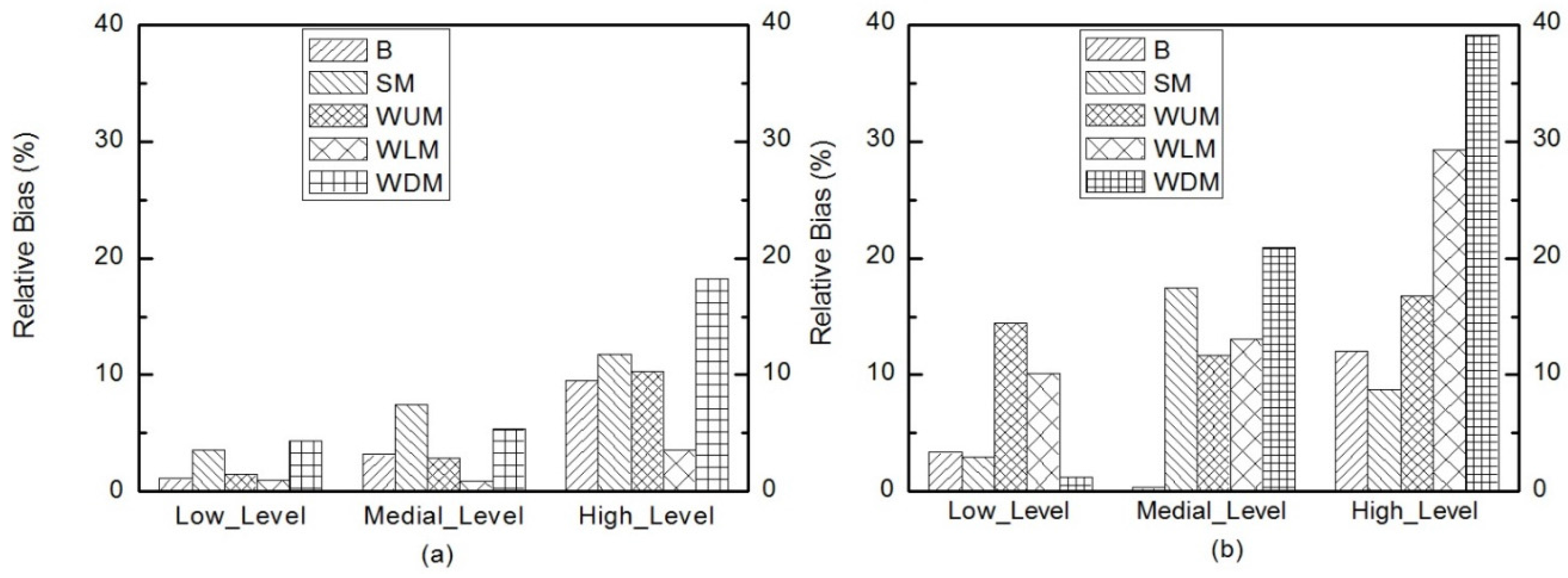
3.3. Effect of the Level of Uncertainties

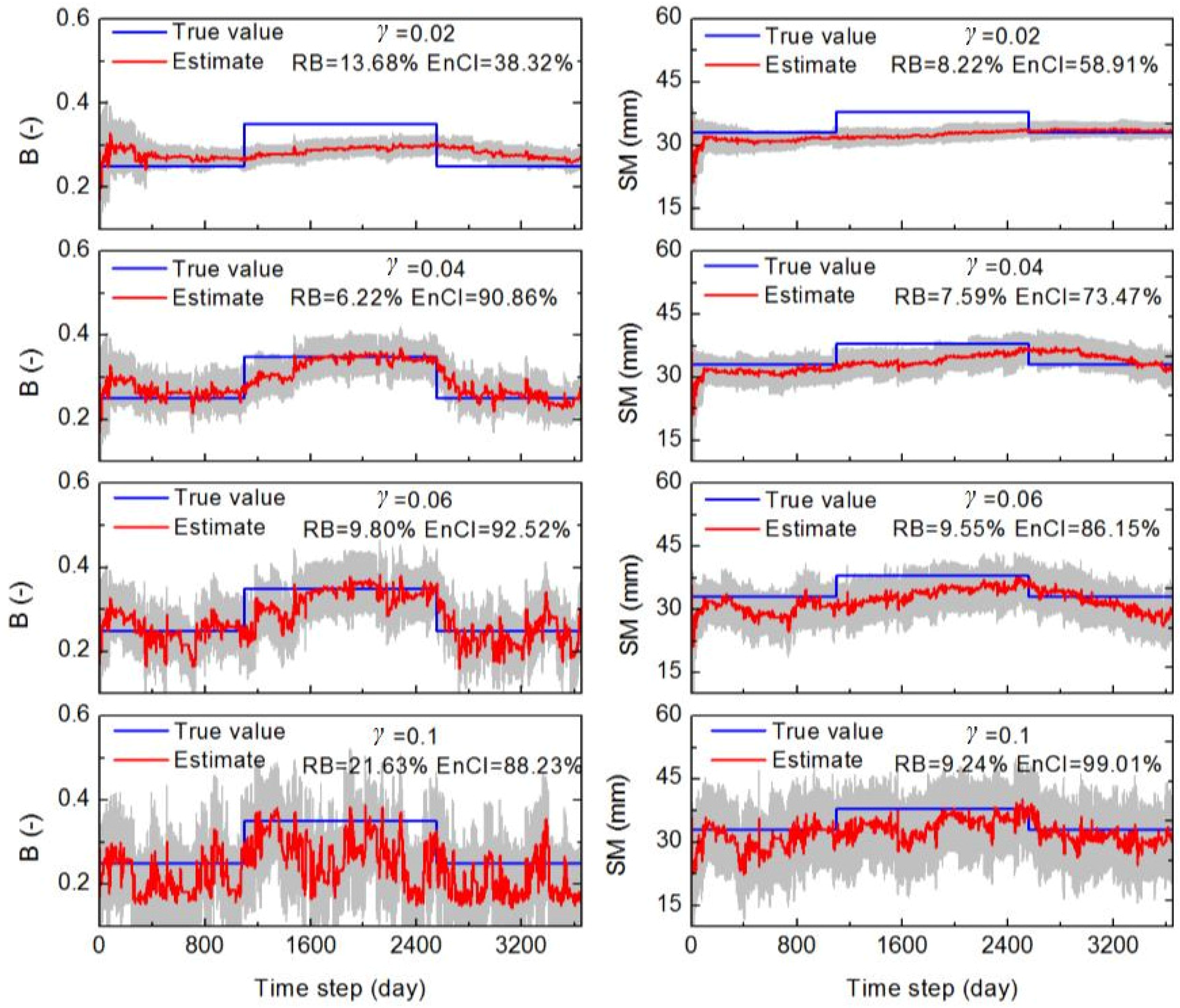
In addition to the above scenario of low-level uncertainties, we designed two other scenarios characterized by larger levels of uncertainties to examine the robustness of the EnKF scheme. These two scenarios feature medial and high levels of errors for rainfall input, modeling and observations (see the Medial_Level and the High_Level scenarios in Table 2).

For the four cases (i.e., one stationary and three non-stationary cases), which are characterized by different levels of uncertainties, we calculated the relative absolute biases based on the estimate series of parameters and their true values. The results of this calculation are shown in Figure 4. The mean relative biases in all cases are below 15%. This is smaller than the levels of uncertainties (Table 2), indicating that data assimilation results in favorable estimates. The bias of parameter estimates directly correlates with the magnitude of uncertainties. Generally, the estimates for the stationary case are more accurate than those for the non-stationary cases. The mean relative bias of the parameter B for the gradual change case do not present the same behavior of other cases. This may be because the estimation of parameter B is not so sensitive to the levels of uncertainties. However, the pattern of biases for the three scenarios is consistent with the other cases. Figure 5 shows the estimates for the three cases under the Medial_Level scenario. In this scenario, the ensemble mean of the parameter B acceptably follows the true trajectories. The estimates for the parameter SM are not so satisfactory with low EnCIs, but its patterns have been successfully depicted. Similar results (not shown) were obtained for the High_Level scenario. Therefore, the EnKF robustly estimates the changes in parameters, but its performance, to some degree, will depend on various levels of uncertainties within modeling and observations.

Figure 4. Relative bias of parameter B (a) and SM (b) estimation under different levels of uncertainties as shown in Table 2.

Figure 4. Relative bias of parameter B (a) and SM (b) estimation under different levels of uncertainties as shown in Table 2.

Figure 5. Tracing parameter changes regarding the three non-stationary cases for the scenario of Medial_Level uncertainty: the sudden change (top panel); the gradual change (middle panel) and the rotational change (bottom panel).

Figure 5. Tracing parameter changes regarding the three non-stationary cases for the scenario of Medial_Level uncertainty: the sudden change (top panel); the gradual change (middle panel) and the rotational change (bottom panel).

3.4. Impact of γ

The coefficient γ in Equation (3) dominates the perturbation of model changes and thereby impacts the accuracy of estimating tracing temporal changes in model parameters. We used four other experiments with γ = 0.02, 0.04, 0.06 and 0.1 to examine the impact of γ. The four experiments were based on the Medial_Level scenario described in Section 3.3, and the other settings were the same as those indicated in Section 2.4.

The rotational changes of the two parameters are shown in Figure 6. The ensemble spread directly correlates with γ, thereby improving the ensemble coverage with respect to the variation of parameters. When γ = 0.02, the ensemble members poorly capture the parameter changes, with low EnCIs (38.32% and 58.91% for parameters B and SM, respectively, as shown in Figure 6). When γ = 0.06, the ensembles achieve acceptable coverage, with EnCIs of 92.52% and 86.15% for parameters B and SM, respectively. In addition to rotational changes, we also examined the sudden and the gradual changes and obtained similar results (not shown).

Figure 6. Tracing parameter changes under different values of γ for the case of the rotational change.

Figure 6. Tracing parameter changes under different values of γ for the case of the rotational change.

Large values of γ improve the coverage of temporal variations of parameters, but this setting may substantially perturb model parameters and consequently cause significant fluctuations in the trajectories of estimates (see Figure 6). For example, when γ = 0.1, sharp fluctuations appear in the estimation of B, with a relative bias of up to 21.63%. Therefore, we recommend a moderate setting for γ (e.g., γ = 0.05) if adequate information regarding the parameter travels and the uncertainties within modeling and observations are not available.

4. Discussion

4.1. Comparison with SCE-UA

The EnKF-based method with a constrained perturbation for model parameters suggests that the parameter travel can be traced under stationary and non-stationary conditions. This method is favorable partly due to its real-time tracing. Moreover, it can account for uncertainties from input forcing, modeling and observations [30]. These merits allow it outperform other optimization methods, which are primarily used for stationary problems. To further distinguish the advantages of this method, we herein employed a widely used global optimization method, i.e., the SCE-UA method [17,18], to estimate the five parameters. We only present the results for the stationary condition, because the SCE-UA is only suitable for parameter estimation under this condition, not the changing condition. In this comparison, please note the EnKF is especially used to estimate model parameters, although it is originally applied to model dynamical processes in a Bayesian framework. In this sense, the comparison between the EnKF and the SCE-UA is reasonable.

To ensure a fair comparison, this estimation was based on the three scenarios (Table 2) in which we intentionally added the uncertainties to the rainfall input, modeling and observations. Please note that these uncertainties are very common in simulation practices. The synthetic observations, i.e., the generated ten-year runoff data, were adopted in this estimation. The SCE-UA method provides optimal estimates for the ten-year period. To evaluate the performance of the SCE-UA, we calculated the relative errors with respect to their true values.

As shown in Figure 7b, the relative errors of the parameters increase with the magnitudes of uncertainties. Especially for High_Level uncertainties, the relative error for WDM is as high as 40%. However, the data assimilation provides very small relative errors (Figure 7a), because the estimates after the 500th updating step are similar to their true values (Figure 1). Although the increasing uncertainties from the rainfall input, modeling and observations decrease the accuracy of the data assimilation to some degree, the relative errors are smaller than those from the SCE-UA method. Notably, the SCE-UA searches the optimal values for model parameters to match the simulated and observed hydrological response, i.e., the runoff in this study, and it attributes all uncertainties in the simulations to the parameters.

Figure 7. Comparison between the the EnKF method (a) andSCE-UA method (b) for parameter estimation.

Figure 7. Comparison between the the EnKF method (a) andSCE-UA method (b) for parameter estimation.

4.2. Implications for Detecting Changes in Watershed Characteristics

Model parameters represent watershed characteristics, such as the soil, topography, LULC and river systems [11]. Although most hydrological models are conceptual, model parameters describe the watershed characteristics in a spatially aggregate manner and are expected to change in response to the dynamics of the watershed behavior [1]. Changes in watershed behavior are usually complex and difficult to be formulated [26]; therefore, changes in the model parameters may show great variety depending on the variability of physical characteristics. This study only focuses on three typical types of parameter changes within synthetic cases. These typical parameter changes could be combined to reflect more complex changes under non-stationary conditions. Thus, the performance of the EnKF-based method indicates that this method may be used to detect the changes in watershed characteristics.

Estimating model parameters for changing conditions remains a significant challenge [19]. Andréassian, et al. presented a distribution-free statistical test to trace gradual changes [57]. Merz et al. employed a consecutive calibration scheme to detect changes in model parameters [26]. During each consecutive period, the model parameters were assumed to be time invariant. However, these studies may not be able to accurately capture sudden changes [57]. The EnKF-based method used in this study has the advantage of updating model parameters in real time or near real time if observations are available, although its performance, to some degree, is impacted by the uncertainties of models and observations. This updating is based on the correlation between hydrological variables and model parameters [34]. Through the sequential updating of model parameters, the timing and magnitudes of changes in watershed characteristics are effectively quantified. Therefore, the hydrological models can adapt to the changing environment and provide more reliable streamflow predictions. Moreover, this real-time updating strategy has the potential to be used in ungauged basins. In such basins, by assimilating a limited number of relevant data from in-situ observations or remote sensing, the model performance could be substantially improved and reaches a reliable hydrological prediction [33,34,35]. This data assimilation strategy is easily used as a continuous simulation for flood frequency predictions since it accounts for various uncertainties and it employs a continuous rainfall-runoff model [58,59,60].

5. Conclusions

Model parameters can change in response to the evolution of watershed characteristics. Estimating changed parameters is important to ensure reliable hydrological predictions under non-stationary conditions. This study employed an EnKF-based method with a constrained parameter evolution scheme to estimate changes in the parameters of the XAJ model based on synthetic experiments. This method features real-time or near real-time updating, accounting for various uncertainties in modeling. In addition to a stationary case, we focused on three typical non-stationary cases and examined the robustness of the EnKF-based method at different levels of uncertainties.

For the stationary case, the ensemble parameter estimates approach their true values after 365 time steps of updating. For the non-stationary cases of the sudden, gradual and rotational changes, the estimates can successfully trace the temporal trends of parameters. Even for a high level of uncertainties, the EnKF-based method yields acceptable results, although the uncertainties from modelling and observations are influential to the performance of data assimilation. We compared the results obtained with the EnKF-based method and the SCE-UA algorithm. SCE-UA shows poor performance to obtain acceptable parameter estimates for the stationary condition if the level of uncertainties increases and it cannot accurately estimate the non-stationary drift of parameters. Although only three typical changes in parameters are discussed in this paper, the real and complex travel of parameters could be reflected by combining these changes. This advantage benefits from real-time updating within the EnKF-based method. Moreover, the parameter estimation can be significantly improved if accurate uncertainties are quantified for rainfall input, modeling and observations [61,62]. The coefficient γ in Equation (3) may influence the ensemble perturbation. We generally suggest specifying a moderate value (e.g., γ = 0.05) when the uncertainties for the rainfall input, modeling and observations are significant.

This study demonstrated the potential of using an EnKF-based method to detect the hydrological impacts of environmental change and adapt the rainfall-runoff model to non-stationary conditions. Despite the success in the four synthetic cases, the EnKF-based method needs to be examined in real watersheds characterized by distinct non-stationarity in the hydrological behavior. Examining the parameter stability of both lumped and physical models and analyzing the rainfall–runoff relationship for such watersheds would be interesting.

References

1. Wagener, T. Can we model the hydrological impacts of environmental change? Hydrol. Process. 2007, 21, 3233–3236. [Google Scholar] [CrossRef]
2. Horton, P.; Schaefli, B.; Mezghani, A.; Hingray, B.; Musy, A. Assessment of climate-change impacts on alpine discharge regimes with climate model uncertainty. Hydrol. Process. 2006, 20, 2091–2109. [Google Scholar] [CrossRef]
3. Huss, M.; Farinotti, D.; Bauder, A.; Funk, M. Modelling runoff from highly glacierized alpine drainage basins in a changing climate. Hydrol. Process. 2008, 22, 3888–3902. [Google Scholar] [CrossRef]
4. Schaefli, B.; Harman, C.; Sivapalan, M.; Schymanski, S. Hess opinions: Hydrologic predictions in a changing environment: Behavioral modeling. Hydrol. Earth Syst. Sci. 2011, 15, 635–646. [Google Scholar] [CrossRef]
5. Wang, W.; Shao, Q.; Peng, S.; Zhang, Z.; Xing, W.; An, G.; Yong, B. Spatial and temporal characteristics of changes in precipitation during 1957–2007 in the haihe river basin, China. Stoch. Environ. Res. Risk Assess. 2011, 25, 881–895. [Google Scholar] [CrossRef]
6. Ghimire, S.R.; Johnston, J.M. Impacts of domestic and agricultural rainwater harvesting systems on watershed hydrology: A case study in the albemarle-pamlico river basins (USA). Ecohydrol. Hydrobiol. 2013, 13, 159–171. [Google Scholar] [CrossRef]
7. Guo, B.; Zhang, J.; Gong, H.; Cheng, X. Future climate change impacts on the ecohydrology of Guishui river basin, China. Ecohydrol. Hydrobiol. 2014, 14, 55–67. [Google Scholar] [CrossRef]
8. Kundzewicz, Z.W. Climate change impacts on the hydrological cycle. Ecohydrol. Hydrobiol. 2008, 8, 195–203. [Google Scholar] [CrossRef]
9. Xie, X.H.; Cui, Y.L. Development and test of swat for modeling hydrological processes in irrigation districts with paddy rice. J. Hydrol. 2011, 396, 61–71. [Google Scholar] [CrossRef]
10. Xie, X.; Liang, S.; Yao, Y.; Jia, K.; Meng, S.; Li, J. Detection and attribution of changes in hydrological cycle over the three-north region of China: Climate change versus afforestation effect. Agric. For. Meteorol. 2015, 203, 74–87. [Google Scholar] [CrossRef]
11. Ehret, U.; Gupta, H.; Sivapalan, M.; Weijs, S.; Schymanski, S.; Blöschl, G.; Gelfan, A.; Harman, C.; Kleidon, A.; Bogaard, T. Advancing catchment hydrology to deal with predictions under change. Hydrol. Earth Syst. Sci. 2014, 18, 649–671. [Google Scholar] [CrossRef]
12. Vaze, J.; Post, D.; Chiew, F.; Perraud, J.-M.; Viney, N.; Teng, J. Climate non-stationarity-validity of calibrated rainfall-runoff models for use in climate change studies. J. Hydrol. 2010, 394, 447–457. [Google Scholar] [CrossRef]
13. Wagener, T.; Sivapalan, M.; Troch, P.A.; McGlynn, B.L.; Harman, C.J.; Gupta, H.V.; Kumar, P.; Rao, P.S.C.; Basu, N.B.; Wilson, J.S. The future of hydrology: An evolving science for a changing world. Water Resour. Res. 2010, 46. [Google Scholar] [CrossRef]
14. Kampf, S.K.; Burges, S.J. Parameter estimation for a physics-based distributed hydrologic model using measured outflow fluxes and internal moisture states. Water Resour. Res. 2007, 43. [Google Scholar] [CrossRef]
15. Xia, Y.; Yang, Z.-L.; Jackson, C.; Stoffa, P.L.; Sen, M.K. Impacts of data length on optimal parameter and uncertainty estimation of a land surface model. J. Geophys. Res. Atmos. 2004, 109. [Google Scholar] [CrossRef]
16. Li, Y.; Ryu, D.; Western, A.W.; Wang, Q.J. Assimilation of stream discharge for flood forecasting: The benefits of accounting for routing time lags. Water Resour. Res. 2013, 49, 1887–1900. [Google Scholar] [CrossRef]
17. Duan, Q.; Sorooshian, S.; Gupta, V. Effective and efficient global optimization for conceptual rainfall-runoff models. Water Resour. Res. 1992, 28, 1015–1031. [Google Scholar] [CrossRef]
18. Duan, Q.Y.; Gupta, V.K.; Sorooshian, S. Shuffled complex evolution approach for effective and efficient global minimization. J. Optim. Theory Appl. 1993, 76, 501–521. [Google Scholar] [CrossRef]
19. Peel, M.C.; Blöschl, G. Hydrological modelling in a changing world. Progress Phys. Geogr. 2011, 35, 249–261. [Google Scholar] [CrossRef]
20. Milly, P.C.D.; Betancourt, J.; Falkenmark, M.; Hirsch, R.M.; Kundzewicz, Z.W.; Lettenmaier, D.P.; Stouffer, R.J. Stationarity is dead: Whither water management? Science 2008, 319, 573–574. [Google Scholar] [CrossRef] [PubMed]
21. Montanari, A.; Young, G.; Savenije, H.; Hughes, D.; Wagener, T.; Ren, L.; Koutsoyiannis, D.; Cudennec, C.; Toth, E.; Grimaldi, S. “Panta rhei—Everything flows”: Change in hydrology and society—The iahs scientific decade 2013–2022. Hydrol. Sci. J. 2013, 58, 1256–1275. [Google Scholar] [CrossRef]
22. Sivapalan, M. Prediction under Change (Puc): Water, Earth and Biota in the Anthropocene, In Proceedings of the AGU Fall Meeting Abstracts, San Francisco, CA, USA, 5–9 December 2011.
23. Sivapalan, M.; Thompson, S.; Harman, C.; Basu, N.; Kumar, P. Water cycle dynamics in a changing environment: Improving predictability through synthesis. Water Resour. Res. 2011, 47. [Google Scholar] [CrossRef]
24. Aich, V.; Liersch, S.; Vetter, T.; Andersson, J.; Müller, E.N.; Hattermann, F.F. Climate or land use?—Attribution of changes in river flooding in the sahel zone. Water 2015, 7, 2796–2820. [Google Scholar] [CrossRef]
25. Merz, R.; Blöschl, G. A regional analysis of event runoff coefficients with respect to climate and catchment characteristics in Austria. Water Resour. Res. 2009, 45. [Google Scholar] [CrossRef]
26. Merz, R.; Parajka, J.; Blöschl, G. Time stability of catchment model parameters: Implications for climate impact analyses. Water Resour. Res. 2011, 47. [Google Scholar] [CrossRef]
27. Aronica, G.; Hankin, B.; Beven, K. Uncertainty and equifinality in calibrating distributed roughness coefficients in a flood propagation model with limited data. Adv. Water Resour. 1998, 22, 349–365. [Google Scholar] [CrossRef]
28. Castaings, W.; Dartus, D.; le Dimet, F.X.; Saulnier, G.M. Sensitivity analysis and parameter estimation for distributed hydrological modeling: Potential of variational methods. Hydrol. Earth Syst. Sci. 2009, 13, 503–517. [Google Scholar] [CrossRef] [Green Version]
29. Vrugt, J.A.; Gupta, H.V.; Bouten, W.; Sorooshian, S. A shuffled complex evolution metropolis algorithm for optimization and uncertainty assessment of hydrologic model parameters. Water Resour. Res. 2003, 39. [Google Scholar] [CrossRef]
30. Liu, Y.; Gupta, H.V. Uncertainty in hydrologic modeling: Toward an integrated data assimilation framework. Water Resour. Res. 2007, 43. [Google Scholar] [CrossRef]
31. Kumar, S.V.; Reichle, R.H.; Peters-Lidard, C.D.; Koster, R.D.; Zhan, X.; Crow, W.T.; Eylander, J.B.; Houser, P.R. A land surface data assimilation framework using the land information system: Description and applications. Adv. Water Resour. 2008, 31, 1419–1432. [Google Scholar] [CrossRef]
32. Moradkhani, H.; Sorooshian, S.; Gupta, H.V.; Houser, P.R. Dual state–parameter estimation of hydrological models using ensemble kalman filter. Adv. Water Resour. 2005, 28, 135–147. [Google Scholar] [CrossRef]
33. Xie, X.; Zhang, D. Data assimilation for distributed hydrological catchment modeling via ensemble kalman filter. Adv. Water Resour. 2010, 33, 678–690. [Google Scholar] [CrossRef]
34. Xie, X.H.; Zhang, D.X. A partitioned update scheme for state-parameter estimation of distributed hydrologic models based on the ensemble kalman filter. Water Resour. Res. 2013, 49, 7350–7365. [Google Scholar] [CrossRef]
35. Xie, X.; Meng, S.; Liang, S.; Yao, Y. Improving streamflow predictions at ungauged locations with real-time updating: Application of an enkf-based state-parameter estimation strategy. Hydrol. Earth Syst. Sci. 2014, 18, 3923–3936. [Google Scholar] [CrossRef]
36. Zhao, R.J. The xinanjiang model applied in china. J. Hydrol. 1992, 135, 371–381. [Google Scholar]
37. Zhao, R.; Liu, X.; Singh, V. The xinanjiang model. In Comput. Model. Watershed Hydrol; Water Resources Publications: Littleton, CO, USA, 1995; pp. 215–232. [Google Scholar]
38. Ren, L.; Huang, Q.; Yuan, F.; Wang, J.; Xu, J.; Yu, Z.; Liu, X. Evaluation of the xinanjiang model structure by observed discharge and gauged soil moisture data in the hubex/game project. Iahs Publ. 2006, 303, 153–163. [Google Scholar]
39. Hu, C.; Guo, S.; Xiong, L.; Peng, D. A modified xinanjiang model and its application in northern China. Nordic Hydrol. 2005, 36, 175–192. [Google Scholar]
40. Bao, H.J.; Zhao, L.N.; He, Y.; Li, Z.J.; Wetterhall, F.; Cloke, H.L.; Pappenberger, F.; Manful, D. Coupling ensemble weather predictions based on tigge database with grid-xinanjiang model for flood forecast. Adv. Geosci. 2011, 29, 61–67. [Google Scholar] [CrossRef]
41. Xu, H.; Xu, C.-Y.; Chen, H.; Zhang, Z.; Li, L. Assessing the influence of rain gauge density and distribution on hydrological model performance in a humid region of China. J. Hydrol. 2013, 505, 1–12. [Google Scholar] [CrossRef]
42. Li, Z.J.; Xin, P.L.; Tang, J.H. Study of the Xinanjiang model parameter calibration. J. Hydrol. Eng. 2013, 18, 1513–1521. [Google Scholar]
43. Zhang, D.; Zhang, L.; Guan, Y.; Chen, X.; Chen, X. Sensitivity analysis of xinanjiang rainfall-runoff model parameters: A case study in Lianghui, Zhejiang Province, China. Hydrol. Res. 2012, 43, 123–134. [Google Scholar] [CrossRef]
44. Song, X.M.; Kong, F.Z.; Zhan, C.S.; Han, J.W.; Zhang, X.H. Parameter identification and global sensitivity analysis of Xin’anjiang model using meta-modeling approach. Water Sci. Eng. 2013, 6, 1–17. [Google Scholar]
45. Evensen, G. Data Assimilation: The Ensemble Kalman Filter; Springer Science & Business Media: Berlin, Germany, 2009. [Google Scholar]
46. Chen, H.; Yang, D.; Hong, Y.; Gourley, J.J.; Zhang, Y. Hydrological data assimilation with the ensemble square-root-filter: Use of streamflow observations to update model states for real-time flash flood forecasting. Adv. Water Resour. 2013, 59, 209–220. [Google Scholar] [CrossRef]
47. Ghil, M. Data assimilation in meteorology and oceanography. Adv. Geophys. 1991, 33, 141–266. [Google Scholar]
48. Shi, L.; Zeng, L.; Zhang, D.; Yang, J. Multiscale-finite-element-based ensemble kalman filter for large-scale groundwater flow. J. Hydrol. 2012, 468–469, 22–34. [Google Scholar] [CrossRef]
49. Reichle, R.H.; McLaughlin, D.B.; Entekhabi, D. Hydrologic data assimilation with the ensemble kalman filter. Mon. Weather Rev. 2002, 130, 103–114. [Google Scholar] [CrossRef]
50. Evensen, G. The ensemble kalman filter: Theoretical formulation and practical implementation. Ocean Dyn. 2003, 53, 343–367. [Google Scholar] [CrossRef]
51. Evensen, G.; van Leeuwen, P.J. An ensemble kalman smoother for nonlinear dynamics. Mon. Weather Rev. 2000, 128, 1852–1867. [Google Scholar] [CrossRef]
52. Liu, F. Bayesian Time Series: Analysis Methods Using Simulation-Based Computation. Ph.D Thesis, Institutes of Statistics and Decision Science, Duke University, Duke, NC, USA, May 2000. [Google Scholar]
53. Clark, M.P.; Rupp, D.E.; Woods, R.A.; Zheng, X.; Ibbitt, R.P.; Slater, A.G.; Schmidt, J.; Uddstrom, M.J. Hydrological data assimilation with the ensemble kalman filter: Use of streamflow observations to update states in a distributed hydrological model. Adv. Water Resour. 2008, 31, 1309–1324. [Google Scholar] [CrossRef]
54. Chu, W.; Gao, X.; Sorooshian, S. Improving the shuffled complex evolution scheme for optimization of complex nonlinear hydrological systems: Application to the calibration of the sacramento soil-moisture accounting model. Water Resour. Res. 2010, 46. [Google Scholar] [CrossRef]
55. Evans, W.E.; Friday, E.W., Jr. Multilevel Calibration Strategy for Complex Hydrologic Simulation Models; US Department of Commerce, National Oceanic and Atmospheric Administration, National Weather Service: Washington, DC, USA, 1989. [Google Scholar]
56. Sorooshian, S.; Duan, Q.; Gupta, V.K. Calibration of rainfall-runoff models: Application of global optimization to the sacramento soil moisture accounting model. Water Resour. Res. 1993, 29, 1185–1194. [Google Scholar] [CrossRef]
57. Andréassian, V.; Parent, E.; Michel, C. A distribution-free test to detect gradual changes in watershed behavior. Water Resour. Res. 2003, 39. [Google Scholar] [CrossRef]
58. Blazkova, S.; Beven, K. A limits of acceptability approach to model evaluation and uncertainty estimation in flood frequency estimation by continuous simulation: Skalka catchment, Czech Republic. Water Resour. Res. 2009, 45. [Google Scholar] [CrossRef]
59. Calver, A.; Stewart, E.; Goodsell, G. Comparative analysis of statistical and catchment modelling approaches to river flood frequency estimation. J. Flood Risk Manag. 2009, 2, 24–31. [Google Scholar] [CrossRef]
60. Grimaldi, S.; Petroselli, A.; Serinaldi, F. A continuous simulation model for design-hydrograph estimation in small and ungauged watersheds. Hydrol. Sci. J. 2012, 57, 1035–1051. [Google Scholar] [CrossRef]
61. Crow, W.T.; Reichle, R.H. Comparison of adaptive filtering techniques for land surface data assimilation. Water Resour. Res. 2008, 44. [Google Scholar] [CrossRef]
62. Crow, W.T.; van Loon, E. Impact of incorrect model error assumptions on the sequential assimilation of remotely sensed surface soil moisture. J. Hydrometeorol. 2006, 7, 421–432. [Google Scholar] [CrossRef]