A New Spatiotemporal Risk Index for Heavy Metals: Application in Cyprus

Abstract

The main aim of this research was to improve risk mapping of heavy metals by taking account of erosion effects. A new spatiotemporal index, namely the G2met index, is introduced, with integration of pre-existing methodologies (Hakanson, EPM, and G2). The G2met index is depicted as a series of risk maps for each heavy metal on a month-time step. The southern part of Cyprus Island was selected as a study area. Concentration of major heavy metals was extracted with soil sampling in a grid of 5350 sites. Rainfall, vegetation, soil, land use, topographic, and hydrologic data were collected from existing European or global databases (WorldClim, BioBar, REDES, ESDAC, CORINE, ASTER GDEM, and USGS). A large number of regional-scale risk maps (with 500-m cell size) were created: one for each heavy metal and totally per month and annually; in addition, choropleth maps in terms of statistics per river basin were produced for every metal. Generally, the G2met maps resulted in different spatial patterns in comparison to those depicted by the Hakanson index alone.

1. Introduction

Heavy metal contamination of soils is regarded as a potential hazard of food safety and public health. Exposure to polluted soils may take place in different ways, e.g., through the consumption of vegetables grown on contaminated soils, drainage of rich in heavy metals waste disposal, dust inhalation, etc.

The off-site transport of chemicals bounded to sediments may cause pollution and silting of water resources. Sediment is defined as the loose sand, clay, silt or other soil particles that settle at the bottom of a body of water [1] and is considered as a habitat and major nutrient source for aquatic organisms. Sediment analysis is important in evaluating qualities of total ecosystem of a water body in addition to water sample analysis, because it reflects the long term quality situation independent of the current inputs [2].

Contamination of soil and water is indirectly referred to by numerous existing legislative policies in the European Union, such as the Directives regarding the disposal of wastes (Landfill, Mining waste), the Sewage sludge Directives and directives regarding the application of chemicals, the Regulation for Plant protection and Pesticide use Directives, the Industrial emissions Directive, the Water Framework Directive, and the Air quality Framework Directive.

A variety of methods has been developed to estimate heavy metal accumulation into soils and sediments. Among them, pollution risk indices are considered to be a powerful tool for ecological geochemistry assessment [3]. In 1969, Müller introduced the Geoaccumulation Index [4], originally used with river bottom sediments and more recently for soil contamination [5]; the same index was used as an evaluation tool for pollution from an abandoned mine by [6], or for comparing differences between current and preindustrial concentrations [7]. The Average Daily Intake (ADI) is an index focusing on the impact component of risk assessment, while Monte Carlo simulations have been applied in order to reduce distribution uncertainties, using data from different sources [8]. Pollution Index (PI) is an index defined as the ratio of the metal concentration to the background concentration of the corresponding metal [7] and is equivalent to the contamination factor of metal as defined by [9]. In his review, Gong et al. [3] report also several indices as different expressions of the fuzzy logic theory applied in risk assessment [10].

A range of risk definitions can be found in the literature [11]. A common attribute in all these definitions, however, is the probabilistic nature of the risk, which in mathematical terms is defined usually as a multiplicative equation [12]:

RISK = Threat × Exposure × Impact

(1)

According to [13], quite commonly risk assessment is lacking of spatial analysis, whereas is based only on static measurements of pollutant concentrations in some critical sites. However, as Lahr et al. [14] notify, spatial analysis help interpretation of potential impacts of environmental stressors. Especially, considering that remote areas may be connected to the pollution sources in ways that are not immediately apparent [15]. Moreover, is important for sustainable territorial planning and prevention of natural disasters [16].

Risk maps can be of different types, such as contamination maps, exposure maps, or hazard maps. Critical parameters of mapping specifications with regard to the detail, minimum mapping unit (MMU), value ranging or classification and symbolization, are discussed by [17]. The approach for the estimation of the exposure component of risk is different for point from non-point (diffused) pollution sources and for different scales as well. Risk mapping for soil heavy metal pollution from mines (a diffused case) in China was applied by [8]. For a point-source pollution problem (olive mill wastewaters), Karydas et al. [18] has followed a multi-scale approach through pathway analysis.

In all currently used indices for heavy metals, however, there is lack of a component which would convincingly express the effect of soil erosion processes in the potential sediment loads. Defined as the process of detachment and transport of soil material by wind or water [19], the soil erosion processes (soil loss, deposition downwards, and sedimentation in surface waters) [20] could be considered as the exposure component of risk assessment for heavy metals and -at the same time-, the linking mechanism between pollution sources and receptors. According to [21], sedimentation data analysis could also support impact assessment of distant human activities.

The main aim of this research was to improve risk assessment of heavy metals potentially reaching surface water courses and water bodies. Improvement could be achieved by a proposed new risk index which would:

• Account for soil erosion processes, thus linking heavy metal concentrations in soils with downstream potential sediment loads.
• Be dynamic (temporal), in terms of providing assessments in regular short time steps (and not simply static lumped values).
• Combine all required risk assessment components, i.e., threat, vulnerability, and impact.
• Be spatial in terms of providing standardized risk maps.

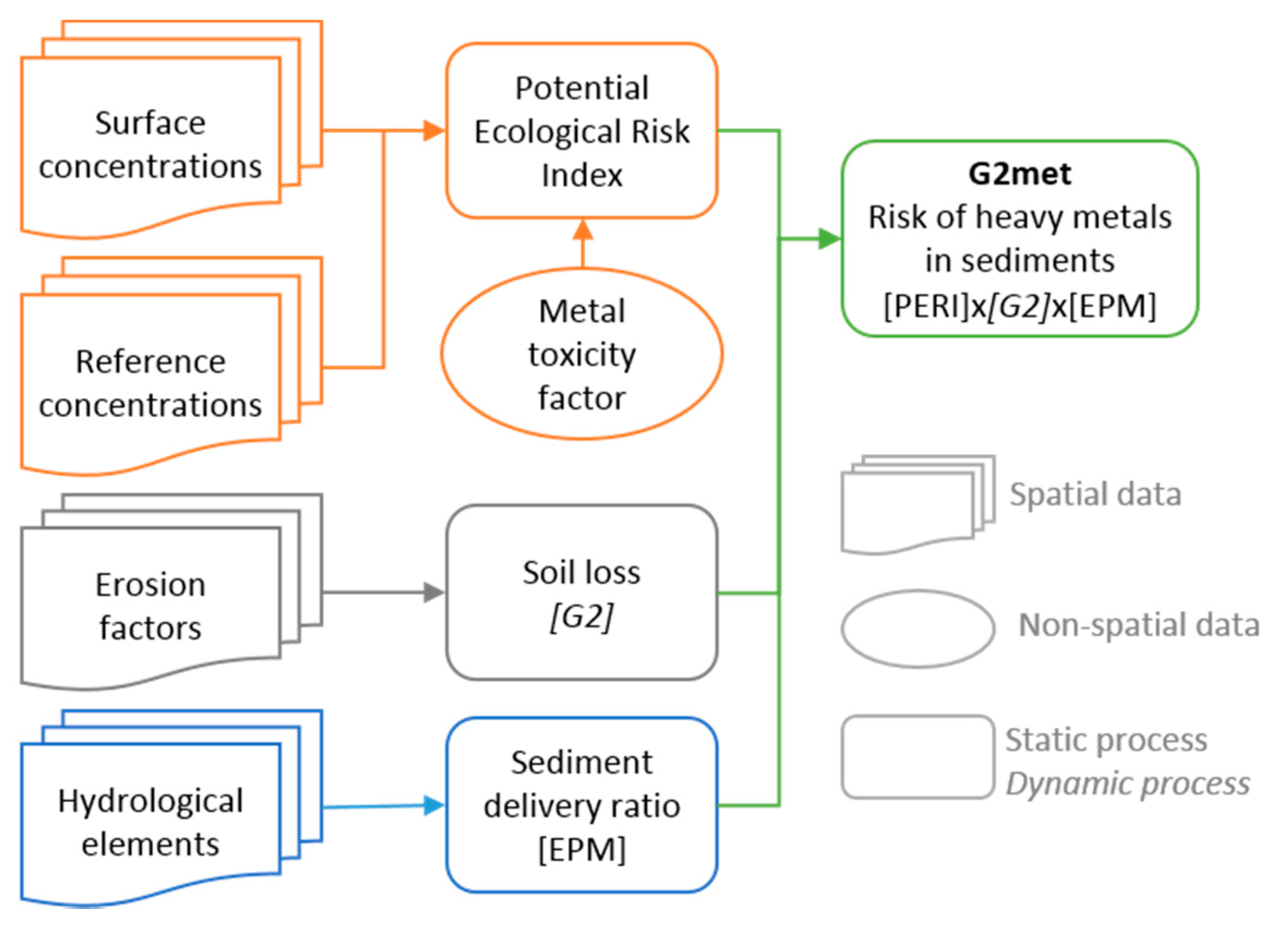
2. Index definition

The development of the new risk index for heavy metals was achieved through the conceptual, algorithmic, and spatial integration of three pre-existing risk assessment methods, each dedicated to a very particular role (Figure 1):

• The Potential Ecological Risk Index (PERI, or Hakanson index) for the estimation of the risk associated with the concentration of heavy metals in soils or sediments [9].
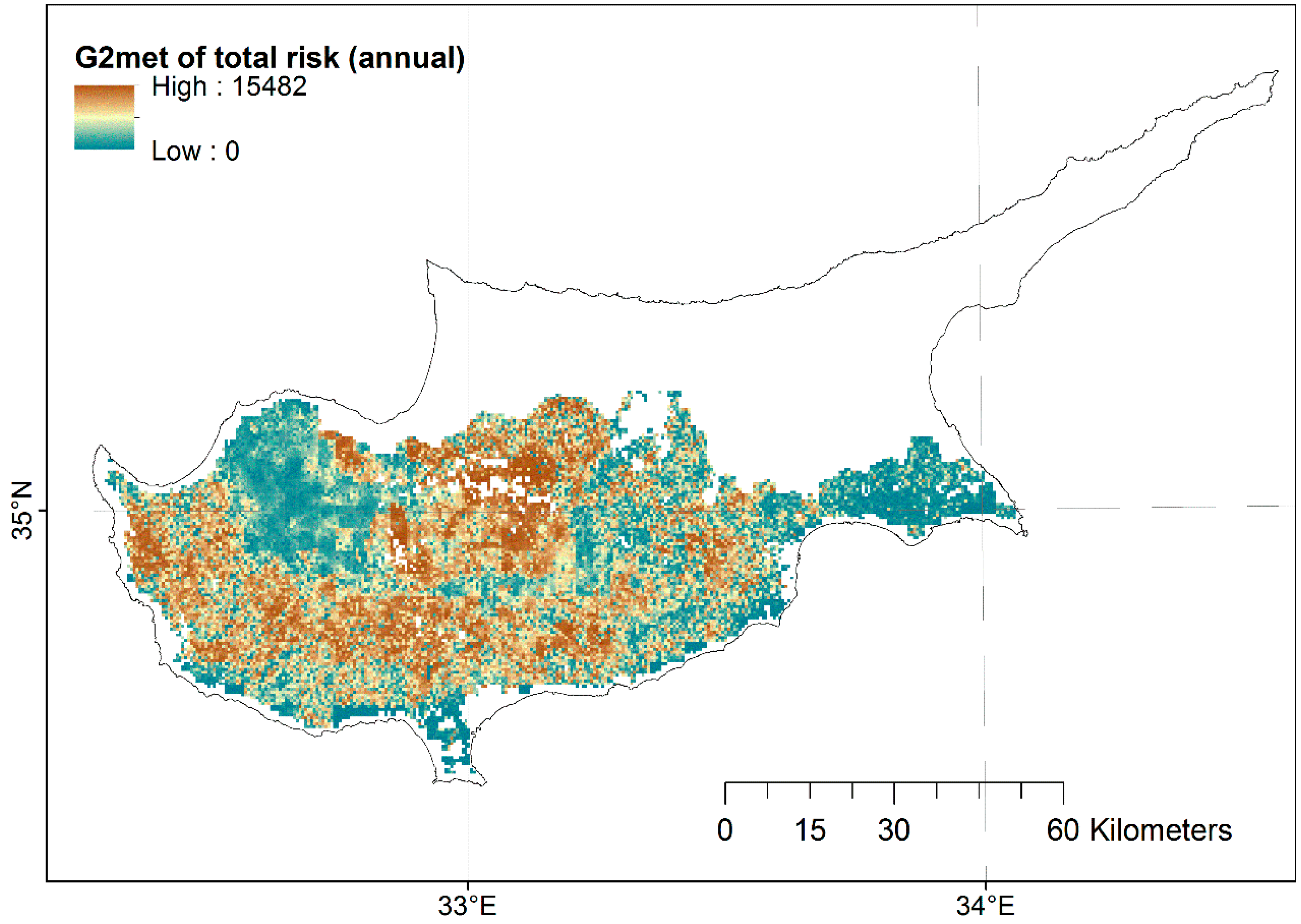
• The G2 model for mapping risk of soil loss on a monthly-time scale [22].
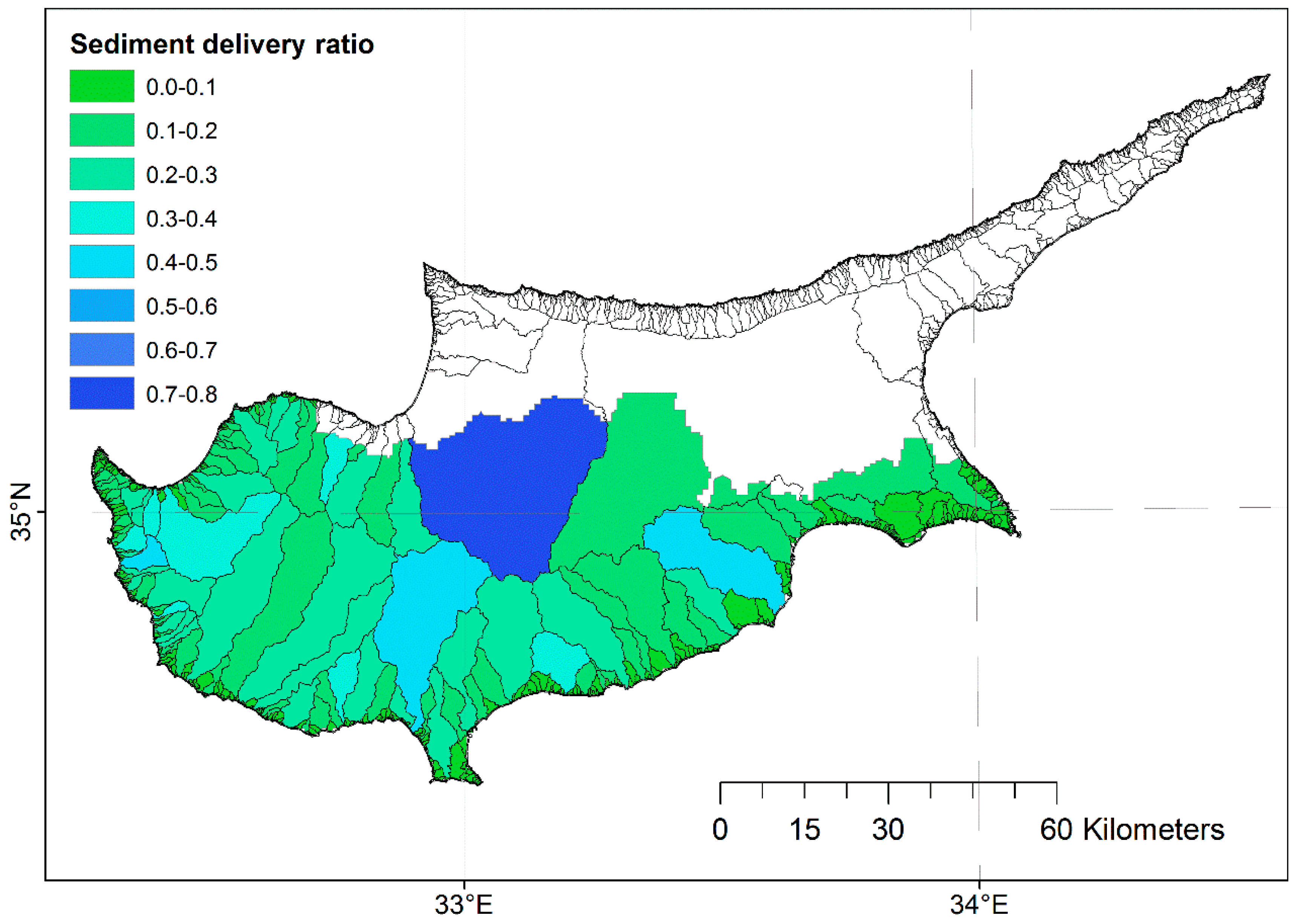
• The Erosion Potential Model (EPM, or Gavrilovic) and specifically its sedimentation component, for estimating sediment delivery ratio (SDR) on a basin scale [23].

Figure 1. An overview of the methodology for calculating the G2met index.

Figure 1. An overview of the methodology for calculating the G2met index.

The new index measures the risk of a specific heavy metal (or all of them) to reach surface waters. The new index is named “G2met” and is defined mathematically as follows:

$$G2met(m)=c·H_m·E·SDR$$

(2)

where G2met(m): spatial risk index for metal m during a specific month (dimensionless); H_m: Hakanson index of metal m or the total index value for all heavy metals found in a site (dimensionless); E: soil loss (t·ha⁻¹) at the site; and SDR: sediment delivery ratio of the river basin in which the contaminated and eroded site belongs (decimal in the range 0–1); c = 1·ha·t⁻¹ (dimensional constant).

Defining G2met as a product of the Hakanson index and erosion effect, G2met values remain comparable with Hakanson values, thus indicating the effect of erosion in terms of a numerical multiplier. As is derived from Equation (2), a G2met value would be equal with the H_m value when one ton of polluted soil per ha is transferred to the stream course as sediment.

The G2met index is expressed in terms of a time series of risk maps for each heavy metal alone and entirely, therefore is by default a spatiotemporal risk index. In their review on pollutant risk mapping [14] conclude that risk maps can substantially assist in environmental risk analysis and communication.

The new index follows the fundamental principle of the environmental risk theory, according to which risk is a combined output of three components: threat (or frequency), exposure, and impact (or vulnerability) [10,14]. In the composition of the G2met index, threat is represented by the term $C_f^i$ of the Hakanson index (called “contamination factor”), while impact is represented by the term $T_f^i$ of the Hakanson index (called “toxicity factor”); therefore, the Hakanson index provides by default the two out of three risk components for heavy metals.

As a consequence, the only missing component of the specific risk is “exposure” of the hazard to the environment, in terms of probability to connect an existing threat with potential impact on ecosystems. This missing component is provided—in G2met—by the incorporated erosion factors, i.e., soil loss (E) and sediment delivery ratio (SDR). A parameter or process bridging sources and receptors in large scale risk mapping is required for an integrative risk assessment at the basin scale. Moreover, incorporation of erosion processes in pollution risk by heavy metals is in line also with the nature of this risk as a non-point source pollution risk. According to the US Environmental Protection Agency (EPA), nonpoint source pollution generally results from land runoff, precipitation, atmospheric deposition, drainage, seepage or hydrologic modification [24].

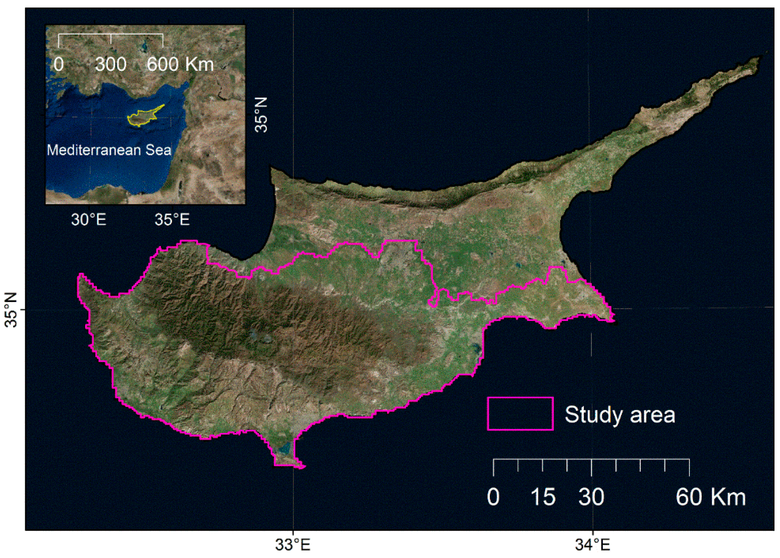
3. Application in Cyprus

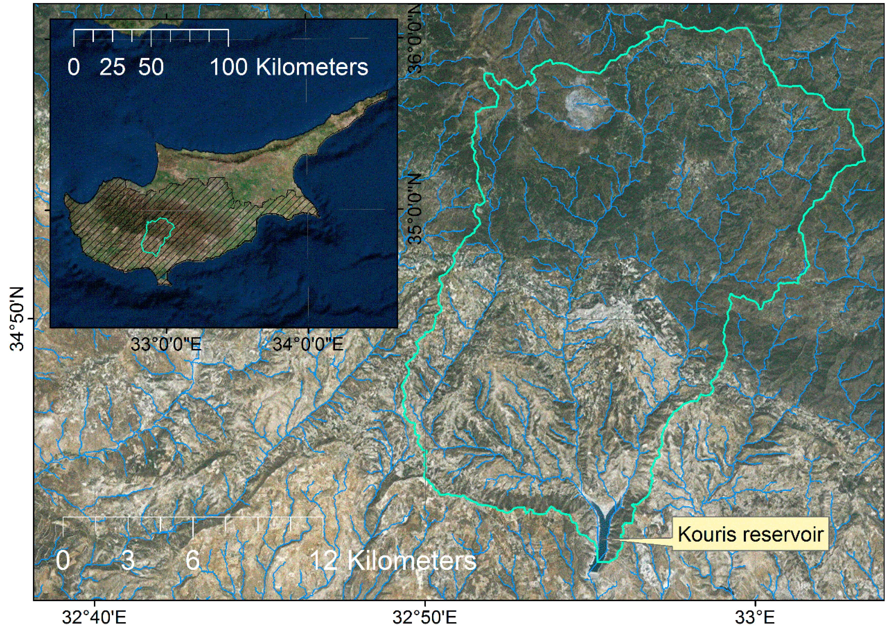
3.1. Study Area

The Mediterranean island of Cyprus, which is rich in heavy metals and highly risky to erosion, was selected as a study area. Cyprus is the third largest Mediterranean island—and the biggest in the eastern Mediterranean basin—with a surface area of 9251 km². However, the current study was restricted to the southern part of the island due to inaccessibility to required heavy metal data in the northern part. The extent of the study area covers mainly the south-west and the south-central part of the island resulting in an extent of about 5947 km² (Figure 2).

Figure 2. Cyprus Island is located in the Eastern Mediterranean Basin (see inset); the study area was addressed in the southern part of the island (basemap from ArcMap©).

Figure 2. Cyprus Island is located in the Eastern Mediterranean Basin (see inset); the study area was addressed in the southern part of the island (basemap from ArcMap©).

The soil characteristics of Cyprus reflect the steep topography in the mountainous areas, the rapid tectonic uplift and the relatively young age of the terrane. Massive red soils are observed in various exposures from the upper parts of Troodos Range (in the center of the island; highest peak: Mt. Olympus, 1951 m) to the coastal plain (center, east, and south-east). According to the soil survey (2009) of the Land Use/Cover Area frame Survey (LUCAS), five main topsoil classes are recognized: regosols, cambisols, calcisols, leptosols and luvisols [25]. The Phosphorous content in topsoils is lower than 20 mg·kg⁻¹ (average value), the average pH value is 7.4, and the average Nitrogen percentage content is estimated to 0.13% (1.3 g·kg⁻¹).

Considering the volcanic geologic feature of Cyprus, the high slope terrain and the intensification of the human activities during the last decades, examination of environmental risk from heavy metal contamination and high potential of these polluted soils to be eroded and mobilized [26] should be urgently assessed. According to the geochemical Atlas of Cyprus, geochemical values are mostly related to parent lithology and subsequent regolith processes, since there is strong correlation between top soil and sub soil geochemical values. However, sediment quality assessment is more complex than water quality assessment alone, due to several site-specific parameters. Stabilization and other forms of long-term self-containing barriers, could reduce the mobility and availability of critical pollutants [27].

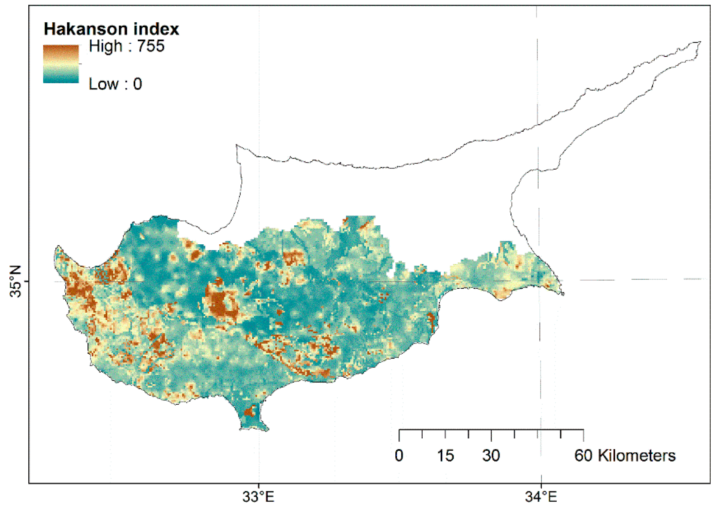
3.2. Calculation of the Hakanson Index

Hakanson’s ecological risk index (RI) evaluates the potential ecological risks associated with the metal contaminant concentrations found in soils and sediment samples [9]. The index reflects not only the single ecological risk of individual contaminants, but also addresses the integrated ecological-toxicological effects of multiple pollutants through dividing the ecological risk levels of soil contamination and is calculated using the following equations:

$$C_f^i=\frac{C_s^i}{C_r^i}$$

(3)

$$E_r^i=T_f^i·C_f^i$$

(4)

$$RI=\mathrm{\sum }\left(E_r^i\right)=\mathrm{\sum }\left(T_f^i·\frac{C_s^i}{C_r^i}\right)$$

(5)

where $C_f^i$: contamination factor of metal i; $C_s^i$: measured concentration of metal i in the sample, with the following metals used in this method: Cu, Ni, Pb, As, Zn, Hg, Cd, and Cr; $C_r^i$: background (reference) concentration of metal i in the sediments; $E_r^i$: specific metal potential ecological risk factor; $T_f^i$: biological toxicity factor for a single metal, which is used to reflect the toxic levels of heavy metals and the water sensitive to the metal contamination; and RI: potential ecological risk index, describing a comprehensive value of multiple pollutants. Referring to [9], the following $T_f^i$ values were employed in the current study: Cd = 30; Cr = 2; Cu = 5; Ni = 5; Pb = 5; Zn = 1; Hg = 40; and As = 10. The parameter RI can be divided into four grades: Low risk (RI ≤ 50), Moderate risk (50 < RI ≤ 100), Considerable risk (100 < RI ≤ 200) and High risk (RI > 200).

The heavy metal concentration of major heavy metals (Cd, Cr, Cu, Ni, Pb, Zn, Hg, and As) was extracted by the national geochemical map of Cyprus. The soil and sediment monitoring has been conducted for the period May 2006 to January 2009 at the high sampling density of 1 site per 1 km², taking samples of top soil (0–25 cm depth) and sub soil (50–75 cm depth) from a grid of over 5350 sites across the study area. The results of the soil analysis are presented in detail by [28]. Inverse-distance weighting (IDW) was used to generate the geochemical maps. The selected IDW model had a grid-cell size of 0.33 km, a distance weighting exponent of 1.6 and a maximum search radius from the center of each grid-cell of 2 km, in order to preserve the point data characteristics of the sample and limit propagation of anomalies from points with very high or low values [28].

Table 1 shows mean concentrations of heavy metal found in the seven main geologic formations, representing 78% of Cyprus extent. All units showed similar heavy metal range with the exception of Basal group that experiences higher Zn (109.8 mg kg⁻¹) and Cu (167.5 mg kg⁻¹) content. Industrial zones, urban areas and some other locations display higher contents of Pb, Cu, Hg, Sn, and Zn, especially in topsoil.

Table 1. Heavy metal surface mean concentrations in various geologic units of Cyprus (in mg·kg⁻¹).

Geologic Formation	Extent (%)	As	Cd	Cr	Ni	Pb	Zn	Hg	Cu
Pakhna	15.4	5.6	0.4	57.8	62.5	12.7	44.0	0.034	39.7
Alluvium or Colluvium	9.1	5.0	0.2	60.3	55.4	7.4	50.6	0.035	57.1
Fanglomerate	6.0	5.7	0.2	55.6	44.4	8.4	53.1	0.025	43.5
Nicosia	6.5	7.0	0.2	50.4	42.1	9.6	56.0	0.031	43.6
Lefkara	10.3	3.0	0.3	36.8	47.0	6.4	39.1	0.032	51.8
Basal Group	6.4	3.2	0.2	53.8	42.1	4.2	109.8	0.035	167.5
Sheeted Dykes (Diabase)	18.0	1.6	0.1	51.2	38.1	2.5	68.8	0.030	195.7
Average	–	4.9	0.3	73.7	111	11	67	0.030	87.9

Table 1. Heavy metal surface mean concentrations in various geologic units of Cyprus (in mg·kg⁻¹).

Geologic Formation	Extent (%)	As	Cd	Cr	Ni	Pb	Zn	Hg	Cu
Pakhna	15.4	5.6	0.4	57.8	62.5	12.7	44.0	0.034	39.7
Alluvium or Colluvium	9.1	5.0	0.2	60.3	55.4	7.4	50.6	0.035	57.1
Fanglomerate	6.0	5.7	0.2	55.6	44.4	8.4	53.1	0.025	43.5
Nicosia	6.5	7.0	0.2	50.4	42.1	9.6	56.0	0.031	43.6
Lefkara	10.3	3.0	0.3	36.8	47.0	6.4	39.1	0.032	51.8
Basal Group	6.4	3.2	0.2	53.8	42.1	4.2	109.8	0.035	167.5
Sheeted Dykes (Diabase)	18.0	1.6	0.1	51.2	38.1	2.5	68.8	0.030	195.7
Average	–	4.9	0.3	73.7	111	11	67	0.030	87.9

Reference, or background, or quality reference value refers to the natural concentration of an element or a substance in soils that have not been modified by anthropogenic impacts [29]. The heavy metals concentration of the sub soil data was used to establish the reference values in each geologic formation of Cyprus based on the statistical analysis (75th percentile of the frequency distribution of the data series [30]) of the laboratory results of samples. The weighted average background value of all examined metals (Table 2) are lower than the values suggested by [31]. Chromium, Copper and Nickel values are found to have higher values than those reported by JRC/EU [31] in some geologic units. For instance higher copper values were observed in Basal, Sheeted Dykes and pillow lavas. High background chromium values were found in Serpentine and sheared Serpentine soils. The background values were estimated lower for Cyprus in comparison to Brazilian soils (Table 2) with the exception of the Ni background value [29].

In order to keep the uncertainty of background metal computations low: (1) Estimated values were compared to those established in various international case studies (Table 2); (2) The ratio of top-soil versus sub-soil data of Ni (a heavy metal mainly originated by pedogenic and in general non- anthropogenic processes) was checked and estimated close to one (average value 0.98), thus indicating subsoils data sufficient to estimate background values; and (3) Strong dependency of the geochemical atlas of Cyprus on geologic formations was evaluated through systematic observations [28].

Table 2. Heavy metal reference concentrations in the various geologic units (in mg kg⁻¹).

Reference Sources	As	Cd	Cr	Ni	Pb	Zn	Hg	Cu
Weighted average Background values for Cypriot soils	0.36	0.01	18.95	39.3	0.66	7.51	0.001	11.62
Min weighted average Background for Cypriot soils	<0.1	<0.1	<5.0	<0.1	<0.1	<0.1	<0.01	<0.1
Μax weighted average Background for Cypriot soils	3.42	0.12	161.7	420.1	9.88	81.5	0.012	229.6
Threshold values for soils of pH > 7	–	1.5	100	70	100	200	1.0	100
Reference values for Brazilian soils	–	<LQ	47.9	8.7	15.3	22.4		18.2

Table 2. Heavy metal reference concentrations in the various geologic units (in mg kg⁻¹).

Reference Sources	As	Cd	Cr	Ni	Pb	Zn	Hg	Cu
Weighted average Background values for Cypriot soils	0.36	0.01	18.95	39.3	0.66	7.51	0.001	11.62
Min weighted average Background for Cypriot soils	<0.1	<0.1	<5.0	<0.1	<0.1	<0.1	<0.01	<0.1
Μax weighted average Background for Cypriot soils	3.42	0.12	161.7	420.1	9.88	81.5	0.012	229.6
Threshold values for soils of pH > 7	–	1.5	100	70	100	200	1.0	100
Reference values for Brazilian soils	–	<LQ	47.9	8.7	15.3	22.4		18.2

Using Equations (3)–(5), a set risk maps according to the Hakanson index were produced from interpolated concentration layers (surface and reference concentrations) and toxicity constant values for all reported heavy metals in the study area and for their accumulative risk (named “total”) (Figure 3). Due to the fact that Cd and Hg have distinctly high biological toxicity factors, their contribution to the total risk is significantly higher than the rest of the metals; together they contribute by about 66%.

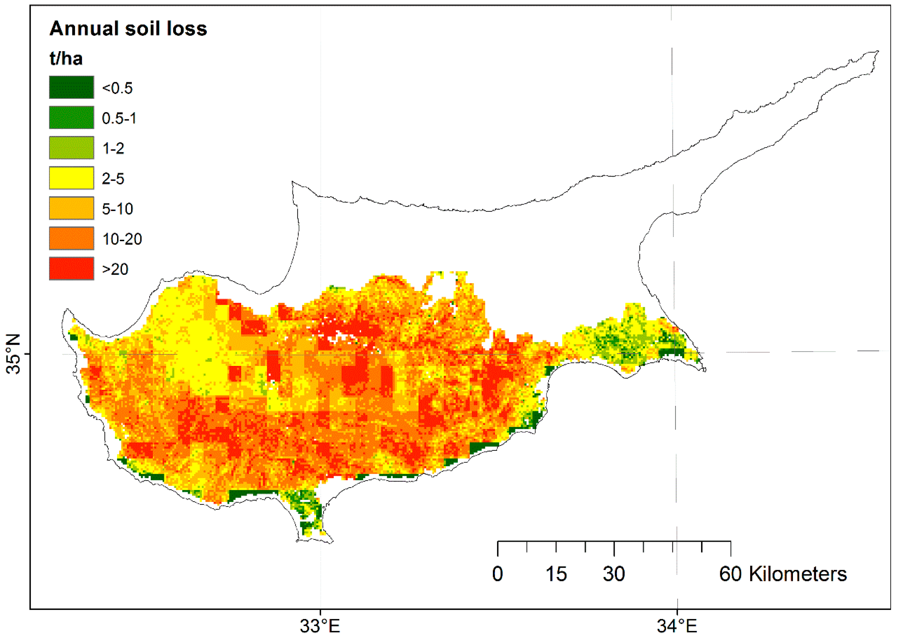
3.3. Soil Loss Mapping Using the G2 model

The G2 model inherits its main principles from the Universal Soil Loss Equation (USLE). According to [32], G2 is classified as a “Watershed to landscape–Pathway type–Averaged–Empirical” model. Soil loss values are calculated by G2 using the following equation [33]:

$$E=\frac{R}{V}·S·\frac{T}{I}$$

(6)

where E: soil loss (t·ha⁻¹); R: rainfall erosivity (MJ·cm·ha⁻¹·h⁻¹); V: vegetation retention (V≥1; dimensionless); S: soil erodibility (t·ha·h·MJ⁻¹·ha⁻¹·cm⁻¹); T: topographic influence (T ≥ 0; dimensionless); I: slope intercept (1 ≤ I ≤ 2; dimensionless). All units are defined by the empirical equations of USLE for R and S (the latter denoted by K in USLE).

Figure 3. The total Hackanson index raster map created with stratified interpolation (cell size: 500 m; value ranging: histogram equalization; mean value: 37.086).

Figure 3. The total Hackanson index raster map created with stratified interpolation (cell size: 500 m; value ranging: histogram equalization; mean value: 37.086).

G2 is designed to run in a GIS environment provided that one spatial layer is prepared for S, one for T, and one for I; whereas, 12 spatial layers are required for R and another 12 spatial layers are required for V (i.e., one layer per month for each of R and V). Since 2010 when it was first introduced, G2 has evolved into a set of alternative formulas for the calculation of all erosion factors. The G2 model has been made available to decision makers by the Soil Erosion section of the European Soil Data Center (ESDAC) of the Joint Research Center, through provision of guidance, datasets and support [33].

The monthly R-factor layers of Cyprus were calculated from 35 precipitation stations with 30-min rainfall data, which are part of the Rainfall Erosivity Database of Europe (REDES) [34]. According to [35], the spatial interpolation of monthly erosivity point data use the precipitation data from the WorldClim database as covariates [36] and in accordance to the Generalized Adaptive Model (GAM) [37].

Estimation of the V-factor by G2 is based on the combination of two parameters: the fraction of the surface covered by vegetation (Fcover) and the land use effect (LU). Fcover layers were downloaded for years 2011–2013 from: catftp.vgt.vito.be (last accessed: 06-03-2015) [38,39]. The LU values were calculated by compiling CORINE 2006 Land Cover database with the Gavrilovic (or EPC) model empirical data [26].

The S-factor layer resulted from the interpolation of 89 soil samples using the cubist regression model [40], where S at samples was calculated with the original USLE K-equation [41].

For the estimation of topographic influence on erosion (T), the method of [42] was applied. Required hydrological and topographic parameters were calculated from a mosaic of digital elevation model (derived from set of six tiles) downloaded from the ASTER GDEM/METI-NASA geoportal.

The slope intercept factor expresses the potential of an alternating landscape to intercept rainfall runoff by reducing the slope length. Two Landsat 8 images covering Cyprus and acquired during summer 2013 and 2014, were downloaded from the United States Geological Survey (USGS) portal [43]. The images were mosaicked prior to their processing.

The output of the G2 model for the study area comprises a set of 12 monthly soil loss layers at 100-m resolution. The average annual erosion rate in the study area was estimated at 11.75 t·ha⁻¹ with a standard deviation of 10.17 t·ha⁻¹ (Figure 4). Three seasons of different risk level can be discriminated: a high risk season during October–December (with averaged monthly rates larger than 1·t·ha⁻¹), three medium risk seasons during May–July, January, and September (with averaged monthly rates between 0.5 and 1·t·ha⁻¹), and two low risk seasons during February–April and August (with averaged monthly rates smaller than 0.5·t·ha⁻¹).

Figure 4. The annual soil loss map of Cyprus (cell size: 100 m; value ranging: user defined).

Figure 4. The annual soil loss map of Cyprus (cell size: 100 m; value ranging: user defined).

In an erosion study in Yialias basin, located in central Cyprus (111 km², outlet next to Potamia village), a mean value of 20.95 t·ha⁻¹·yr⁻¹ is reported by [44]. In the same basin, G2 resulted in a mean value of 10.58 t·ha⁻¹·year⁻¹, which is close to the mean value of the entire study area (10.32 t·ha⁻¹·year⁻¹). However, there are not any systematic experimental data in Cyprus, to which the created maps could be compared; therefore, the results could not be validated against ground truth data.

3.4. Sediment Delivery Ratio Using the EPM

EPM comprises a soil loss and a soil sedimentation component. The model was developed in the Morava river basin (Serbia) and later was implemented in other areas of Europe. The equations used for calculating SDR are the following [24]:

$$SDR=\frac{\sqrt{P·Z}·(L_p+L_s)}{(L_p+10)·A}$$

(7)

where SDR: sediment delivery ratio (decimal in range 0–1), P: basin perimeter (km), Z: difference of mean altitude from minimum altitude of the basin (km), Lp: total length of the primary stream segments (highest order in the specific basin) (km), Ls: total length of the secondary stream segments (km), and A: basin extent (km²).

All the hydrologic elements, i.e., river basins and stream networks, required to extract input parameter to Equation (7), were mapped using the D8 methodology. The stream network was mapped with a flow accumulation threshold set at 500 after trial and error, while stream order was defined using the Strahler method [45].

The data source for extracting all hydrological and topographic information (e.g., Z) was an ASTER GDEM (global digital elevation model), the same used for extracting the required parameters for T factor calculation in soil loss mapping with G2. The implementation of the EPM equation in the spatial domain resulted in a per basin averaged SDR value of 0.28 with a maximum value of 0.71 (Figure 5).

Figure 5. Choropleth map of the sediment delivery ratio (SDR) per river basin (value ranging: 0.1 step; mean value: 0.28).

Figure 5. Choropleth map of the sediment delivery ratio (SDR) per river basin (value ranging: 0.1 step; mean value: 0.28).

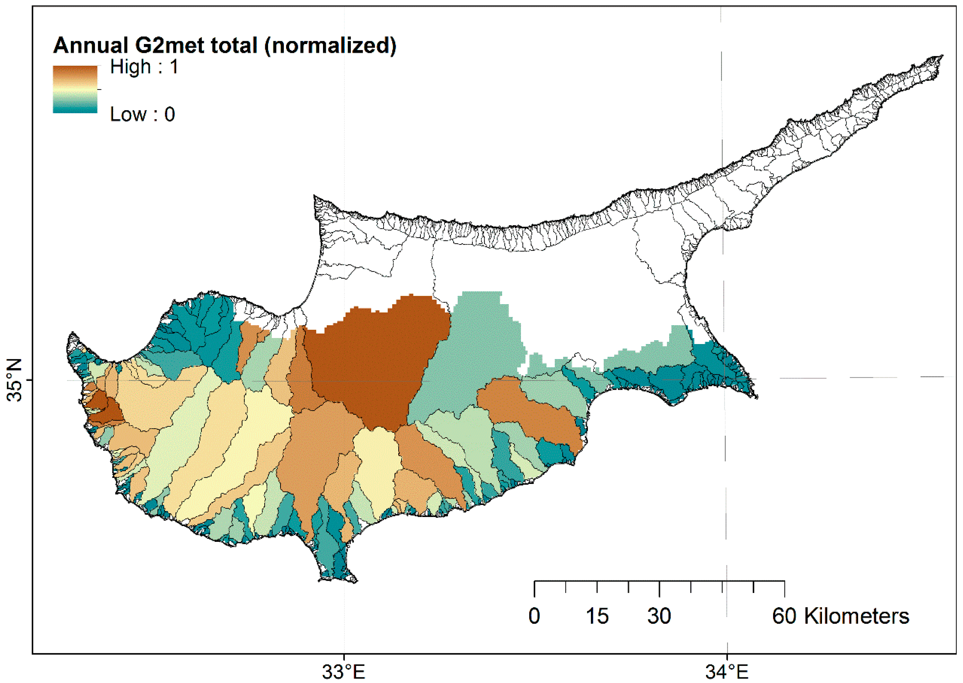
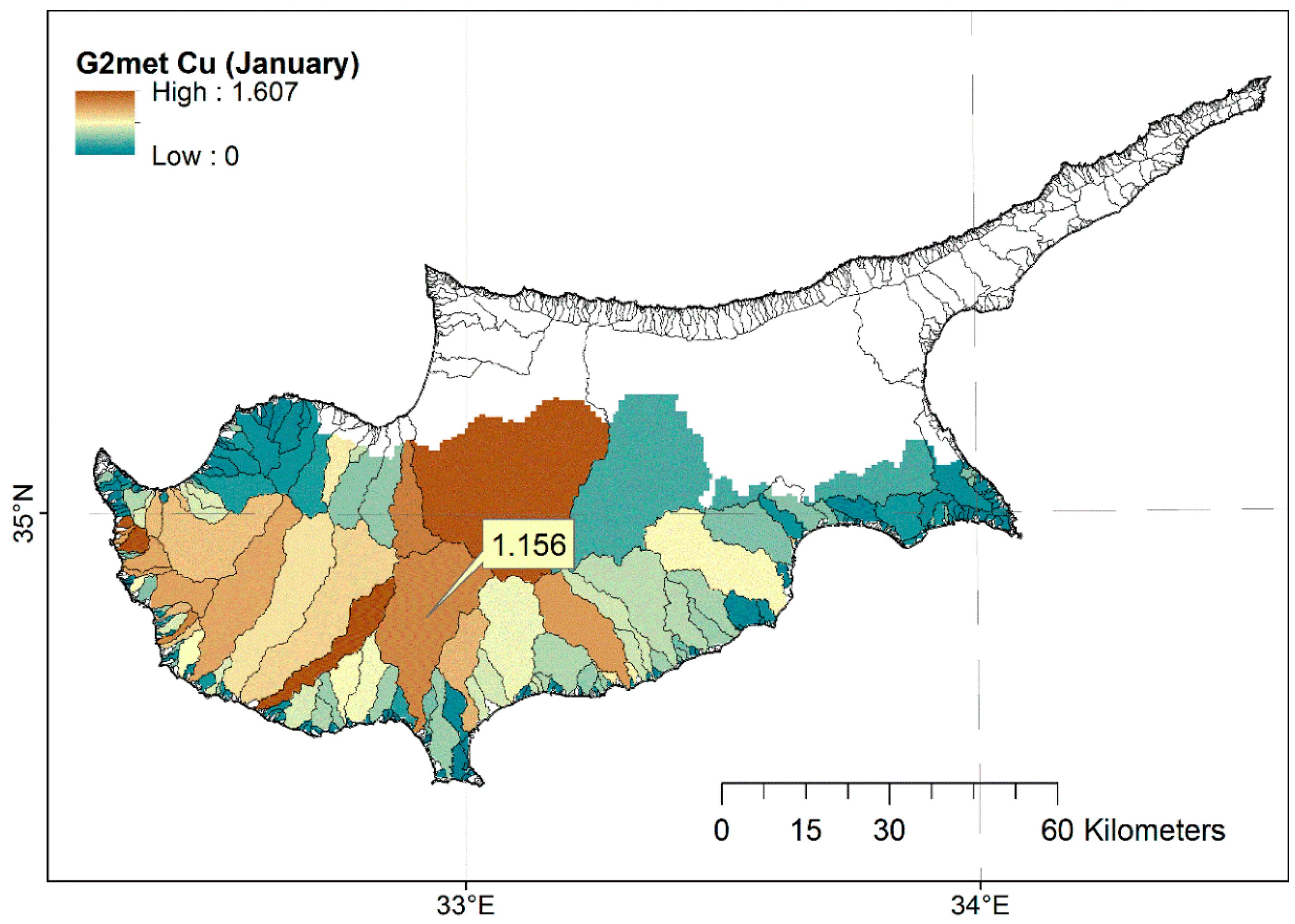
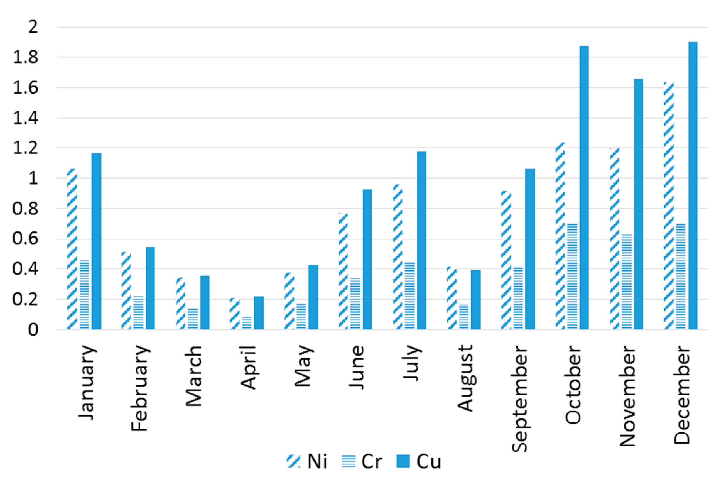
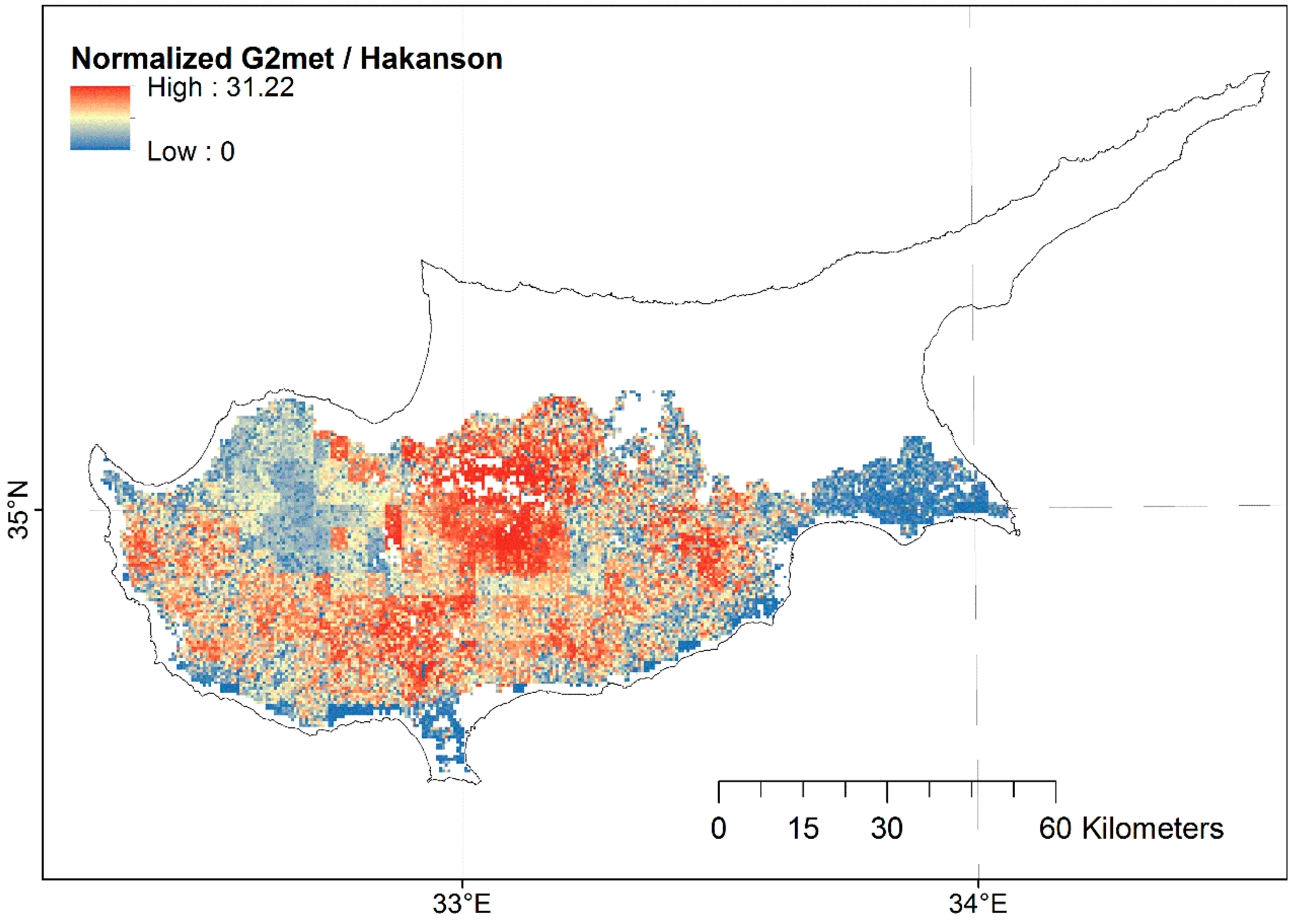
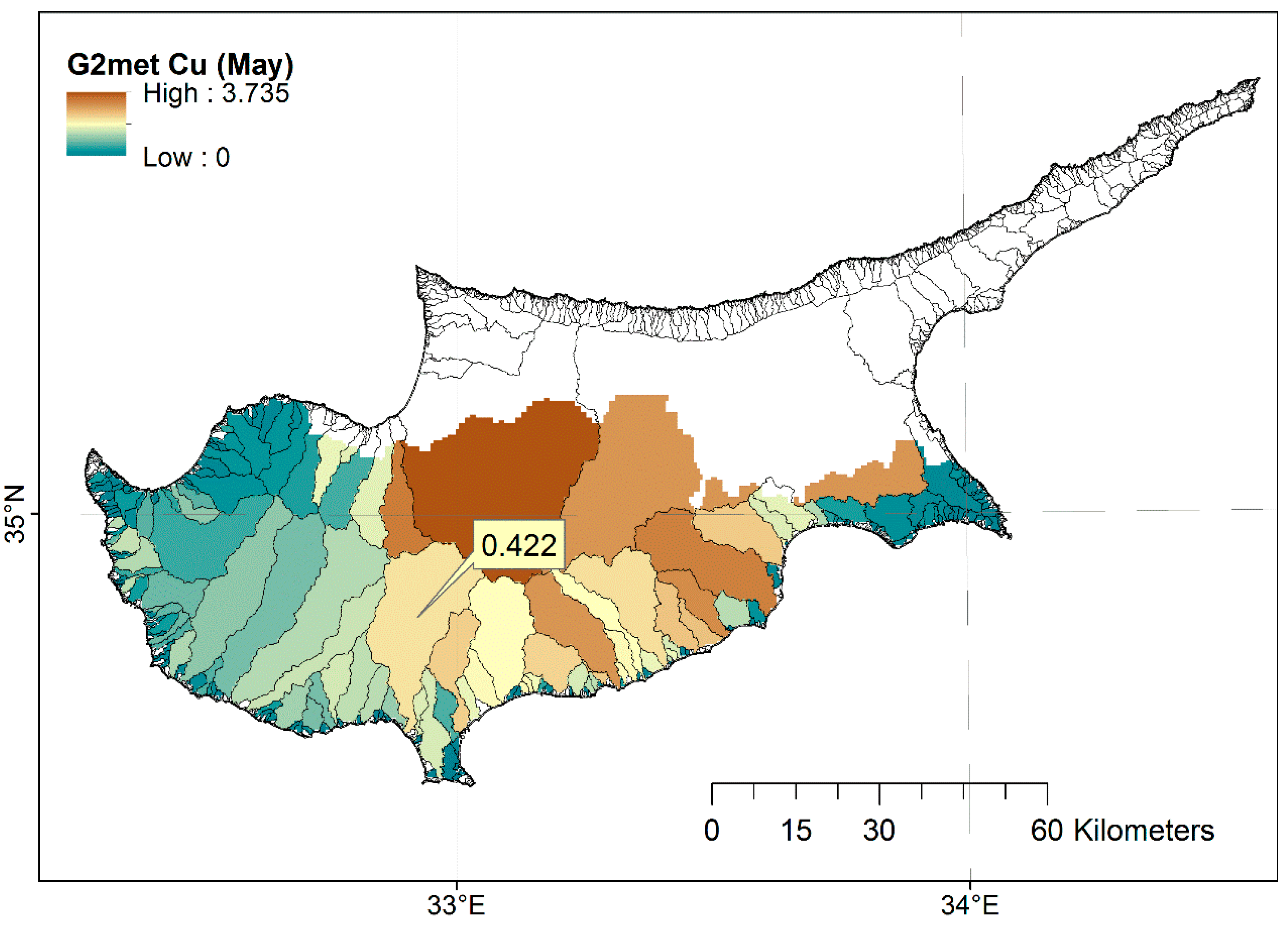
3.5. G2met Risk Maps and Statistics

Using Equation (2), twelve G2met layers and another one for the annual risk assessment were created per heavy metal. In addition to that, another twelve layers (i.e., one per month) plus an annual layer were created for the total risk in the study area. As a result, 117 risk layers at 500-m cell size were produced (Figure 6). This big set of layers allows for a detailed monitoring of contamination risk associated with heavy metals in the study area in the spatiotemporal domain (Table 3).

Due to the linear character of the main G2met equation, the monthly distribution of the total risk by G2met follows the same temporal trend as that of erosion. Also, the two layers are overall spatially equivalent, as the mean ratio of normalized (with the mean) annual G2met total risk layer over the normalized (with the mean) Hakanson index layer, was found to be 0.98. Therefore, the main effect of incorporating erosion processes in the calculation of the G2met index (in comparison to the use of the Hakanson index alone) is the spatial redistribution of risk (Figure 7).

Figure 6. Annual G2met index map for the total risk (cell size: 500 m; value ranging: histogram equalization; mean value: 146.2).

Figure 6. Annual G2met index map for the total risk (cell size: 500 m; value ranging: histogram equalization; mean value: 146.2).

Table 3. Mean values of G2met layers per heavy metal and month (Hakanson values included for comparison).

Month	Cd	Cr	Cu	Ni	Pb	Zn	Hg	As	Total
January	3.437	0.228	0.610	0.632	0.920	0.130	3.873	0.873	10.707
February	1.751	0.103	0.256	0.284	0.498	0.058	1.622	0.397	4.971
March	1.012	0.055	0.143	0.150	0.283	0.032	0.853	0.220	2.752
April	0.962	0.048	0.134	0.142	0.230	0.027	0.792	0.212	2.549
May	3.852	0.289	0.880	0.885	0.760	0.142	4.778	1.094	12.657
June	3.526	0.239	0.730	0.747	0.769	0.126	4.739	0.917	11.796
July	4.306	0.318	0.989	1.008	0.864	0.158	7.839	1.156	16.641
August	1.740	0.112	0.405	0.423	0.374	0.068	3.206	0.425	6.730
September	2.846	0.217	0.529	0.589	0.723	0.115	3.234	0.802	9.058
October	7.607	0.622	1.700	1.774	1.780	0.316	10.700	2.207	26.709
November	8.027	0.617	1.708	1.762	1.830	0.323	10.426	2.250	26.947
December	6.342	0.404	1.069	1.101	1.619	0.229	6.568	1.634	18.968
Annual (total)	44.409	3.208	8.752	9.164	10.510	1.679	56.530	11.950	146.208
Hakanson	11.905	0.965	2.197	2.931	2.832	0.447	12.520	3.285	37.086

Table 3. Mean values of G2met layers per heavy metal and month (Hakanson values included for comparison).

Month	Cd	Cr	Cu	Ni	Pb	Zn	Hg	As	Total
January	3.437	0.228	0.610	0.632	0.920	0.130	3.873	0.873	10.707
February	1.751	0.103	0.256	0.284	0.498	0.058	1.622	0.397	4.971
March	1.012	0.055	0.143	0.150	0.283	0.032	0.853	0.220	2.752
April	0.962	0.048	0.134	0.142	0.230	0.027	0.792	0.212	2.549
May	3.852	0.289	0.880	0.885	0.760	0.142	4.778	1.094	12.657
June	3.526	0.239	0.730	0.747	0.769	0.126	4.739	0.917	11.796
July	4.306	0.318	0.989	1.008	0.864	0.158	7.839	1.156	16.641
August	1.740	0.112	0.405	0.423	0.374	0.068	3.206	0.425	6.730
September	2.846	0.217	0.529	0.589	0.723	0.115	3.234	0.802	9.058
October	7.607	0.622	1.700	1.774	1.780	0.316	10.700	2.207	26.709
November	8.027	0.617	1.708	1.762	1.830	0.323	10.426	2.250	26.947
December	6.342	0.404	1.069	1.101	1.619	0.229	6.568	1.634	18.968
Annual (total)	44.409	3.208	8.752	9.164	10.510	1.679	56.530	11.950	146.208
Hakanson	11.905	0.965	2.197	2.931	2.832	0.447	12.520	3.285	37.086

Figure 7. The layer of ratio between normalized (with the mean) layers of annual G2met total risk and Hakanson index (cell size: 500 m; value ranging: histogram equalization; mean value = 0.98).

Figure 7. The layer of ratio between normalized (with the mean) layers of annual G2met total risk and Hakanson index (cell size: 500 m; value ranging: histogram equalization; mean value = 0.98).

A mean value per river basin was calculated from the produced G2met layers of monthly and annual risk levels, either for each heavy metal individually or for all heavy metals together. An exploration of the Hakanson and G2met layers per basin shows a dramatic effect of the erosion component of the G2met model on the mapping result, in comparison to the (static) Hakanson index alone. In an indicative comparison for the total risk using normalized risk values (range 0–1), many basins appearing to have low risks with the Hakanson index, show highly risky with the G2met index; and the inverse (Figure 8 and Figure 9).

Radical changes over months can be understood for every metal, as a result of the temporal component of the G2met model (i.e., the monthly step of the assessments). Indicatively, the risk maps of Cu for January and May, respectively, per river basin (mean values) exhibit very different spatial distribution of risk values per basin; e.g., there are basins which are classified in the high risk range in January, whereas in May the risk decreases substantially; and the inverse (see for example, Kouris basin) (Figure 10 and Figure 11).

Figure 8. Choropleth map of the Hakanson index for total risk per basin (value ranging: histogram equalization; mean value: 37.1; normalized mean value: 0.22).

Figure 8. Choropleth map of the Hakanson index for total risk per basin (value ranging: histogram equalization; mean value: 37.1; normalized mean value: 0.22).

Figure 9. Choropleth map of annual G2met index for total risk per basin (value ranging: histogram equalization; mean value: 142.8; normalized mean value: 0.30).

Figure 9. Choropleth map of annual G2met index for total risk per basin (value ranging: histogram equalization; mean value: 142.8; normalized mean value: 0.30).

Figure 10. Choropleth map of the mean G2met index values for Cu per basin in January (value ranging: histogram equalization; indicative example of Kouris basin, 1.156).

Figure 10. Choropleth map of the mean G2met index values for Cu per basin in January (value ranging: histogram equalization; indicative example of Kouris basin, 1.156).

Figure 11. Choropleth map of the mean G2met index values for Cu per basin in May (value ranging: histogram equalization; indicative example of Kouris basin, 0.422).

Figure 11. Choropleth map of the mean G2met index values for Cu per basin in May (value ranging: histogram equalization; indicative example of Kouris basin, 0.422).

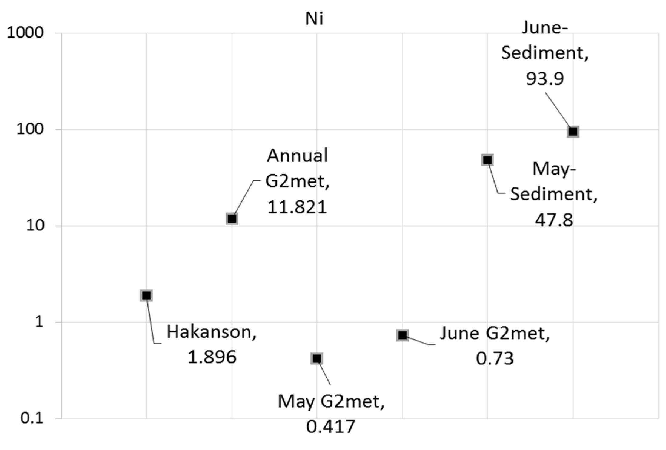
3.6. Evaluation Study

One of the largest reservoirs of Cyprus is the Kouris reservoir, located downstream of the Troodos Ophiolite complex and covering significant drinking water needs. The basin draining to Kouris reservoir covers an extent of about 304 km² (Figure 12). Covering a surface of about 1.95 km² on average, Kouris reservoir has a storage capacity of 115 Mm³ and the usable surface and groundwater capacity is 370 Mm³. Thus, Kouris reservoir stores the 31% of the usable water mass and is of high importance serving as a drinking water supply.

Figure 12. Located in the south part of Cyprus, Kouris reservoir was used for a risk assessment verification study.

Figure 12. Located in the south part of Cyprus, Kouris reservoir was used for a risk assessment verification study.

A sampling campaign took place in May 1012 and June 2014 to obtain sediment samples from four different locations in Kouris reservoir (depth range 48.3–77.9 m). The most abundant heavy metals were Cr, Ni, and Cu (Table 4).

The mean G2met index values for Ni, Cr, and Cu in Kouris basin were calculated and their temporal distribution (on a monthly basis) was graphed (Figure 13). From this graph, a large temporal fluctuation of risk for both metals can be detected, with October to December being distinctly the highest risk months, January, June, July, and September being moderate in risk, and the other months being at lower risk levels. These findings are in accordance with the relatively low concentration values indicated for this season of the year (May to June) in the sampled heavy metals of Kouris reservoir. (Note that Cr values appear lower than those of Ni and Cu due to the fact that Cr has been assigned a lower toxicity factor).

Table 4. Mean values in mg kg⁻¹ and standard deviation (SD) of heavy metals of sediment in Kouris reservoir (DL-Detection Level).

Element Name	Sediments Samples (n = 4) May 2012		Sediments Samples (n = 4) June 2014
	Mean	SD	Mean	SD
Ni	246.1	264.4	105.7	21
Cr	123.2	134.6	–	–
Cu	47.8	7.2	93.9	12.9
Zn	16.7	6.1	46.6	3.5
As	<DL	–	–	–
Cd	<DL	–	2.2	0.3
Hg	<DL	–	<DL	–
Pb	5.6	4.0	36.7	4.4

Table 4. Mean values in mg kg⁻¹ and standard deviation (SD) of heavy metals of sediment in Kouris reservoir (DL-Detection Level).

Element Name	Sediments Samples (n = 4) May 2012		Sediments Samples (n = 4) June 2014
	Mean	SD	Mean	SD
Ni	246.1	264.4	105.7	21
Cr	123.2	134.6	–	–
Cu	47.8	7.2	93.9	12.9
Zn	16.7	6.1	46.6	3.5
As	<DL	–	–	–
Cd	<DL	–	2.2	0.3
Hg	<DL	–	<DL	–
Pb	5.6	4.0	36.7	4.4

Figure 13. Monthly distribution of G2met index values for Ni, Cr, and Cu in Kouris reservoir.

Figure 13. Monthly distribution of G2met index values for Ni, Cr, and Cu in Kouris reservoir.

An indicative overview of the estimated risk values in Kouris basin in comparison to the measured concentration values in the sediment samples for Ni (in mg kg⁻¹) in the Kouris reservoir, is provided in Figure 14.

Figure 14. Indicative overview graph of estimated risk values (logarithmic scale) of Ni in the Kouris basin and Ni concentrations in sediments (in mg·kg⁻¹) in Kouris reservoir.

Figure 14. Indicative overview graph of estimated risk values (logarithmic scale) of Ni in the Kouris basin and Ni concentrations in sediments (in mg·kg⁻¹) in Kouris reservoir.

4. Conclusions and Outlook

In this research, a new risk index for surface water contamination by heavy metal concentrations in soils was developed. The new index, namely the G2met index, is by default spatiotemporal, in terms of producing standardized month-time step risk maps. Considering that the new index incorporates the Hakanson index (as a term in the main equation), future studies (using G2met) will be comparable to previous ones (using Hakanson).

An application of the new index in Cyprus showed that it is a useful tool for supporting analysis of ecosystems threatened by heavy metals. In water shortage areas, such as in Cyprus, construction of reservoirs is a common solution for water storage and management, even though the eroded sediment is trapped into their bed. Therefore, in these cases, special attention should be given in examining the potential of sediment to act as pollution source or sink. A preliminary (though limited) evaluation study of the G2met index for Ni, Cr, and Cu in Kouris basin showed that measured values were in accordance with the estimated ones. It seems that G2met is more realistic than previous attempts.

More extended and detailed experiments should be conducted in order to assist in elaboration of an extra factor in the G2met methodology, accounting for soil fraction in the sediment loads. As it is known, fine soil fraction facilitates adsorption and metal binding to iron and manganese oxides and to organic matter and experiences usually high metal concentrations.

References

1. Davies, O.A.; Abowei, J.F.N. Sediment quality of lower reaches of Okpoka Creek, Niger Delta, Nigeria. Eur. J. Sci. Res. 2009, 26, 437–442. [Google Scholar]
2. Adeyemo, O.K.; Adedokun, O.A.; Yusuf, R.K.; Adeleye, E.A. Seasonal changes in physicao-chemical parameters and nutrient load of river sediment in Ibadan city, Nigeria. Glob. NEST J. 2008, 10, 326–336. [Google Scholar]
3. Gong, Q.J.; Deng, J.; Xiang, Y.C. Calculating Pollution Indices by Heavy Metals in Ecological Geochemistry Assessment and a Case Study in Parks of Beijing. J. China Univ. Geosci. 2008, 19, 230–241. [Google Scholar]
4. Müller, G. Index of geoaccumuation in sediments of the Rhine River. Geosci. J. 1969, 2, 108–118. [Google Scholar]
5. Li, X.; Lee, S.; Wong, S.; Wong, S.C.; Shi, W.Z.; Thornton, I. The study of metal contamination in urban soils of Hongkong using a GIS-based approach. Environ. Pollut. 2004, 129, 113–124. [Google Scholar] [CrossRef] [PubMed]
6. Nikolaidis, C.; Zafiriadis, I.; Mathioudakis, V.; Constantinidis, T. Heavy Metal Pollution Associated with an Abandoned Lead–Zinc Mine in the Kirki Region. Bull. Environ. Contam. Toxicol. 2010, 85, 307–312. [Google Scholar] [CrossRef] [PubMed]
7. Wei, B.; Yang, L. A review of heavy metal contaminations in urban soils, urban road dusts and agricultural soils from China. Microchem. J. 2010, 94, 99–107. [Google Scholar] [CrossRef]
8. Li, Z.Y.; Ma, Z.W.; van der Kuijp, T.J.; Yuan, Z.W.; Huang, L. A review of soil heavy metal pollution from mines in China: Pollution and health risk assessment. Sci. Total Environ. 2014, 468, 843–853. [Google Scholar] [CrossRef] [PubMed]
9. Hakanson, L. An ecological risk index aquatic pollution control, a sedimentological approach. Water Res. 1980, 14, 975–1001. [Google Scholar] [CrossRef]
10. Pradhan, B.; Lee, S.; Buchroithner, M.F. Use of geospatial data and fuzzy algebraic operators to landslide-hazard mapping. Appl. Geomat. 2009, 1, 3–15. [Google Scholar] [CrossRef]
11. Brooks, N. Vulnerability, Risk and Adaptation: A Conceptual Framework. Available online: http://www.tyndall.ac.uk/sites/default/files/wp38.pdf (accessed on 30 May 2015).
12. Pediaditi, K.; Stanojevic, M.M.; Kouskouna, C.G.; Karydas, D.; Ziannis, G.; Boretos, N. A decision support system for assessing and managing environment risk cross borders. Earth Sci. Inform. 2011, 4, 107–115. [Google Scholar]
13. Pistocchi, R.; Pezzolesi, L.; Guerrini, F.; Vanucci, S.; Dell’aversano, C.; Fattorusso, E. A review on the effects of environmental conditions on growth and toxin production of Ostreopsis ovata. Toxicon 2011, 57, 421–428. [Google Scholar] [CrossRef] [PubMed]
14. Lahr, J.; Kooistra, L. Environmental risk mapping of pollutants: State of the art and communication aspects. Sci. Total Environ. 2010, 408, 3899–3907. [Google Scholar] [CrossRef] [PubMed]
15. Fraser, E.D.G.; Dougill, A.; Mabee, W.; Reed, M.S.; McAlpine, P. Bottom up and top down: Analysis of participatory processes for sustainability indicator identification as a pathway to community empowerment and sustainable environmental management. J. Environ. Manag. 2006, 78, 114–127. [Google Scholar] [CrossRef] [PubMed]
16. Besio, M.; Ramella, A.; Bobbe, A.; Colombo, A.; Olivieri, C.; Persano, M. Risk maps: Theoretical concepts and techniques. J. Hazard. Mater. 1998, 61, 299–304. [Google Scholar] [CrossRef]
17. Bartels, C.J.; van Beurden, A.U.C.J. Using geographic and cartographic principles for environmental assessment and risk mapping. J. Hazard. Mater. 1998, 61, 115–124. [Google Scholar] [CrossRef]
18. Karydas, C.G.; Sarakiotis, I.L.; Zalidis, G.C. Multi-scale risk assessment of stream pollution by wastewater of olive oil mills in Kolymvari, Crete. Earth Sci. Inform. 2014, 7, 47–58. [Google Scholar] [CrossRef]
19. Driesen, P.M. Erosion hazards and conservation needs as a function of land characteristics and land qualities. In Land Evaluation for Land-Use Planning and Conservation in Sloping Areas; ILRI: Wageningen, The Netherlands, 1986; pp. 32–39. [Google Scholar]
20. Aksoy, H.; Kavvas, M.L. A review of hillslope and watershed scale erosion and sediment transport models. Catena 2005, 64, 247–271. [Google Scholar] [CrossRef]
21. Olubunmi, F.E.; Olorunsola, O.E. Evaluation of the status of heavy metal pollution of sediment of agbabu bitumen deposit area, Nigeria. Eur. J. Sci. Res. 2010, 41, 373–382. [Google Scholar]
22. Karydas, C.G.; Zdruli, P.; Koci, S.; Sallaku, F. Month-step erosion risk monitoring of Ishmi-Erzeni watershed, Albania using the G2 model. Environ. Model. Assess. 2015, 4, 1–16. [Google Scholar]
23. Gavrilovic, Z. The use of empirical method (erosion potential method) for calculating sediment production and transportation in unstudied or torrential streams. In Proceeding of the International Conference on River Regime, Chichester, UK, 12 August 1988; pp. 411–422.
24. US Environmental Protection Agency (EPA). Available online: http://water.epa.gov/polwaste/nps/whatis.cfm (accessed on 30 May 2015).
25. Panagos, P.; Meusburger, K.; Ballabio, C.; Borrelli, P.; Alewell, C. Soil erodibility in Europe: A high-resolution dataset based on LUCAS. Sci. Total. Environ. 2014, 479, 189–200. [Google Scholar] [CrossRef] [PubMed] [Green Version]
26. Westrich, B.; Kern, U. Mobility of Contaminants in the Sediments of Lock-Regulated Rivers-Field Experiments in the Lock Reservoir Lauffen, Modeling and Estimation of the Remobilisation Risk of Older Sediment Deposits; University of Stuttgart: Stuttgart, Germany, 1996. [Google Scholar]
27. Dos Santos, S.N.; Alleoni, L.R. Reference values for heavy metals in soils of the Brazilian agricultural frontier in Southwestern Amazonia. Environ. Monit. Assess. 2013, 18, 5737–5748. [Google Scholar] [CrossRef] [PubMed]
28. Cohen, D.R.; Rutherford, N.F.; Morisseau, E.; Zissimos, A.M. Geochemical patterns in the soils of Cyprus. Sci. Total Environ. 2012, 420, 250–262. [Google Scholar] [CrossRef] [PubMed]
29. Westrich, B.; Forstrner, U. Sediment Dynamics and Pollutant Mobility in Rivers: An Interdisciplinary Approach; Springer: Berlin, Germany, 2007. [Google Scholar]
30. Oliveira, S.M.B.; Pessenda, L.C.R.; Gouveia, S.E.M.; Favaro, D.I.T. Heavy metal concentrations in soils from a remote oceanic island, Fernando de Noronha, Brazil. An. Acad. Bras. Cienc. 2011, 83, 1193–1206. [Google Scholar] [CrossRef] [Green Version]
31. Gawlik, B.M.; Bidoglio, G. Background Values in European Soils and Sewage Sludges, PART III Conclusions, Comments and Recommendations. Available online: http://eusoils.jrc.ec. europa.eu/ESDB_Archive/eusoils_docs/other/eur22265_3.pdf (accessed on 30 May 2015).
32. Karydas, C.G.; Panagos, P.; Gitas, I.Z. A classification of water erosion models according to their geospatial characteristics. Int. J. Digit. Earth 2012, 7, 229–250. [Google Scholar] [CrossRef]
33. Panagos, P.; van Liedekerke, M.; Jones, A.; Montanarella, L. European soil data centre: Response to European policy support and public data requirements. Land Use Polic. 2012, 29, 329–338. [Google Scholar] [CrossRef]
34. Panagos, P.; Ballabio, C.; Borrelli, P.; Meusburger, K.; Klik, A.; Rousseva, S.; Tadić, M.P.; Michaelides, S.; Hrabalíková, M.; Olsen, P.; et al. Rainfall erosivity in Europe. Sci. Total Environ. 2015, 511, 801–814. [Google Scholar] [CrossRef] [PubMed]
35. Meusburger, K.; Steel, A.; Panagos, P.; Montanarella, L.; Alewell, C. Spatial and temporal variability of rainfall erosivity factor for Switzerland. Hydrol. Earth Syst. Sci. 2012, 16, 167–177. [Google Scholar] [CrossRef] [Green Version]
36. Hijmans, R.J.; Cameron, S.E.; Parra, J.L.; Jones, P.G.; Jarvis, A. Very high resolution interpolated climate surfaces for global land areas. Int. J. Clim. 2015, 25, 1965–1978. [Google Scholar] [CrossRef]
37. Hastie, T.J.; Tibshirani, R.J. Generalized Additive Models; CRC Press: Boca Raton, FL, USA, 1990. [Google Scholar]
38. VITO client ftp portal. Available online: catftp.vgt.vito.be (accessed on 30 May 2015).
39. Verhoef, W. Earth observation modeling based on layer scattering matrices. Remote Sens. Environ. 1985, 17, 165–178. [Google Scholar] [CrossRef]
40. Panagos, P.; Karydas, C.; Ballabio, C.; Gitas, I. Seasonal monitoring of soil erosion at regional scale: an application of the G2 model in Crete focusing on agricultural land uses. Int. J. Appl. Earth Obs. Geoinform. 2014, 27, 147–155. [Google Scholar] [CrossRef]
41. Renard, K.G.; Foster, G.R.; Weessies, G.A.; McCool, D.K. Predicting Soil Erosion by Water: A Guide to Conservation plaNning with the REVISED Universal Soil Loss Equation (RUSLE); United States Department of Agriculture: Washington, DC, USA, 1997.
42. Moore, I. D.; Burch, G.J. Physical basis of the lengthslope factor in the universal soil loss equation. Soil Sci. Soc. Am. J. 1986, 50, 1294–1298. [Google Scholar] [CrossRef]
43. United States Geological Survey (USGS) portal. Available on line: http://earthexplorer.usgs.gov/ (accessed on 30 May 2015).
44. Alexakis, D.D.; Hadjimitsis, D.G.; Agapiou, A. Integrated use of remote sensing, GIS and precipitation data for the assessment of soil erosion rate in the catchment area of “Yialias” in Cyprus. Atmos. Res. 2013, 131, 108–124. [Google Scholar] [CrossRef]
45. O’Callaghan, J.F.; Mark, D.M. The extraction of drainage networks from digital elevation data. Comput. Vis. Graph. Image Process. 1984, 28, 328–344. [Google Scholar]