3.1. Characteristics of the Flood Events
Table 3 summarizes the general characteristics of the rainfall, runoff, suspended sediment, and antecedent conditions associated with the observed floods and variables as analyzed by statistical analysis.
The maximum amount of precipitation for a single event was 72.7 mm (during the event on 3 June 2004); most of the events were relatively small in magnitude. Only 10 events (34%) were greater than the average rainfall value (27.8 mm), whereas the remaining events were below the average. The mean intensity varied from 0.63 to 10.45 mm·h−1, and eight events were greater than the mean value (2.74 mm·h−1). The maximum 30 min intensity ranged from 1.3 to 30 mm; 24% exceeded 10 mm during the 30 min interval, and eight of the events were greater than the average value (6.89 mm). The antecedent rainfall values varied considerably, ranging from 0 to 24.6 mm, 0 to 69.2 mm, and 0.1 to 89.0 mm of precipitation during the 1-, 5-, and 10-day previous periods, respectively.
Figure 3.
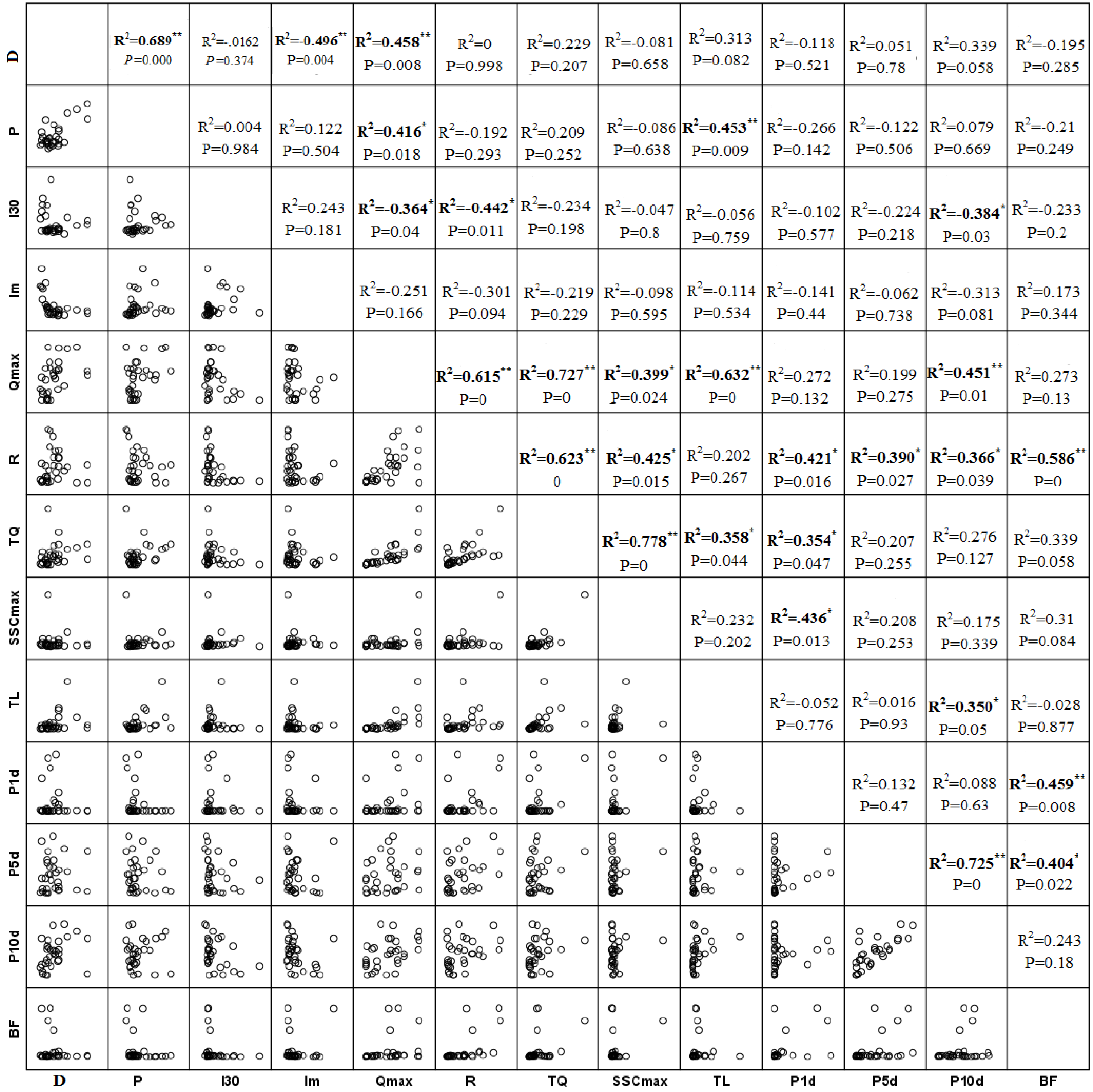
Bivariate scatter plot matrix of selected event characteristics. Note: ** means very significant levels (p < 0.01), and * means significant levels (p < 0.05).
Figure 3.
Bivariate scatter plot matrix of selected event characteristics. Note: ** means very significant levels (p < 0.01), and * means significant levels (p < 0.05).
The runoff generated by rainfall varied between 3674 and 309,618 m
3, with a mean value of 100,459 m
3. Peak discharge oscillated between 0.05 and 5.59 m
3·s
−1. The peak was greater than the mean value (2.20 m
3·s
−1) during 16 floods (55% of the total sample). The baseflow level fluctuated from 0.006 to 0.857 m
3·s
−1. The maximum flood sediment concentrations varied from 130 to 18,200 g·m
−3; with a mean concentration of 1740 g·m
−3. The total suspended sediment load carried by 15 floods exceeded 167 t (representing a specific suspended sediment yield of 10·t·km
−2). The maximum yield during a single flood occurred on 4 June 2004 and reached 412,651 kg. This yield was generated by 72.7 mm of precipitation, which created a flood peak discharge of 5.44 m
3·s
−1. These values illustrate the degree of geomorphic activity of the system and confirm the high sediment contribution and transport capacity of the channels in the Wangjiaqiao watershed, which are largely related to the availability of fine materials in the TGA areas and the accumulation of these materials along the main channel [
15].
We generated a Pearson correlation matrix (
Figure 3). The linear correlation coefficients among rainfall-, runoff-discharge-, sediment-, and antecedent condition-related variables are described in detail. Peak flow (
Qmax) was significantly correlated with
R,
TQ,
SSCmax,
TL, and
P10D. The strongest correlation was between precipitation (
TQ) and runoff (
Qmax). Runoff was significantly correlated with
TQ,
SSCmax,
P1D,
P5D,
P10D, and
BF. The results confirmed that many variables were co-linear.
3.3. Results of PLSR Analysis
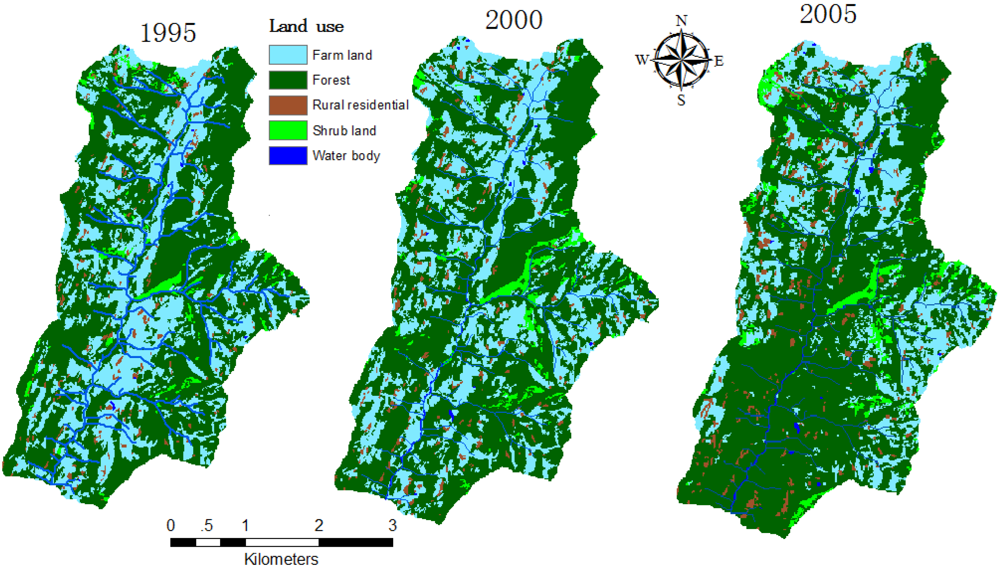
Many studies have demonstrated that land use type can change runoff and sediment yield [
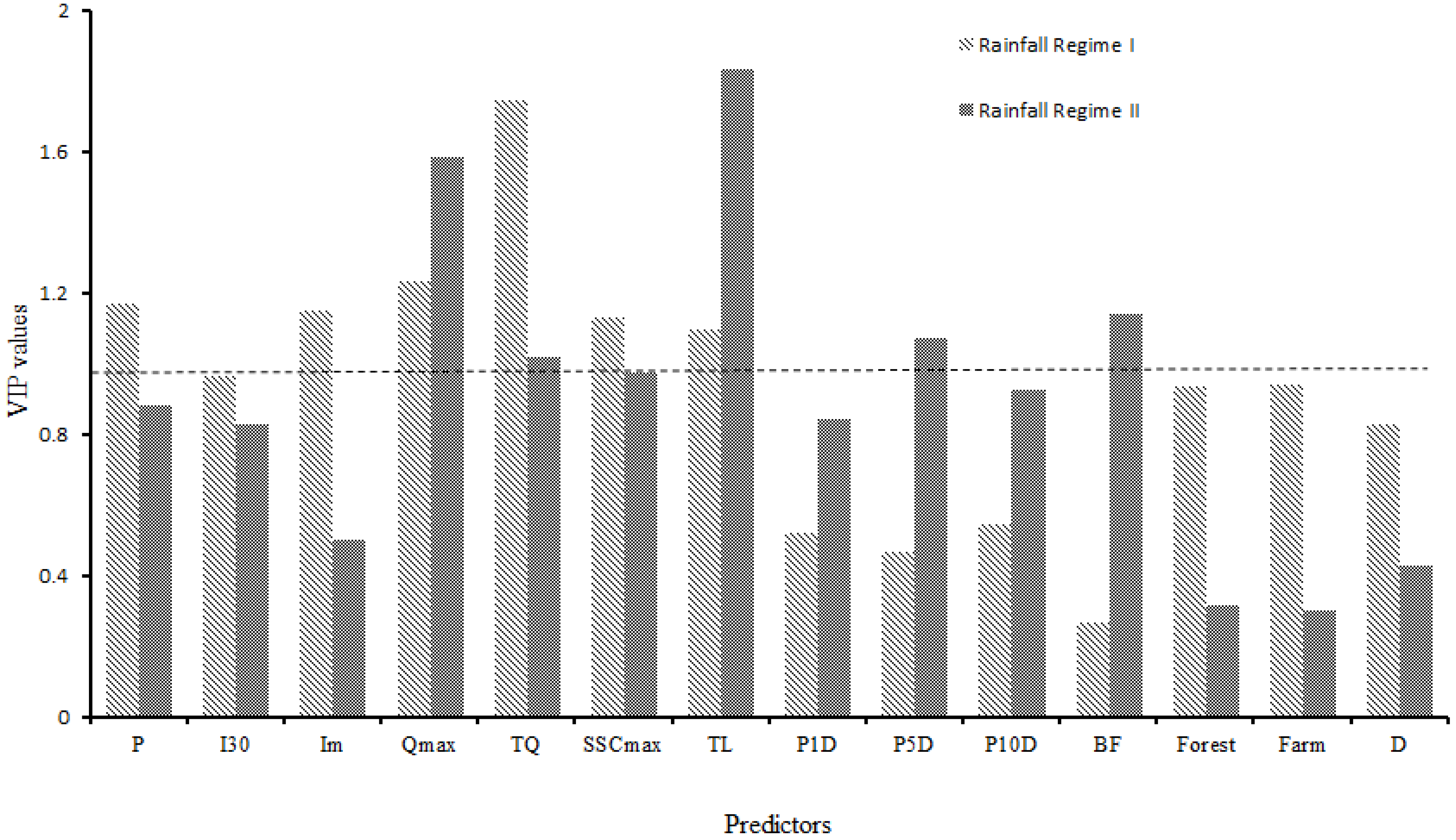
29]; thus, the percentages of forest and farmland during the study years were included in the PLSR models. In a PLSR model, the importance of a predictor for both the independent and dependent variables is given by the variable importance for the projection (VIP) [
10,
12]. Terms with large VIP values are the most relevant for explaining the dependent variable. To overcome the problem of over-fitting, the appropriate number of components of each PLSR model was determined by cross-validation to achieve an optimal balance between the explained variation in the response (R
2) and the predictive ability of the model (goodness of prediction: Q
2) [
10].
Table 5 provides a summary of the four PLSR models constructed separately for the runoff and sediment yield of the two rainfall regimes.
Table 5.
Summaries of the partial least squares regression (PLSR) models.
Table 5.
Summaries of the partial least squares regression (PLSR) models.
| Rainfall Regime | Response Variable Y | R2 | Q2 | Component | % of Explained Variability in Y | Cumulative Explained Variability in Y (%) | RMSECV a (m3 or kg) | Q2cum |
|---|
| Rainfall Regime I | R | 0.99 | 0.85 | 1 | 71.6 | 71.6 | 51,977 | 0.564 |
| 2 | 22.5 | 94.1 | 25,035 | 0.761 |
| 3 | 2.7 | 96.8 | 19,507 | 0.737 |
| 4 | 2.0 | 98.8 | 12,801 | 0.803 |
| 5 | 0.7 | 99.5 | 8862 | 0.852 |
| 6 | 0 | 99.5 | 9265 | 0.837 |
| TL | 0.97 | 0.62 | 1 | 80.6 | 80.6 | 52,181 | 0.570 |
| 2 | 16.2 | 96.8 | 24,088 | 0.624 |
| 3 | 1.9 | 98.7 | 16,500 | 0.587 |
| 4 | 0.5 | 99.2 | 13,434 | 0.546 |
| Rainfall Regime II | R | 0.90 | 0.65 | 1 | 69.6 | 69.6 | 41,776 | 0.444 |
| 2 | 20.1 | 89.7 | 25,167 | 0.646 |
| 3 | 3.3 | 93.0 | 21,477 | 0.610 |
| TL | 0.86 | 0.66 | 1 | 80.6 | 66.6 | 11,427 | 0.503 |
| 2 | 4.3 | 88.6 | 6912 | 0.656 |
| 3 | 1.4 | 92.2 | 5933 | 0.637 |
For the runoff model of Rainfall Regime I, the prediction error decreased with an increasing number of components, and the minimum RMSECV and maximum
Q2 were obtained with five components. An additional increase in the number of components generated a higher prediction error, suggesting that the other components were not strongly correlated with the residuals of the predicted variable [
12]. The first component explained 71.6% of the variance in the dataset in terms of the changes in runoff (
Table 5). The addition of the second through fifth components to the models cumulatively explained 99.5% of the total variance. For the
TL model of heavy rainfall, the maximum
Q2 was obtained with two components. The first component explained 80.6% of the variance in the dataset in terms of the changes in
TL. The second component explained 16.2% of the variance. These two components explained 96.8% of the total variance. Further addition of components to the PLSR models did not substantially increase the percentage of the variance explained (
Table 5). The PLSR weights could be used to describe the quantitative relationship between the predictors and results because they are linear combinations of the original variables that defined the scores [
28].
For the runoff model of moderate rainfall, the optimum model had two components, with a maximum Q2 of 0.646. The model explained 89.7% of the total variance, with 69.6% of the variance explained by the first component. The optimum model for the TL of moderate rainfall also contained two components. Those two components explained 88.6% of the total variance. The maximum Q2 was 0.656.
The first component of the runoff model for heavy rainfall (
Table 6) was dominated by
P,
Im,
Qmax,
TQ,
SSCmax, and
TL, whereas the second component was dominated by
Qmax and
TQ. The third, fourth, and fifth components were dominated by many variables, mainly on the negative side. A more convenient and comprehensive expression of the relative importance of the predictors was obtained by exploring their VIP values [
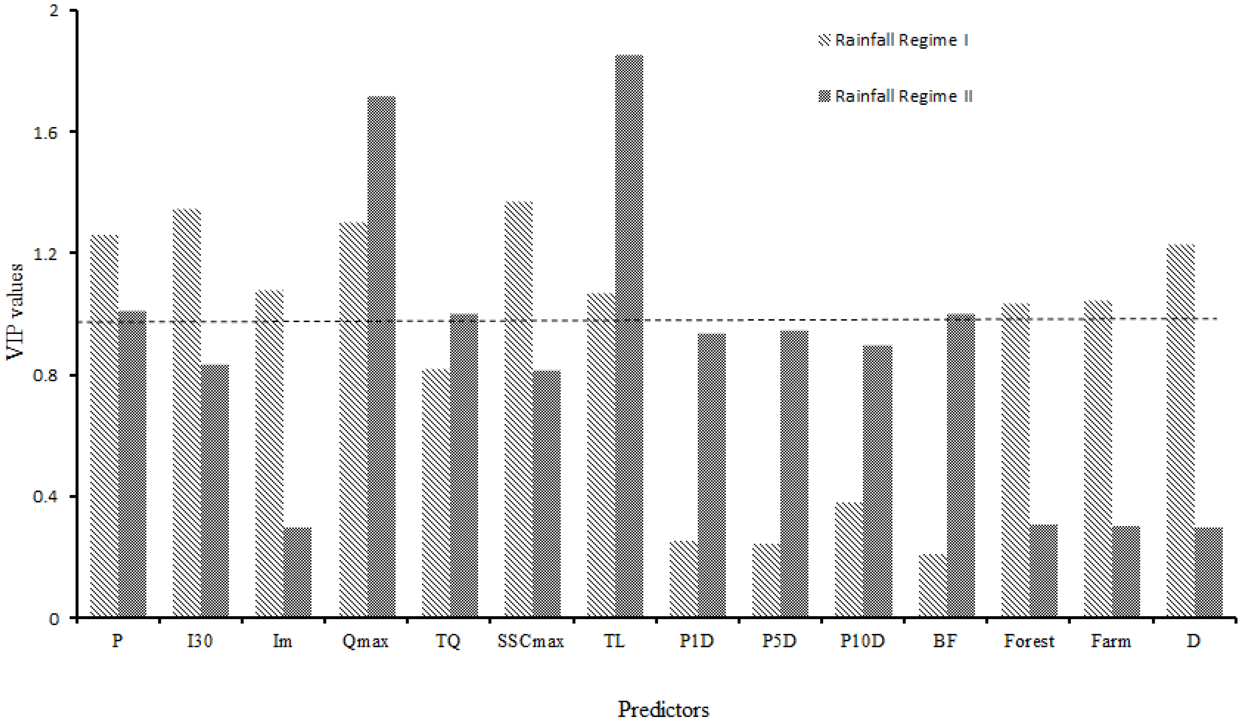
12]. For runoff in Rainfall Regime I, higher VIP values were obtained for changes in
TQ,
Qmax,
P,
Im,
SSCmax, and
TL (VIP > 1), followed by the percentage of forest and farmland (0.936 and 0.941) (
Figure 4). Predictors with VIP values below one are considered of minor predictive importance. For runoff in Rainfall Regime II, a higher VIP value was obtained for changes in
TL,
Qmax,
BF,
P5D, and
TQ. Compared with Rainfall Regime I, runoff in Rainfall Regime II was more likely to be affected by antecedent conditions, such as
BF and
P5D.
Table 6.
PLSR for runoff a.
Table 6.
PLSR for runoff a.
| Predictors | R of Rainfall Regime I | R of Rainfall Regime II |
|---|
| RCs b | W* (1) | W* (2) | W* (3) | W* (4) | W* (5) | RCs | W* (1) | W* (2) |
|---|
| P | −0.023 | 0.357 | −0.038 | −0.295 | −0.346 | −0.137 | 0.206 | 0.102 | 0.496 |
| I30 | −0.187 | 0.172 | −0.397 | −0.124 | −0.300 | −0.17 | −0.114 | −0.251 | −0.040 |
| Im | 0.005 | 0.344 | 0.161 | −0.469 | −0.486 | 0.025 | 0.110 | 0.036 | 0.289 |
| Qmax | 0.288 | 0.365 | 0.305 | 0.293 | −0.031 | −0.188 | 0.279 | 0.478 | 0.263 |
| TQ | 0.538 | 0.446 | 0.693 | 0.294 | 0.182 | 0.192 | 0.018 | 0.251 | −0.251 |
| SSCmax | 0.079 | 0.339 | −0.098 | −0.031 | 0.022 | 0.025 | −0.107 | 0.118 | −0.465 |
| TL | 0.195 | 0.334 | −0.024 | 0.278 | 0.212 | −0.074 | 0.388 | 0.523 | 0.536 |
| P1D | 0.024 | −0.129 | −0.164 | 0.175 | 0.194 | 0.731 | −0.053 | 0.147 | −0.339 |
| P5D | −0.193 | −0.011 | 0.103 | −0.620 | −0.325 | −0.499 | 0.151 | 0.325 | 0.061 |
| P10D | 0.326 | 0.099 | 0.138 | 0.218 | 0.927 | 0.414 | 0.063 | 0.258 | −0.122 |
| BF | 0.007 | −0.011 | 0.136 | 0.004 | −0.081 | −0.347 | 0.167 | 0.346 | 0.086 |
| Forest | 0.144 | 0.260 | −0.150 | 0.063 | 0.394 | 0.382 | −0.059 | −0.095 | −0.064 |
| Farm | −0.133 | −0.26 | 0.160 | −0.054 | −0.375 | −0.357 | 0.053 | 0.091 | −0.064 |
| D | −0.279 | 0.061 | −0.431 | −0.111 | −0.303 | −0.644 | 0.081 | 0.128 | 0.088 |
For the
TL model of Rainfall Regime I, higher VIP values were obtained for changes in
P,
I30,
Im,
Qmax,
SSCmax,
R, percentage of forest and farmland, and
D (see
Figure 5). Thus, all variables have important effects on
TL with the exception of antecedent conditions and
TQ. For the
TL model of Rainfall Regime II, high VIP values were obtained for
P,
Qmax,
TQ,
R, and
BF.
Table 7 indicates that
Qmax was important in the first and second components of Rainfall Regimes I and II, whereas
P5D and
P10D had only minor effects on
TL for either rainfall regime.
Figure 4.
VIP values of each predictor for PLSR of runoff.
Figure 4.
VIP values of each predictor for PLSR of runoff.
Figure 5.
VIP values of each predictor for PLSR of sediment load.
Figure 5.
VIP values of each predictor for PLSR of sediment load.
Table 7.
PLSR for sediment load.
Table 7.
PLSR for sediment load.
| Predictors | TL of Rainfall Regime I | TL of Rainfall Regime II |
|---|
| RCs a | W* (1) | W* (2) | RCs | W* (1) | W* (2) |
|---|
| P | 0.086 | 0.355 | −0.133 | 0.244 | 0.112 | 0.547 |
| I30 | 0.266 | 0.367 | 0.383 | −0.131 | −0.259 | −0.082 |
| Im | −0.116 | 0.200 | −0.559 | 0.052 | −0.014 | 0.156 |
| Qmax | 0.258 | 0.355 | 0.373 | 0.344 | 0.516 | 0.388 |
| TQ | 0.036 | 0.225 | −0.141 | 0.084 | 0.304 | −0.094 |
| SSCmax | 0.175 | 0.396 | 0.084 | 0.031 | 0.216 | −0.148 |
| R | 0.093 | 0.305 | −0.058 | 0.411 | 0.532 | 0.553 |
| P1D | −0.016 | −0.037 | 0.033 | −0.098 | 0.130 | −0.406 |
| P5D | −0.050 | −0.067 | −0.074 | 0.092 | 0.281 | −0.048 |
| P10D | 0.091 | 0.093 | 0.167 | −0.004 | 0.212 | −0.237 |
| BF | 0.021 | −0.042 | 0.106 | −0.008 | 0.233 | −0.272 |
| Forest | 0.048 | 0.285 | −0.170 | −0.052 | −0.097 | −0.039 |
| Farm | −0.056 | 0.291 | 0.152 | 0.048 | 0.094 | 0.031 |
| D | 0.292 | 0.296 | 0.536 | 0.083 | 0.134 | 0.182 |


