1. Introduction
Catastrophic flooding in the Sahelian part of the Niger basin has become an increasing threat during the last decades, leading to more than ten million people affected since the year 2000 [
1]. Tarhule
et al. (2005) [
2] were some of the first to bring the topic into academic research, referring to it as the “other Sahelian hazard”. Aich
et al. (2014) [
1] recently published a comprehensive overview of flooding characteristics within the entire Niger basin, including a review of existing literature and damage statistics from different sources. They found that the Sahelian part of the Niger basin was particularly affected by catastrophic floods, with an almost exponential increase in people affected over the last decades. They also showed that the increasing flood risk was related to the extreme population growth, the increasing vulnerability of the population, and an increase in flood magnitude.
However, the reason for the increase in flood magnitude in the Sahel is still not fully understood. Descroix
et al. (2012) [
3] stated that climate is not the cause of the phenomenon, since the increasing discharges are accompanied by decreasing rainfall rates. This inconsistency is called “the Sahel Paradox” (SP) and is described in detail in Descroix
et al. 2013 [
4]. Based on their statistical analysis and field observations on infiltration, they argued that the effect of land use and land cover change (LULC), from the local to the meso-scale, caused the increased discharge in the region. The main processes were land clearing and the transformation of savannah into pasture, agricultural land or degraded savannah. This led to soil crusting and a decrease in infiltrability, which subsequently led to an increase in flood magnitude during the heavy rains of the Sahelian rainy season.
In contrast to their study, Aich
et al. (2014) [
1] identified climatic changes and a return to wet conditions as the major driver of increasing flood magnitudes in the Niger basin, including the Sahelian region. Aich
et al. (2014) [
1] used a data-based attribution approach and compared time series of maximum annual discharge (AMAX) with precipitation time series, as well as time series of flashiness of discharge, as a proxy for LULC. They showed that even though the LULC caused an increase in flashiness since at least the 1960s, the AMAX decreased until the 1980s and they concluded that LULC could not be the major driver of the increased flood regime in the Sahel. In addition, they demonstrated that the SP only existed during the 1970s and 1980s, after which the trends of precipitation and discharge again correlated.
This study intends to contribute to the discussion on the reasons for the increasing flood risk in the Sahelian part of the Niger basin. The specific research question is, to which share LULC and/or climatic changes cause the increase of river flooding in the area. To this end, a simulation-based attribution approach proposed by Merz
et al. (2012) [
5] is used. Merz
et al. (2012) [
5] introduced a hypothesis testing framework for attributing changes of flood regime, which is based on testing the consistency or inconsistency of plausible drivers with the observed flood trend and providing a confidence level for the attribution. They distinguished between a data-based and a simulation-based attribution approach. The data-based attribution compares flood time series or their statistics with those of the assumed driver, for example, by evaluating the correlation between the time series of the potential cause and effect variables. It is common and widely used in the literature (e.g., [
1,
6,
7,
8,
9,
10,
11]). The simulation-based approach has been used in several studies with conceptual rainfall-runoff models [
12,
13,
14,
15,
16]. Process-based hydrological models have not been widely used for attribution approaches. There are studies, which distinguish climate change and LULC impacts on historical trends in flood magnitude, but not systematically and within one modeling approach (e.g., [
17]). To the best of our knowledge, the only study published which follows the protocol of Merz
et al. (2012) [
5] is that by Hundecha and Merz (2012) [
18]. Hundecha and Merz (2012) [
18] drove a hydrological model with a large number of stationary and non-stationary climate time series in order to study whether the observed flood trend was climate driven.
In this study, we analyze the effects of LULC on the flood trend using the process-based based ecohydrological model SWIM (Soil and Water Integrated Model) with integrated dynamic land use change. The ecohydrological model is applied to simulate flood discharges for the time period 1950–2009 with two different settings. The discharge is simulated with static land cover as of 1950 in order to show how the discharge would have developed over the last 60 years if there had not been any LULC. The second/control run implicitly includes past LULC. We hypothesize that the comparison of the modelled discharge of these two scenarios will give some initial quantitative insights into the relative share of LULC and climatic changes on changes in the Sahel flood regimes.
There is an ongoing debate over whether the observed “return to wet conditions” in West Africa itself can be attributed to global climate change or is still within the boundaries of natural climatic variability [
19,
20,
21]; without taking sides, we refer to the recent changes of the precipitation patterns as “climatic” changes.
Since this study is the first to attribute LULC to flood trends via a process-based hydrological model following the proposed protocol of Merz
et al. (2012) [
5], it might additionally shed first light on the requirements of data quality/availability and the efficiency of the hydrological model in order to achieve robust attribution statements.
2. Materials and Methods
2.1. Regional Setting
The Sahelian part of the Niger River is located downstream of Diré in Mali and extends to around Niamey in the state of Niger (
Figure 1). This part of the Niger basin until Niamey covers around 297,400 km
2. Its landscape is characterized by plateaus and smooth valleys with long slopes. The climate is semi-arid, with annual precipitation ranging from 267 mm in Ansongo to 540 mm in Niamey. The potential evapotranspiration in the area is 3500 mm per year [
3]. The typically convective rainfalls occur within the rainy season between June and October. The vegetation in the region and its changes since the 1950s are described in detail in Descroix
et al. (2012) [
3]. The original bushy and woody savannah types have been replaced almost completely by crop fields, pasture and a patchwork of woody savannah vegetation called Tiger Bush. The northern part, in which the Sirba catchment is located, is too dry for effective rain fed agriculture and was therefore turned mainly into extensively or intensively used pastoral land (
Figure 2 and
Figure 3). In contrast, the southern part in which the Sirba catchment is located has mainly been converted into cropland.
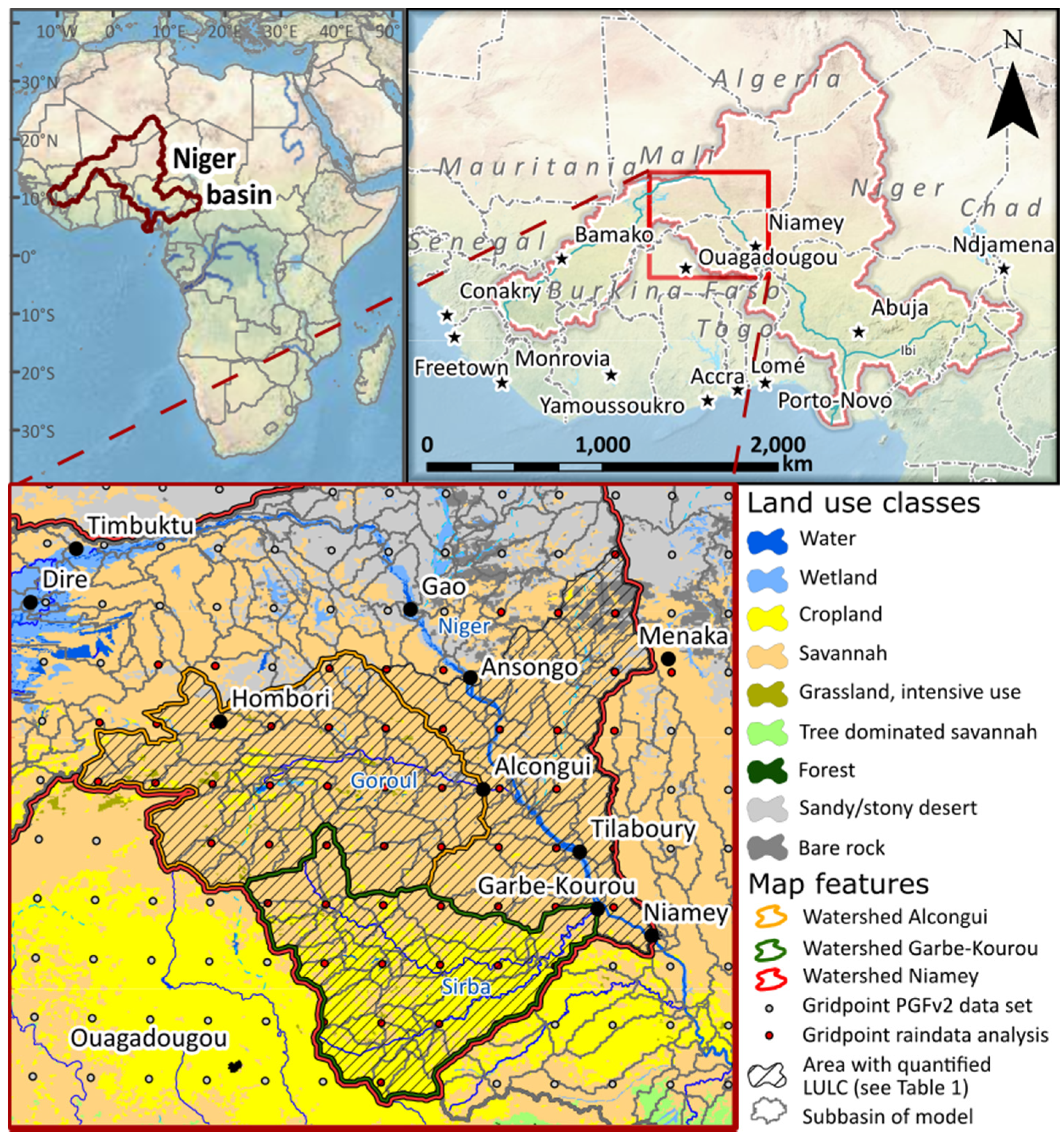
Figure 1.
Map of the research area in West Africa including land use classes used in the model as base map in the year 2000. The orange, green, and red outlines mark the watershed of the gauging stations Alcongui (Goroul River), Garbe-Kourou (Sirba River) and the watershed of Niamey (Niger River). The grey dots show the grid of the PGFv2 climate reanalysis data set. The red dots show the grid of the climate data used for the analysis. The hatched area marks the region which is used for the quantification of land use and land cover changes.
Most of the discharge in the Sahelian part of the Niger originates in its upstream regions within the Guinean highlands. The Inner Niger Delta, a large wetland, limits the Upper Niger basin. The wetland smooths the river flow and protracts the peak. The outlet of the delta is close to Diré, and the flood, generated in the Guinean highlands, occurs between November and January. This flood, referred to as the “Guinean Flood”, passes through Niamey between December and the beginning of March [
1]. Transmission losses are high between Diré and Niamey, resulting in higher annual discharge at Diré compared to Niamey. Little additional runoff is generated locally in the Sahelian part [
22]. This locally generated discharge comes mainly from the plateaus of the right-bank subbasins and results in another flood peak in the Sahelian Niger, previous to the Guinean Flood. This first peak occurs during the rainy season (July–November) and is called the “Red Flood” due to the red color of the sedimentary load of the local iron oxide rich soils. The two main tributaries are the Goroul (44,900 km
2) and Sirba Rivers (38,750 km
2), which are analyzed in this study (gauging stations Alcongui and Garbe-Kourou). Both are intermittent rivers, and the annual peaks vary substantially, with values between 35 and 300 m
3/s for Alcongui and 20 and 460 m
3/s for Garbe-Kourou (1950–2009). The vast subbasins to the East reach up into the central Sahara and contribute only a minor amount of inflow, and local tributaries are endorheic most of the year. The Guinean and Red Floods can usually be clearly distinguished. The peak of the Guinean Flood is already smoothed due to the large watershed and the dynamics of the Inner Niger Delta, whereas the peak of the Red Flood is more jagged and flashy. However, in years where the Red Flood is very low, a separate peak cannot be distinguished. This happened regularly during the 1950s and 1970s but has occurred significantly less often since the 1980s [
1].
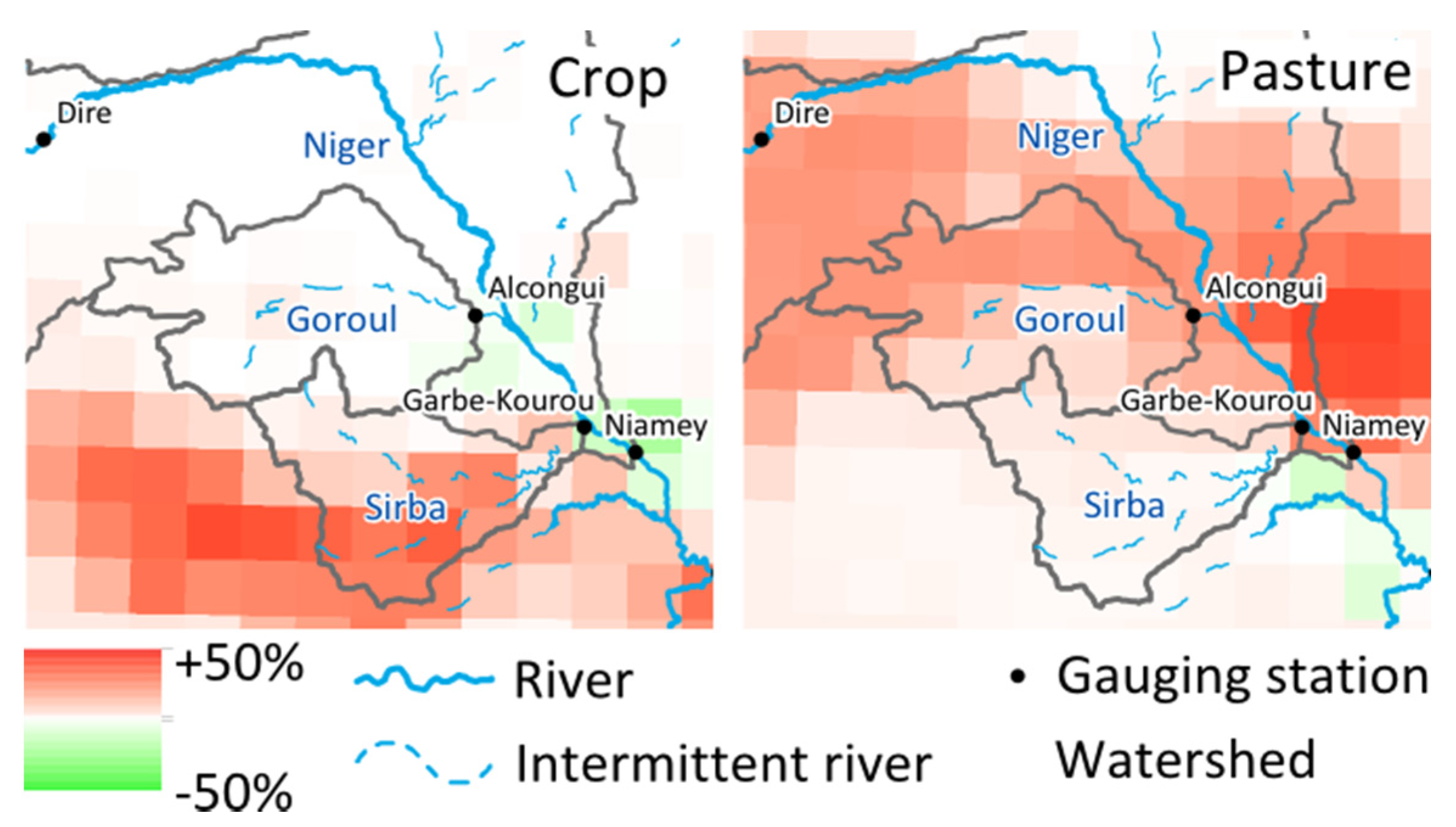
Figure 2.
Land use and land cover changes between 1950 and 2005 for crop and pasture after Hurtt
et al. (2011) [
23].
Figure 2.
Land use and land cover changes between 1950 and 2005 for crop and pasture after Hurtt
et al. (2011) [
23].
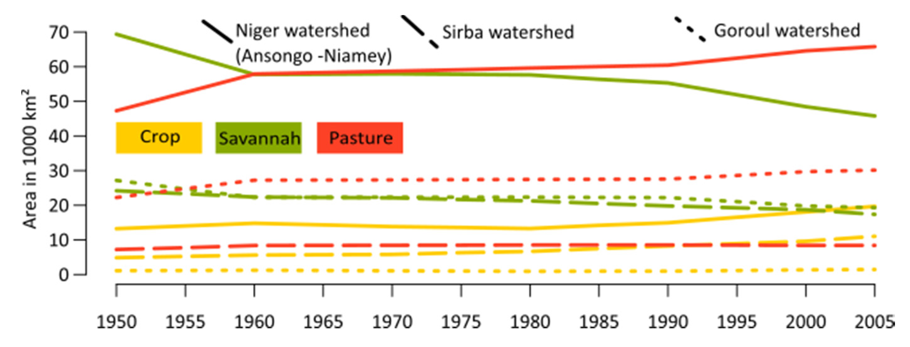
Figure 3.
Changes in the main land use classes of crop, savannah, and pasture from 1950 until 2005 for the watershed of the Niger River between Ansongo and Niamey, and the catchments of the Sirba and Goroul Rivers (see area in
Figure 1).
Figure 3.
Changes in the main land use classes of crop, savannah, and pasture from 1950 until 2005 for the watershed of the Niger River between Ansongo and Niamey, and the catchments of the Sirba and Goroul Rivers (see area in
Figure 1).
2.2. Ecohydrological Model and Model Set-Up
The ecohydrological model SWIM (Soil and Water Integrated Model) is a continuous-time (daily) and spatially semi-distributed model of intermediate complexity for river basins [
24]. SWIM was developed based on two models: Soil and Water Assessment Tool (SWAT) [
25] and MATSALU [
26], with the aim to provide a tool for climate and LULC impact assessment in meso-scale and large river basins. It integrates hydrological processes, vegetation growth, nutrient cycling, erosion and sediment transport at the river basin scale [
27]. The hydrological system of the model comprises four main segments: The soil surface, the root zone of the soil, the shallow aquifer, and the deep aquifer. On the soil surface, the surface runoff is estimated as a non-linear function of precipitation and a retention coefficient. It depends on soil water content, land use, and soil type (modified after the Soil Conservation Service curve number approach [
28]). The soil column is subdivided into several layers. In these layers, the water balance is calculated, including precipitation, surface runoff, evapotranspiration, subsurface runoff, and percolation. Hydrological processes represented in the shallow aquifer are groundwater recharge, capillary rise to the soil profile, lateral flow, and percolation to the deep aquifer. Potential evapotranspiration is calculated using the method of Turc-Ivanov [
29]. Actual evaporation from soil and transpiration by plants are simulated following the Ritchie concept [
30].
A simplified Environmental Policy Integrated Climate (EPIC) approach [
31] is integrated in the model for the simulation of arable crops and other general vegetation types (e.g., pasture, savannah, evergreen forest), using specific parameter values for each crop/vegetation type. The parameter settings of the newest version of the SWAT model are used for the aggregated vegetation types of the SWIM model [
32]. These parameter settings have been widely used in the African context for LULC studies (e.g., [
33,
34,
35,
36]). The effects of the vegetation on the hydrological processes include the cover-specific retention coefficient, impacting surface runoff and influencing the amount of transpiration. Transpiration is simulated as a function of potential evapotranspiration and leaf area index. A more detailed description of the representation of hydrological processes within SWIM is given in Huang
et al. (2013) [
27].
SWIM disaggregates a river basin into subbasins and hydrotopes. The subbasins are delineated on the basis of flow accumulation in a Digital Elevation Model. The hydrotopes are created by overlaying the subbasin map with maps of land use and soil. They represent the spatial units used to simulate all water flows and nutrient cycling in soil as well as vegetation growth based on the principle of similarity (
i.e., assuming that units within one subbasin that have the same land use and soil types behave similarly). The model was applied for impact studies in several basins in Africa and showed good efficiency for the whole Niger, the Blue Nile, the Limpopo and the Congo [
36,
37]. In addition, a multi-model intercomparison of hydrological models of Vetter
et al. (2015) has shown that SWIM is quite capable of simulating flow in the Niger basin [
38].
For this study, the model has been set up for the Sahelian part of the Niger River, from Diré in Mali to Niamey in the state of Niger. Since the model is only used for modeling river flows in the past, monitored discharges are routed into the model at the Diré gauge. The model includes 255 subbasins for the 297,000 km
2 area of the watershed. These subbasins are integrated to form three subcatchments which are the catchments Goroul (station Alcongui), Sirba (station Garbe-Kourou), and Niger (between the stations Diré and Niamey) (
Figure 1). These subcatchments were calibrated individually in order to fit the model as closely as possible to the regional conditions (see
Section 2.5.).
2.3. Dynamic Land Use Change Module
The newly developed land use change module (LUCM) for the SWIM model is used for the first time in this study. It changes the land classes at any frequency or given point in time, while keeping the instantaneous balance of water and other modelled fluxes constant during the change, for example soil water content (SWC). This means that the number and the areas of hydrotopes within a subbasin can change and new hydrotopes can appear or others disappear.
The land-use status at given points in time (see
Section 2.4.3) are read in by the LUCM (in this study every five years; Shorter frequencies up to a daily change are possible). The LUCM transforms the land classes and rearranges the hydrotopes on the basis of so-called stable units (SU). SU are areas within a subbasin and do not change their extent, like areas with uniform soil, for example. For these SU, fluxes like SWC remain constant during the change, even if the land class changes. Thereby, all given information on LULC on the subbasin level is used, and the transformation of the hydrotopes does not alter the balances of water or other relevant fluxes.
The following two examples shall illustrate the main processes when hydrotopes increase or decrease within a SU. If the shares of crop and pasture increase and the savannah deceases, the SWC of the old hydrotopes have to be newly distributed. The SWC of the savannah is reduced according to its areal share. The residual SWC is then added proportionally to crop and pasture, depending on their areal increase.
In another case, an existing SU consists of cropland and savannah. In the new land use, there is also pasture on the SU. Meanwhile, crop and savannah shrink. In this case, the SWC of crop and savannah is reduced proportionally and the residual SWC is completely added to the new pasture.
These examples show that the balance of the SWC remains constant during the change on the SU. This holds also for all other simulated fluxes. Only parameters connected to vegetation, such as biomass, for example, restart at zero for the additional area or are reduced relative to the areal changes.
2.4. Data
2.4.1. Climate Data
Climate data are used to drive the simulations and to analyze the total annual precipitation. For the modeling runs, a relatively dense spatial coverage of climate input is needed, since the climate forcing is interpolated for each subbasin (see
Section 2.2). In the data-sparse research area, this can only be provided by reanalysis data sets. For this study, three different data sets have been analyzed and compared to data from six weather stations in the region, in order to check their performance in the face of the requirements for an attribution study with regard to accuracy. The WATCH Forcing Data 20th Century (WATCH) (1950–2001) [
39], data from the Global Soil Wetness Project Phase 3 (GSWP3) [
40] and the second version of the Global Meteorological Forcing Dataset for land surface modeling of Princeton University (PGFv2) [
41] (
Figure 4 and
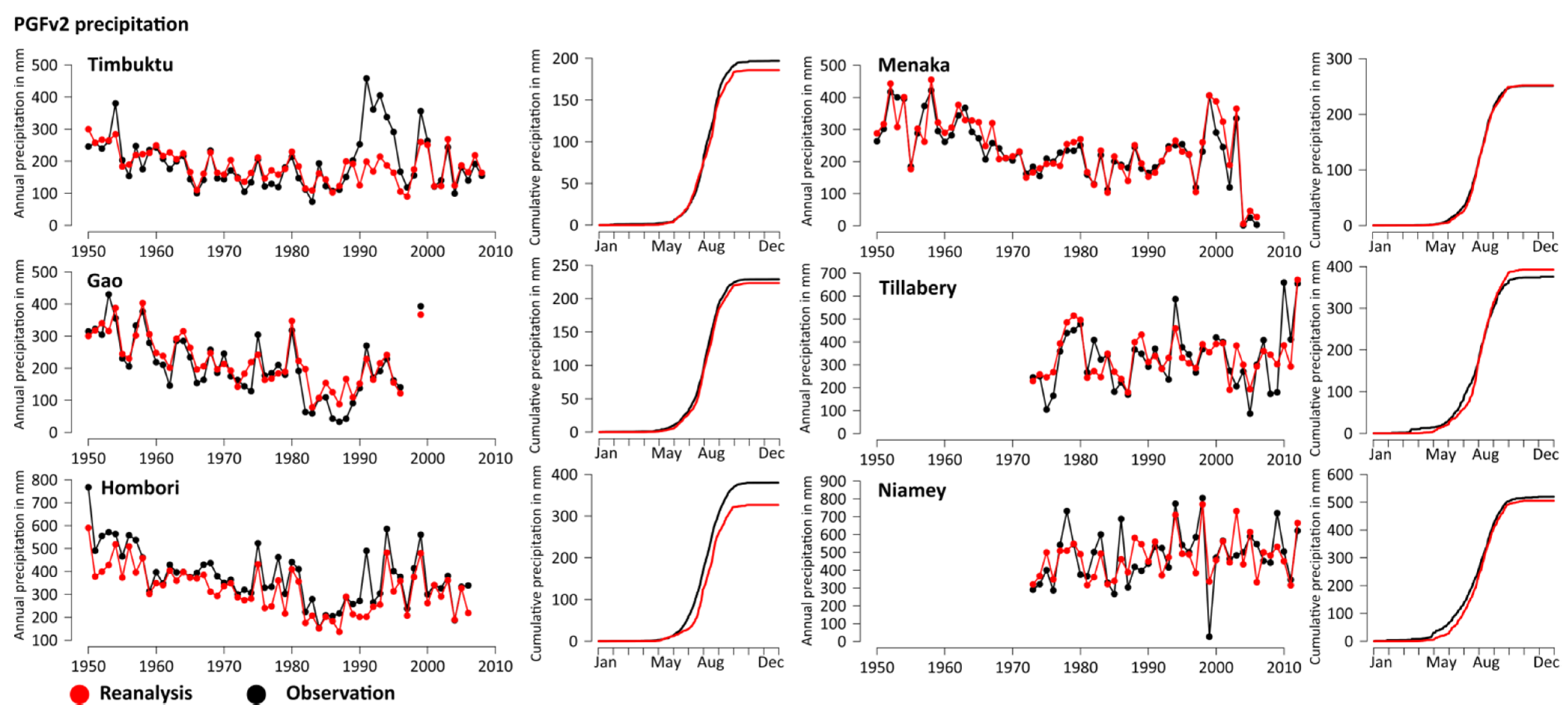
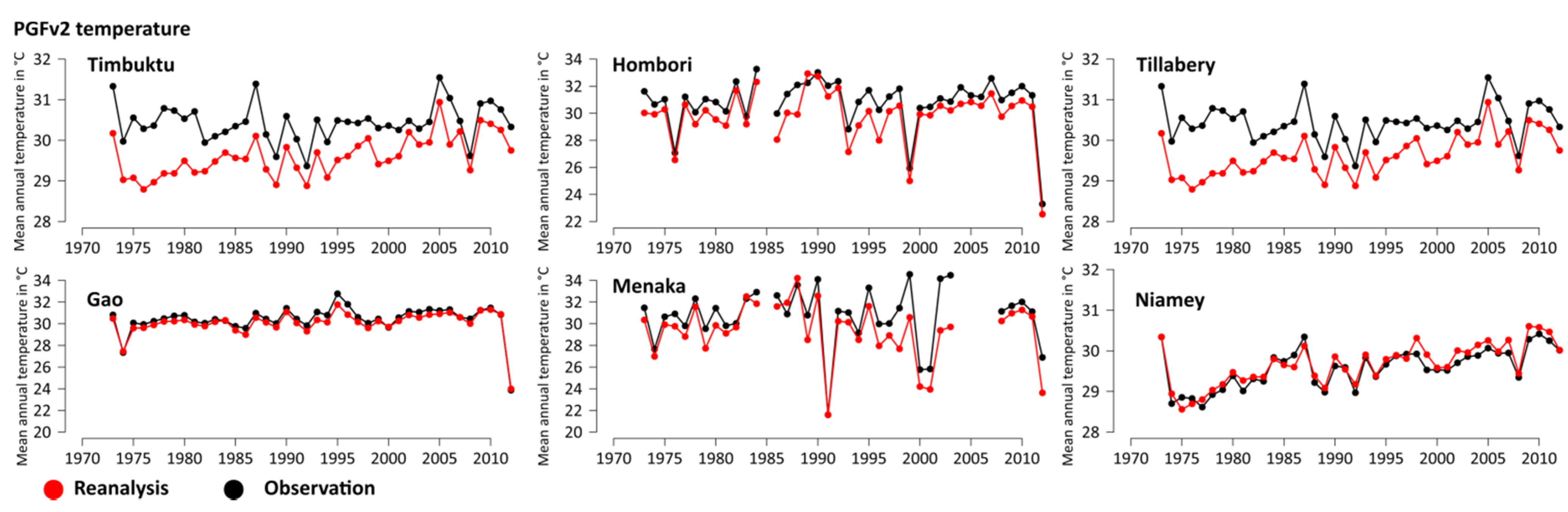
Figure 5) have been selected as potential model input. The visual comparison of temperature and precipitation shows that all of the data sets generally have good correspondence with the measured data, yet also all of them have some deficits (PGFv2:
Figure 4 and
Figure 5, WATCH:
Supplementary Material Figures S1 and S2, GSWP3:
Figures S3 and S4). Regarding precipitation, distinct deviations of single years or short periods do occur, as for example in all three data sets for the station Timbuktu during the early 1990s. However, the general trends in precipitation are represented in all three reanalysis products. Annual mean temperatures only rarely deviate more than 1 °C from the observed station data and reproduce the general trends also efficiently. Additional uncertainty derives from the limited evaluation. The comparison only takes six stations into account for the whole region. These points cannot represent the whole area. These uncertainties deriving from the climate data have to be taken into account when discussing the modeling results. The comparison implies that single years should not be compared between the modeling results and observations of discharge. However, since the major trends of the climate data are represented in the analysis, the climate data can be used for reproducing general trends with the model when results are carefully interpreted.
Figure 4.
Comparison of precipitation from interpolated PGFv2 reanalysis data (red) with observations from six weather stations (black) in the research area. For each station, the annual precipitation (left) and the cumulative sum of the precipitation of the whole period (right) is depicted.
Figure 4.
Comparison of precipitation from interpolated PGFv2 reanalysis data (red) with observations from six weather stations (black) in the research area. For each station, the annual precipitation (left) and the cumulative sum of the precipitation of the whole period (right) is depicted.
Since no systematic differences could be detected with regard to data quality, the PGFv2 data set was finally selected since it is the newest of the three data sets. It is a combination of a suite of global observation-based data sets with the National Centers for Environmental Prediction—National Center for Atmospheric Research reanalysis. The spatial resolution is at 0.5° × 0.5° and for the modeling the 3-hourly data has been aggregated to daily data.
For the precipitation analysis, annual rainfall data is aggregated for each subcatchment (Niger, Sirba, Goroul) by building the mean over all data points in the subcatchment region (
Figure 1). Since the Guinean Flood is completely generated in the Upper Niger basin, the related rainfall data was aggregated for this region outside the research area.
Figure 5.
Comparison of mean annual temperature of interpolated PGFv2 reanalysis data (red) with observations from six weather stations (black) in the research area.
Figure 5.
Comparison of mean annual temperature of interpolated PGFv2 reanalysis data (red) with observations from six weather stations (black) in the research area.
2.4.2. Discharge Data
Observed discharges from three monitoring stations (
Figure 1) were used to calibrate and validate the model and for the analysis of the AMAX. The observed discharge at the Diré station was used as input for the model (see
Section 2.2). The observations are part of the Niger-HYCOS monitoring network, managed by the Niger Basin Authority, which consists of daily water-level readings at more than 100 locations across the basin, as well as accompanying rating curves to compute discharge at these locations [
42].
The AMAX for the time series of Alcongui on the Goroul River and Garbe-Kourou on the Sirba River are created by selecting the highest daily discharge per year, with gaps for years where the peak cannot be identified due to missing values. The time series for Niamey has two peaks per year (see
Section 2.1). The second, the Guinean peak, occurs in most of the years after the 31st of December but is still assigned to the rainy season of the previous year. For the Red Flood, the procedure is not straightforward since the peak cannot be distinguished in dry years hidden from the Guinean Flood and thus it cannot be quantified for all years (see
Section 2.1). For the simulation, this problem was solved by simulating the discharge without the inflow of Diré, leading to a clear AMAX value of the Red Flood, generated in the Sahelian part of the Niger basin after Diré. For the observation, it is not possible to filter only the discharge which is generated in the basin downstream of Diré. Therefore, identification of the AMAX depends on a clearly distinguishable first peak of the hydrograph between July and October. For years when the flood peak cannot be detected since it is too low and hidden under the Guinean flood peak, the AMAX time series contains gaps, which affects the statistical analysis (see
Section 2.7).
2.4.3. Land Cover and Land Use Change Data
For the representation of the LULC in the model, maps of the land cover for different periods are needed. For this study, land use maps have been generated in five year steps from 1950 until 2005. There is no data available which provides this information to the degree of detail necessary for ecohydrological modeling at the meso-scale with regard to land classes. Therefore, the land cover maps have been derived using the information from two different data sets. In the first step, a base map was derived which has the necessary details concerning land cover at a fine spatial resolution. For the base map, land class information was derived from the GLC2000 data set [
43]. It differentiates between 27 land classes and has a spatial resolution of
, which corresponds to 1 km at the equator. It is based on remote sensing data and includes a detailed legend. The GLC2000 classes occurring in the research area have been transformed to the classes of the ecohydrological model (
Figure 1, see
Section 2.2).
However, this map only represents the one point in time at which the data was collected (year 2000). Therefore, an additional data set was used which gives information about the change in land cover with regard to crop, pasture, and urban land but for different times in history. The information on areal changes in crop and pasture was obtained from the Land-Use Harmonization project [
23]. The harmonized land use scenarios connect historical reconstructions with future scenarios and have been used as a basis for the Earth System Models of the fifth Assessment Report of the Intergovernmental Panel on Climate Change (IPCC). The historical data for the period 1500–2005 are based on the model HYDE [
44,
45], and contain information on changes to cropland, pasture and urban land at a 0.5° × 0.5° resolution on an annual basis. The reconstruction of the data set is based on satellite maps for the years they were available and for the more distant past by combining information on population density, soil suitability, distance to rivers or lakes, slopes, and specific biomes. Each grid point of the LULC data contained the percentage of crop, pasture and urban land (
Figure 2).
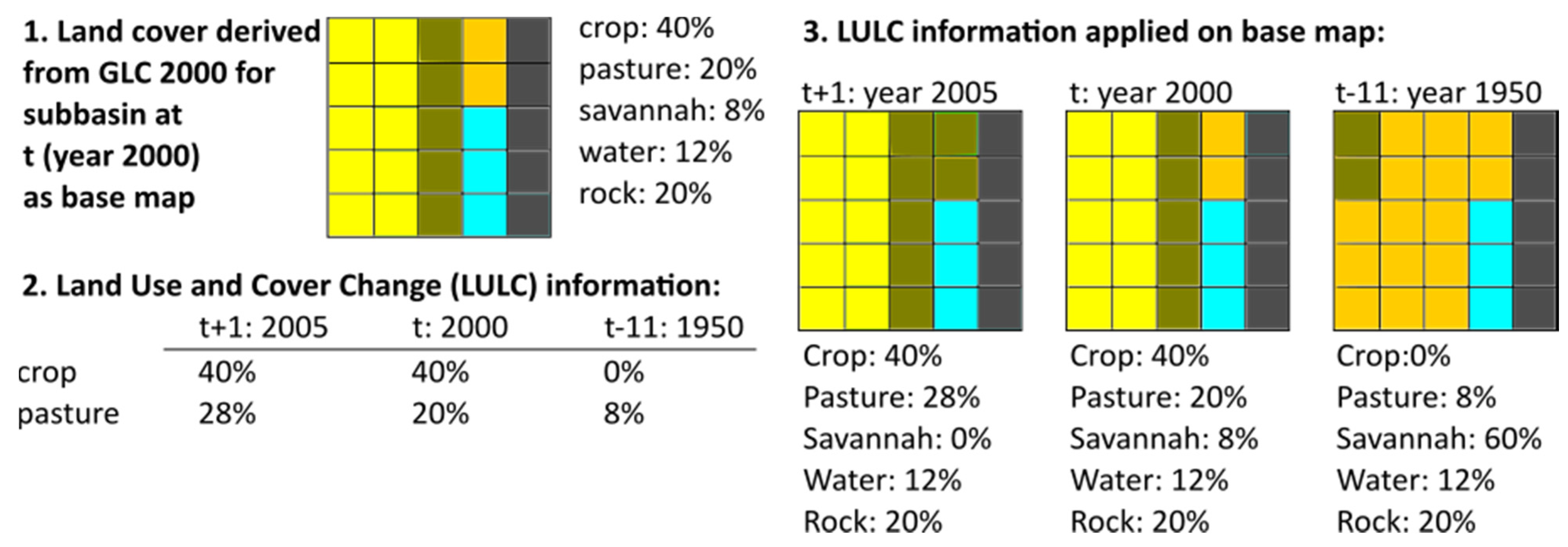
With this information on changes, the base map was altered for each of the 5-year time steps in order to have land use maps which represent the LULC, as shown simplified in
Figure 6. The LULC information was added to the base map on the subbasin level of the model, and existing land classes changed accordingly. The land classes of water, wetlands, sandy/stony desert and bare rock have been kept constant in the year 2000. When pasture, crop and/or urban land increase in a subbasin, other natural vegetation land classes like savannah or forest are proportionally reduced in the same subbasin. If crop, pasture and/or urban land decrease, the land classes of the natural vegetation increase proportionally.
Figure 6.
Exemplary process of how the information from the Land Use and Land Cover data of the Land-Use Harmonization project is used on the subbasin level to produce land cover maps for the different years which are then used by the land use change module. The whole square represents one exemplary subbasin, with small squares representing individual stable units (SU).
The emerging land class maps from 1950 until 2005 are used in the model as explained in
Section 2.4. In
Figure 3 the changes are quantified for the watershed of Niamey until Ansongo, corresponding to the area marked by climate grid points in
Figure 1. The related spatial distribution is shown in
Figure 2.
Crop types were derived from a data set for West African crops [
46]. The four main types in the region are millet, sorghum, cowpea and rice. For every subbasin, the same crop type has been used for the whole period, according to the dominant crop in the data.
2.4.4. Soil and Topographic Data
Information on the soils in the research area for the modeling was derived from the Digital Soil Map of the World [
47]. Relevant parameters for the model include depth, clay, silt and sand content, bulk density, porosity, available water capacity, field capacity, and saturated conductivity for each of the soil layers. For the delineation of the subbasins and necessary topographic information, a Digital Elevation Model derived from the Shuttle Radar Topography Missions at a 90 m resolution [
48] was used.
2.5. Calibration of the Model
An accurate representation of the main hydrological processes and characteristics of the research is a crucial precondition for a robust modeling attribution. Therefore, the model was calibrated with a standard procedure for SWIM and SWAT [
49] via an automatic calibration using the PEST software package [
50]. This is commonly applied, as for example done in the studies of Vetter
et al. [
38] on the rivers Rhine (Europe), Upper Niger (Africa), and Upper Yellow (Asia). The calibration was done individually for the Sirba (station Garbe-Kourou), the Goroul (station Alcongui) and the rest of the subcatchment between Diré and Niamey (station Niamey) to take into account the distinctly different geographic attributes. During the calibration, the LUCM was used in order to calibrate/validate the model with correct land use for the respective period and region. The calibrated parameters/factors are static and do not change within a subcatchment and over time. The focus of the calibration and model set-up for all subbasins was to achieve adequate efficiency for streamflow simulations on daily time steps, especially for high flows. Therefore, the main parameters/factors for the calibration were related to groundwater, river routing, saturated conductivity and potential evapotranspiration (
Table 1). For the Sirba and Goroul catchments, the parameters related to groundwater and the factors for potential evapotranspiration and saturated conductivity showed the highest sensitivity. Routing parameters were somewhat less sensitive. For the Niger basin between Diré and Niamey without the subcatchments of Goroul and Sirba, the sensitivity for the routing and the potential evapotranspiration was higher and the sensitivity of other parameters lower. This is likely due to the fact that the model is fed monitored data from the Diré gauging station (see
Section 2.2). Prior to the calibration, the available observed discharge data was checked visually and calibration periods were selected where distinct high and distinct low annual peaks are represented in order to cover a broad range of rainfall-runoff conditions. The period was finally selected when a period of eight years with a low amount of missing data was available (Goroul (Alcongui): 1963–1970, Sirba (Garbe-Kourou): 1986–1994, Niger (Niamey): 1988–1995). The validation periods are before or after the calibration period, depending on the availability of observations (Goroul (Alcongui): 1971–1978, Sirba (Garbe-Kourou): 1978–1985, Niger (Niamey): 1996–2003). Since there are not enough climatic observations available, reanalysis data is used to drive the model, also during the calibration. The results of the calibration are shown in
Table 2.
Table 1.
Calibrated parameters of the ecohydrological model SWIM (Soil and Water Integrated Model) with a short description.
Table 1.
Calibrated parameters of the ecohydrological model SWIM (Soil and Water Integrated Model) with a short description.
| Calibrated Parameter/Factors | Short Description |
|---|
| Groundwater related parameters | Groundwater recession | Rate at which groundwater flow is returned to the stream. |
| Groundwater delay | The time it takes for water to leave the bottom of the root zone until it reaches the shallow aquifer where it can become groundwater flow (in days). |
| Baseflow factor | The baseflow factor is used to calculate the return flow travel time. The return flow travel time is then used to calculate percolation in the soil from layer to layer. |
| Correction factor for saturated conductivity | The factor is applied for all soils |
| Correction factor for potential evapotranspiration | The factor is applied for all subbasins in the respective subbasin. |
| Routing coefficient | Routing coefficient to calculate the storage time constant of the flow from the initial estimation which is based on channel length and celerity. |
Table 2.
Calibration and validation results of the eco-hydrological model SWIM in Nash-Sutcliff efficiency (NSE) and percent bias (PBIAS) for three stations.
Table 2.
Calibration and validation results of the eco-hydrological model SWIM in Nash-Sutcliff efficiency (NSE) and percent bias (PBIAS) for three stations.
| Gauging Stations | Calibration | Validation |
|---|
| NSE | PBIAS | NSE | PBIAS |
|---|
| Alcongui (Goroul) | 0.58 | −0.4 | 0.55 | −16.9 |
| Garbe-Kourou (Sirba) | 0.66 | 22.1 | 0.49 | 34.5 |
| Niamey (Niger) | 0.86 | 12.2 | 0.87 | 6.9 |
2.6. Sensitivity Analysis of the Effects of LULC on the Hydrological Regime
The representation of the LULC and their effect on the hydrological processes are important for an understanding of the discharge changes. In
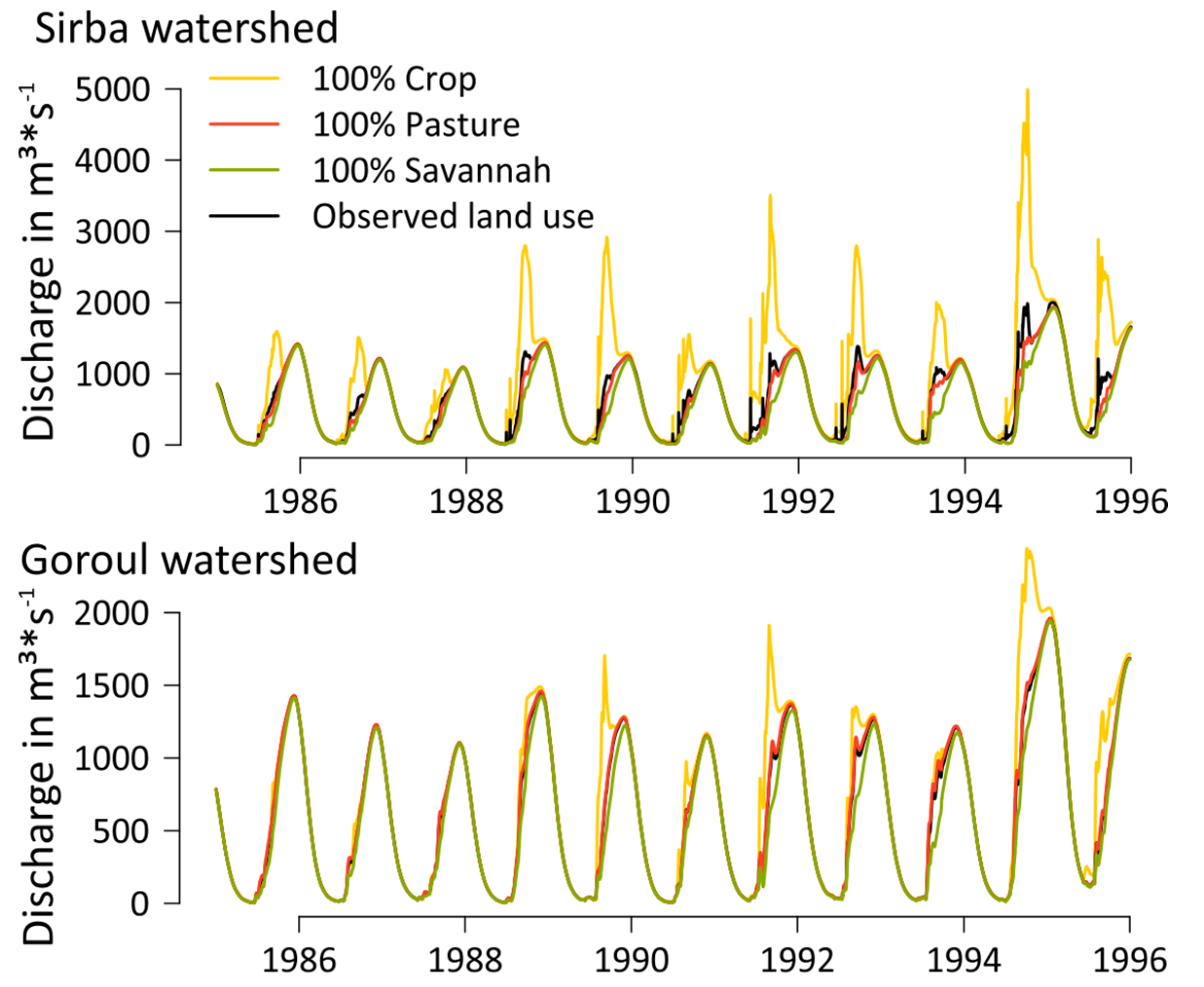
Figure 7, the effects of different land cover on the modelled hydrological regime are shown for the Sirba and Goroul watersheds. The watersheds have been modelled with three set-ups, with either crop, pasture or savannah vegetation covering the entire subcatchments. The model is run for a period of 10 years (1985–1995). Regarding precipitation, the 10-year period was selected with a rather dry beginning and above-average wet conditions at the end in order to allow for different rainfall-runoff conditions.
The subcatchments covered solely with crops show a strong increase in peak discharges. In the wetter Goroul catchment, this holds true even for the dry years at the beginning of the 10-year period. The results for crop cover correspond to the changes as described in detail in Amogu
et al. (2010) [
22], Descroix
et al. 2012 [
3] and Descroix
et al. 2013 [
4] for the research area. The LULC processes lead to a decrease in infiltrability and more direct runoff and regeneration of groundwater. They attribute the regeneration of the groundwater to the fast infiltration in the rivers, which carry more water due to the increase in runoff. This effects lead to a higher frequency of flow changes and flashiness. For pasture, this process seems to be much weaker in the modeling results.
These results reflect the sensitivity analysis of different studies of LULC in Africa, using the same land class parameters of the SWAT model. Awotowi
et al. (2014) [
33] show for West Africa that land use classes of SWAT are generally suitable for West African conditions. They found similar effects of LULC on the hydrology for the Volta basin, where cropland replaced savannah and grassland. Other studies undertaken with SWAT in East Africa studying the effects of LULC focus more on the transformation of forest to cropland [
34,
35,
51]. Concerning the effect of the transformation from savannah into pasture as taken place mainly in the Goroul catchment, it was not possible to test whether the parameterization of the model reflects the hydrological processes. There is no quantitative data or literature available to the authors which could be used to verify the modelled effects. The potential misparametrization of pasture is discussed in more detail in
Section 3.2 and
Section 3.3.
Figure 7.
Comparison of discharges with four different land use coverages (100% crop, 100% pasture, 100% Savanna and land use as observed) for the Sirba and Goroul watersheds.
Figure 7.
Comparison of discharges with four different land use coverages (100% crop, 100% pasture, 100% Savanna and land use as observed) for the Sirba and Goroul watersheds.
2.7. Statistical Methods
In order to make general trends of the time series more clearly visible, the local regression fitting technique LOESS was used [
52]. This is a nonparametric regression method that combines multiple regression models in a k-nearest-neighbor-based meta-model [
53]. When plotted, it generates a smooth curve through a set of data points. It is used to depict nonlinear trends in time series.
Since the absolute values of discharge differ distinctively between the different parts of the catchment, AMAX anomalies are used in order to make the results more easily comparable. The time series of AMAX anomalies is given by the time series of AMAX of the individual years divided by the mean AMAX of the entire AMAX time series of 1950–2009, given as a percentage. The annual rainfall time series are transformed to anomalies accordingly.
Linear trends in the observed and simulated AMAX time series are estimated using the Theil-Sen estimator [
54,
55]. It estimates the slope of a trend and is widely used, since it is insensitive to outliers. Since serial independence is a requirement of the test, the data was checked for autocorrelations using the Durbin-Watson statistic test [
56,
57]. It tests the null hypothesis that the residuals from an ordinary least-squares regression are not autocorrelated against the alternative that the residuals are autocorrelated. If an autocorrelation of the first order was found, trend-free pre-whitening was applied according to the method proposed by Yue
et al. (2002) [
58]. It is a procedure to remove serial correlation from time series, and hence to eliminate the effect of serial correlation on the Theil-Sen estimator.
As a result of the gaps in the time series for the Red Flood (see
Section 2.4.2), it is not possible to generate a local regression curve and to identify the minimum of the AMAX time series. The linear trends are therefore only calculated from 1984 to 2009 with five missing years (1986, 1987, 1993, 1995, 1996). This means that the AMAX trends are calculated consistently for the simulations even with these gaps and can therefore be included in the interpretation.
For the calibration and validation, the methods of Nash and Sutcliff (1970) (NSE) [
59], and percent bias (PBIAS) have been used. The NSE is calculated using the formula.
Values for the NSE range from 1 to negative ∞ values. An NSE of 0 means that the model is no better than using average annual discharge as a predictor. If NSE = 1, it means that the model is perfectly aligned with the observations. The PBIAS indicates the over- or underestimation of discharge during the calibration or validation period as a percentage. For the evaluation of the NSE and PBIAS the terminology of Moriasi
et al. [
60] is used (for NSE: very good: 0.75–1.0, good: 0.65–0.75, satisfactory: 0.5–0.65, unsatisfactory: <0.5; for PBIAS: very good: <|10|, good: |10|–|15|, satisfactory: |15|–|25|, unsatisfactory: ≥|25|).
2.8. Hypothesis Testing Framework
In order to attribute the increase of discharge observed in the research area to LULC and/or climatic changes, a simulation-based approach within a hypothesis testing framework as proposed by Merz
et al. [
5] is applied. The framework consists of the evidence of consistency, the evidence of inconsistency, and the provision of confidence level. In order to show the consistency or inconsistency, the observed trend is compared to the change simulated by the hydrological model, either with or without considering the potential driver LULC. The model which includes all postulated drivers, as in our case both changes in LULC and climatic regime, should be able to reproduce the observed trends and are therefore control runs. The simulations without one of the postulated drivers, might result in no trends or differing trends. This difference can then be used for the quantification of the influence. In other words, if the model is capable of simulating the observed trend without LULC, it would mean that LULC has no or little influence on the discharge trend and vice versa (within the uncertainty limits of model runs).
In this study, the observed trend is an increase of flood peak magnitude since the 1970s/1980s. Therefore, the AMAX is derived from the observed and simulated daily time series of discharge. The AMAX time series have been transformed from absolute values to anomalies (see
Section 2.7) in order to be able to compare the gradients amongst the subcatchments. The gradients of the trends are used as measure for the comparison. Ideally, the second/control run including LULC shows a similar gradient like the observed trend. The difference between the gradients of the run without LULC and the observed then consequently indicates the share of the climatic variability.
Annual rainfall is used as general indicator of the wetness trend in the respective watershed. The rainfall trend mainly helps to illustrate the SP (see
Section 2.1.), and whether the simulations are able to reproduce the phenomenon when including LULC.
3. Results and Discussion
3.1. Validation of the Model
To quantify the efficiency of the model, the NSE and PBIAS were used (see
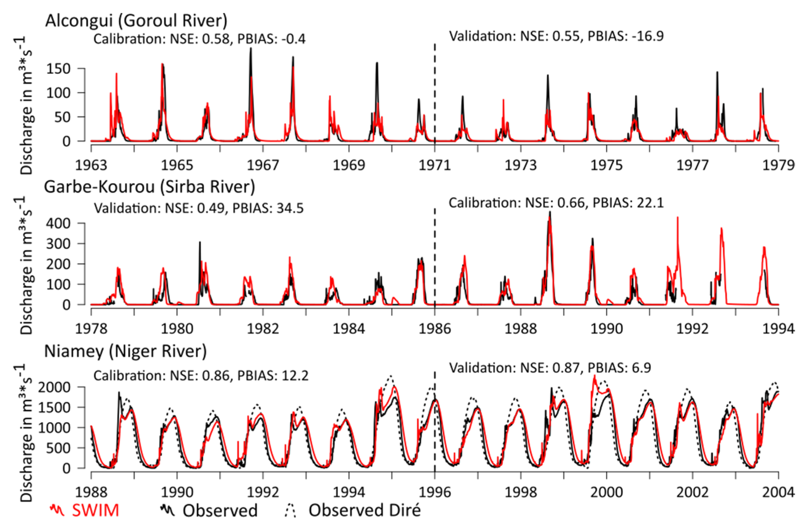
Section 2.7). The model showed very high efficiency at the gauging station Niamey for the validation period (NSE: 0.87/PBIAS: 6.9) (
Figure 8). For the Goroul basin, the results are satisfactory for the NSE (0.55) and slightly unsatisfactory for the Sirba basin (0.49). For the PBIAS, only the validation of the station Alcongui shows satisfactory efficiency (−16.9). At the station Garbe-Kourou, the PBIAS is over 25 and therefore unsatisfactory. The very good performance of the model for the station Niger can be explained by the fact that monitored data was fed into the model at the station Diré, while the reason for the weaker performance of the model in the watersheds of the Goroul and Sirba Rivers after the intensive calibration efforts is unclear. We assume that the climatic reanalysis data for these subcatchments are at above-average deficiency and/or that the land use data for these regions are not accurate. In fact, some years with similar observed hydrographs, like 1974 and 1975 at the Goroul river, for example, are simulated once very accurately and yet in the other year are deficient. An additional reason for the difficulties could be that the discharge of rivers in dry environments is generally more sensitive to climate input due to the low runoff-coefficients [
37], which is especially the case for the intermittent rivers Goroul and Sirba. Inaccurate climate forcing is therefore more likely to affect the model performance in drier regions. The reasons, therefore, are the proportionally higher losses in smaller streams through evapotranspiration, transmission losses,
etc. compared to large rivers. A certain decrease in rainfall thus leads to a proportionally larger decrease in discharge in dry areas compared to wetter areas [
37]. Other explanations for the lower performance might be data quality of the streamflow, the parametrization of the land use or other deficits in the model structure, e.g., for the representation of the groundwater. These input data related problems are taken into account in the discussion (see
Section 3.2 and
Section 3.3).
Figure 8.
Validation and calibration of the SWIM model for the watersheds of Alcongui, Garbe-Kourou and Niamey for eight-year periods using PGFv2 reanalysis climate forcing. For Niamey, the measured discharge at the Diré gauge is additionally plotted, which is fed into the model.
Figure 8.
Validation and calibration of the SWIM model for the watersheds of Alcongui, Garbe-Kourou and Niamey for eight-year periods using PGFv2 reanalysis climate forcing. For Niamey, the measured discharge at the Diré gauge is additionally plotted, which is fed into the model.
Since in this study absolute numbers of discharge are not analyzed but only anomalies, the NSE is more meaningful than the PBIAS. Therefore, the output of the model is used in the study for the Niamey gauge but also for the smaller subcatchments, with lower but still satisfying model efficiency, when looking at the calibration and validation phases.
3.2. Attribution of Trends in Annual Maximum Discharges
3.2.1. Simulation Results
The gradients of the trend lines for all AMAX anomaly time series are used as a quantitative attribution measure as specified in
Section 2.8. (see trend lines in the lower part of
Figure 9 and gradients in
Table 3) All estimated observed and simulated trends are positive and statistically significant (α = 0.05).
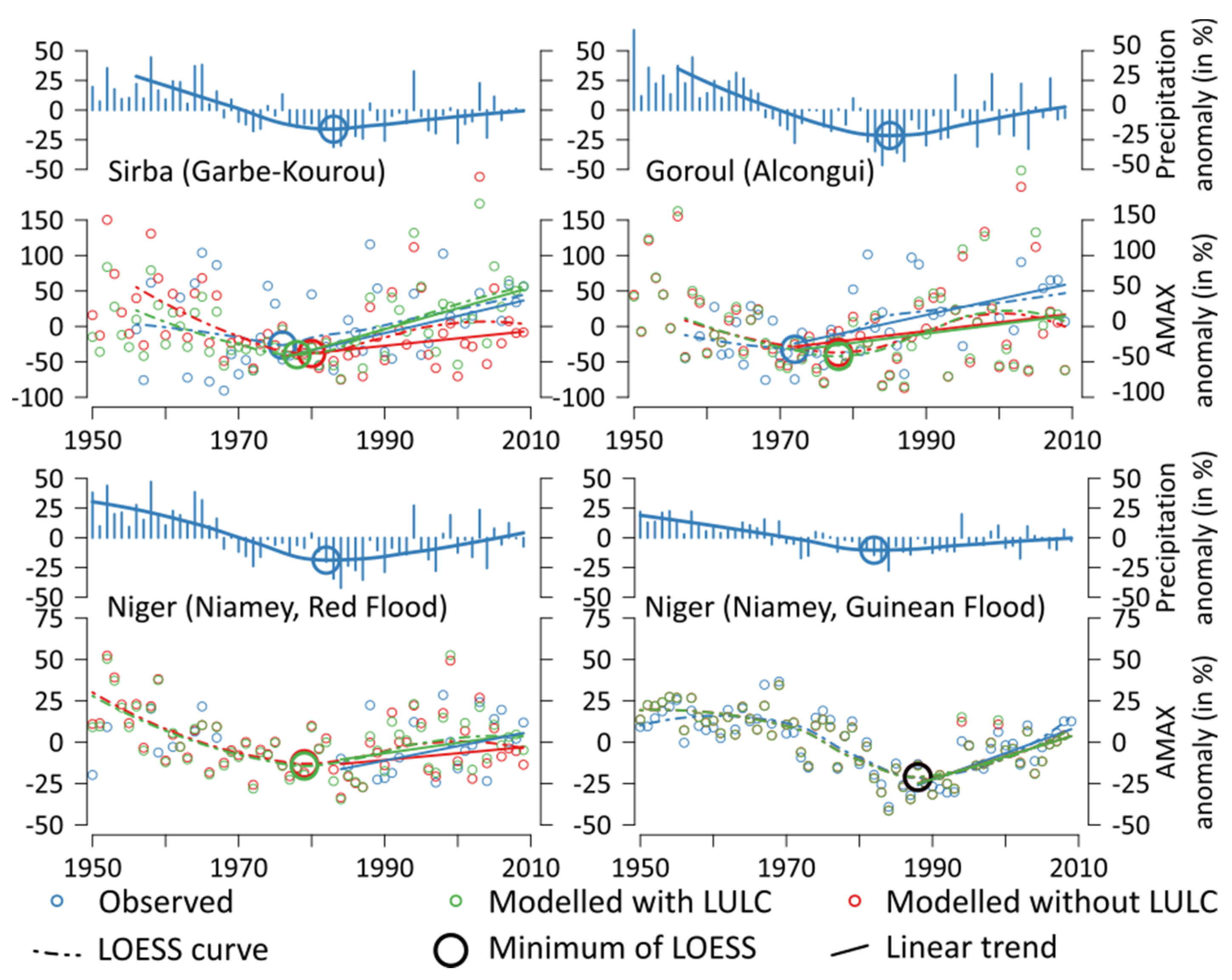
Figure 9.
Anomalies of annual maximum discharges for the gauging stations Alcongui (Goroul River), Garbe-Kourou (Sirba River) and differentiated between the Red and the Guinean Flood for Niamey (Niger River). On the top of each region, rainfall anomalies over the respective catchment are plotted. A LOESS curve with a minimum point is added as a dashed line and the Theil-Sen estimators for the discharge trends are plotted as bold lines, beginning at the minimum of the observed discharge points. Please note that, for the observed values of the Red Flood at Niamey, the time series is incomplete (see
Section 2.4.2). Therefore, the LOESS curve is not plotted and the trends start at 1984 (see
Section 2.6). For the Guinean Flood at Niamey, all minima are on the same point and the circle is plotted in black.
In the Sirba catchment, the simulation run including LULC reproduces the trend of AMAX anomaly adequately (sim
with LULC: 2.94, obs.: 2.42,
Table 3), whereas the simulation run that assumed no LULC since 1950s does not reproduce the observed trend of AMAX anomaly adequately (sim
without LULC: 1.05).
Table 3.
Gradient of the trends of AMAX anomalies (see
Figure 4) as estimated with the Theil-Sen approach.
Table 3.
Gradient of the trends of AMAX anomalies (see Figure 4) as estimated with the Theil-Sen approach.
| Gauging Stations | Observed | Simulation w. LULC | Simulation w/o LULC |
|---|
| Gradient | % of Observed Gradient | Gradient | % of Observed Gradient |
|---|
| Sirba River (Garbe-Kourou) | 2.42 | 2.94 | 121% | 1.05 | 43% |
| Goroul River (Alcongui) | 2.37 | 1.38 | 58% | 1.29 | 54% |
| Niger River (Niamey, Red Flood) | 0.87 | 0.63 | 72% | 0.56 | 64% |
| Niger River (Niamey, Guinean Flood) | 1.61 | 1.37 | 85% | 1.36 | 84% |
In contrast, for the Guinean flood of the Niger River at Niamey, the AMAX anomaly gradients of both simulations are similar to the observed trends of the AMAX anomaly (simwith LULC: 1.37, simwithout LULC: 1.36, obs: 1.61). For the so-called Red Flood of the Niger River at Niamey, the simulation with LULC is closer to the observed AMAX trend than the run without considering LULC (simwith LULC: 0.63, simwithout LULC: 0.56, obs.: 0.87), but both are not able to reproduce the trend adequately.
In the Goroul catchment, the gradients of both simulation runs (simwith LULC: 1.38, simwithout LULC: 1.29, obs.: 2.37) significantly underestimate the observed gradient of AMAX anomalies.
The Sahel Paradox (SP) of the Sirba catchment is distinct with an offset between the minima of AMAX and annual rainfall of approximately 10 years. Both simulations show this effect while the SP of the control run is more distinct, with an AMAX minimum close to the observed AMAX minimum.
In the Goroul catchment the SP is very pronounced, too, with an offset of approximately 14 years. Both simulations show the effect while they underestimate the offset by approximately seven years. For the Red Flood at Niamey, it is not possible to detect the magnitude of the SP shift of the observed AMAX due to the missing LOESS curve and minimum (see
Section 2.7). However, both simulations show an offset of around five years, which is in accordance with the findings from the Sirba River. For the Guinean Flood the effect of the SP does not occur and rainfall and AMAX minima do not show the paradoxical offset.
3.2.2. Discussion of Simulation Results
The effects of LULC are most pronounced in the model runs for the Sirba subcatchment. The main LULC in this watershed is a distinct increase in cropland and a reduction of natural savannah (
Figure 3). This leads to an increase of surface flow and less evapotranspiration, both represented in the model parametrization. Because the run without LULC generates a trend gradient of 43% of the gradient of the observed trend, this share can be attributed to the climatic changes and, consequently, the other half to the LULC.
The Guinean Flood is almost exclusively controlled by the hydrological setting upstream of the Sahelian Niger. Since this study only simulates the basin downstream of Diré, the LULC effects upstream are not simulated. If there were effects, they are inherent in the observed discharge which was fed into the model at Diré. Still, the absence of any LULC effect when flowing through the Sahelian part, as well as the correlation between the rainfall and the AMAX trends, supports the finding of Aich
et al. [
1]. They identified the climate as the main driver of the Guinean Flood. The differences between the trend magnitudes of rain and AMAX can be explained by the sensitivity of the Niger basin, which causes a higher increase in discharge compared to the magnitude of rainfall [
37].
For the Red Flood of the Niger River at Niamey, there is almost no difference in the gradients of the simulations with and without LULC. The runs without LULC and hence with only the climatic forcing causing the trend can explain 64% of the observed AMAX anomaly trend. The modelled effect of LULC is small and reproduces 72% of the observed trend. These results of the Red Flood correspond to the results of the Goroul catchment, which is the beside the Sirba catchment the second major tributary catchment generating the Red Flood (see
Section 2.1). Therefore they are discussed together.
In the Goroul catchment, the poor performance of the model runs with and without LULC only allows a partial quantification of the relative effect of the drivers. Following the simulation results without LULC, the climatic part of the simulations explains 54% of the observed trend gradient. The cause for the remaining 46% is unclear, since the runs with LULC do not reproduce the trend significantly better. Therefore, it is not possible to give robust statements for the Goroul catchment and for the Red Flood as to the influence of the assumed drivers and quantification is a fortiori uncertain. The results might even indicate that there is an additional driver forcing the AMAX trends besides climatic changes and LULC, which is not represented in the model and has not been postulated. Another general point is the quality of the observed discharge data and the reanalyzed climate data. Especially in the Goroul catchment, the validation shows that some peaks are missed completely by the model (e.g., Alcongui 1977), or that peaks which are modelled do not occur at all in the discharge data (e.g., Alcongui 1963). This indicates the general deficit of the employed observed reanalyzed data and needs to be taken into account for the interpretation as well. However, a more probable explanation is the combination of inadequate information on LULC and/or a deficient representation of LULC in the model. The dominant change in the reanalysis data set of LULC in the watershed is a transformation of savannah to pasture (
Figure 2). These two land cover types do not differ substantially in their modelled effects on the hydrological regime (see
Section 2.6,
Figure 7). Therefore, the similar and poor results for the runs with and without the LUCM are a logical consequence. The parameters for pasture of the SWAT land class parameters are most likely optimized for pastures in the temperate zone. The hydrological effects of pasture in the Sahel differ probably from these temperate pastures. However, since no other data was available to the authors in order to check or even change the effects and the related parameters of pasture in the Sahel, this deficit could neither be verified nor corrected. We assume that especially the infiltration capacities of Sahelian pastures are lower than of pastures in the temperate zones, e.g., due to soil-crusting effects and less dense vegetation. An additional source of uncertainty is the undifferentiated information on LULC with regard to savannah. Descroix
et al. (2012) [
3] describe the LULC of this region with a change from the original bushy and woody savannah to a degraded savannah (Tiger Bush, see
Section 2.1) and sandy slopes due to land clearing. These changes are not represented in the LULC data (see
Section 2.4.3).
The SP is a special aspect of the increase of flood magnitudes. Following our results, the same statements and explanations, which can explain the increase in flood magnitude, hold also for the SP. For all time series (except the ones from the Guinean Flood of the Niger River at Niamey, where the SP did not occur), the SP phenomenon could be reproduced without LULC, but to a lower degree than when accounting for LULC. We assume that this effect is based on changes in the frequency of precipitation in the climatic forcing. The findings of Panthou
et al. [
61,
62] of increasing convective precipitation supports this theory that heavy precipitation leads to an increase of the run-off coefficient, and finally to an increase in discharge. This effect is also shown by means of measurements in Amogu
et al. [
22]. Eventually, the combined actions of LULC and changes in precipitation patterns seem responsible for the observed SP in the 1970s/1980s.
Another finding is the non-stationary influence of climate. The model runs without LULC, and hence with only climate as the driver show upward trends in AMAX for both tributaries and the Red Flood of the Niger River at Niamey. These increases are, however, stronger than the respective annual rainfall anomalies would suggest. Therefore, we assume that changes in the rainfall patterns, most likely an increase in the frequency of heavy precipitation, contribute to the trend. This is supported by state-of-the-art analysis of climatic changes in the Sahel, for example by Panthou
et al. [
61,
62].
3.3. Discussion of the Methodological Framework Employed and Related Uncertainties
We acknowledge that simulation runs and the calibration procedure are affected by a wide range of uncertainties regarding the processes in the model, their parametrization and the driver data. Relevant processes like evapotranspiration and surface runoff are not entirely physically based in the model but simplified and calibrated with a factor or empirical (e.g., the factor for potential evapotranspiration and the curve number approach). Therefore, the effects of LULC on these processes could be represented inadequately. However, the SWIM model showed in this study, like SWAT model in other LULC studies in the region [
33], that the process-based models are generally able to reproduce the effects of LULC.
The data on LULC as the key driver of the attribution study cannot be easily improved regarding temporal and spatial resolution since no other data products or observation on LULC are available for the region. There is only a qualitative confirmation of the used LULC data by studies which are based on observations [
3,
22]. The global LULC data set seemed therefore partly reliable, but, for example degradation of savannah (Tiger Bush, see
Section 2.1), as reported in the studies are not represented in such a detail. We therefore recommended for similar studies the use of regional and more detailed data sets, if available.
Regarding the uncertainty coming from the parametrization, especially the representation of land cover types in the model has to be adequately included in terms of their hydrological attributes. The robustness of a simulation-based attribution study is therefore not only dependent on the general validation results of the model, but rather on the ability of the model to reflect well-known changes of the postulated driver(s) adequately. Especially the parametrization of pasture in the model is questionable, but could, due to the lack of related field data, not be improved. A way to avoid this uncertainty might be the calibration of each of the main changing land cover types separately by looking at small catchments which are dominated by one of these land uses [
63]. In doing so, the sensitivity of the model against the impact of each change can be verified and tested whether the representation is adequate or not. Unfortunately, discharge data for the validation of the model performance on such homogeneous areas were not available for the research area of this study.
Additional uncertainty is related to the general methodological framework. A modeling attribution study only can provide robust results, if all potential drivers of the observed change were adequately represented in the model. Two drivers, LULC and climatic changes, which are mentioned by qualitative studies as potential sources for the increasing flood trend [
3,
22] are tested in this study. However, we cannot exclude the influence of a third or more drivers for the observed changes. For example the effects of the extreme population growth in the region, might influence the hydrological regime, possibly via sealing of soils near settlements. Still, the two considered drivers LULC and climate are the only potential drivers in the current literature of the Niger, which makes the assumption more reliable.
Also the assumption of linear trends in the AMAX anomaly time series and accordingly in the LULC and climatic changes is probably not realistic. However, comparing non-linear trends would request an even higher level of data quality/density, which is not available in the research area.
Another critical issue is model performance with respect to other important state variables of the model like groundwater flows and evapotranspiration. In this study, the performance of the model was only tested with regard to discharge, since no quantitative data was available on groundwater dynamics. However, in the Sahelian part of the Niger, groundwater is known to play a crucial role [
64] and it cannot be excluded that the model underestimates the effects of a potential relevant process related to LULC.
However, keeping model uncertainty in mind—Even under conditions of comparatively poor data quality and availability, the simulation-based approach using a process-based based model, shed new light on attribution of increasing floods in the Sahelian part of the Niger by developing some first quantitative measure of comparing the linear trend estimates of AMAX anomalies. In addition, even without adequately representing the LULC in the Goroul catchment and for the Red Flood at the station Niamey, the method could show that at least climatic changes contribute substantially to the flood increase in the region.
4. Conclusions
The research question, to which share LULC and/or climatic changes cause the increase of flooding in the Sahelian part of the Niger basin, can only be answered partly by this study. The most reliable conclusions can be drawn from the results of the Sirba catchment, since the simulation including LULC is able to reproduce the observed trend adequately. The influences of both drivers on the observed trend of AMAX seem to be roughly equal with a share of 43% which can be—within the known limitations—attributed to the climatic changes.
For the Goroul subcatchment and the Red Flood of the Niger River, the results are in the same order of magnitude with shares of the climatic forcing of 54% (Goroul) and 64% (Niamey Red Flood). Since the model was not able to reproduce the influence of LULC adequately, the results for these two stations are uncertain and only partly reliable. For Goroul and the Red Flood, we conclude that climatic changes have A major influence on the observed trend of AMAX and LULC also contributes, but to an unknown amount.
Using a process-based eco-hydrological model seems to be a valid method for attributing an increase of flooding. Even though main processes related to LULC, like e.g., evapotranspiration, are simplified and calibrated in the model or empirical like the curve number approach for surface runoff, the effects of LULC on the hydrology are assumed to be generally well represented since the modelled effects reflect observed effects and other studies could show a general suitability of process-based models for LULC studies. Still we see a general need for hydrological science to overcome the calibration of land use sensitive parameters in favor of more physically-based models, especially for LULC studies. These efforts are, however, still limited by data availability, computing power and partly also detailed process understanding.
In regard of the specific methodology applied in this study, the gradient prooved to be an uncomplicated and intuitive measure for comparing simulated and observed trends and estimating the influence of different drivers. However, the demands for a robust attribution on the model and data quality/density are high. Testing the method in a data-richer environment, where especially more information on LULC are available, would help to get a better understanding of its robustness and reliability.
Regarding flood mitigation and adaptation strategies, the modeling framework could be employed to assess different land management options. If the flood risk is to a significant extent due to LULC (rather than due to a climatic change), it means that it can also be counteracted. State-of-the-art options implemented locally can reduce surface runoff, for example, by reforestation, smart planting techniques which also reduce erosion, shifting cultivation
etc., such as those published in the World Overview of Conservation Approaches and Technologies (WOCAT) [
65] or weADAPT [
66]. However, in the face of the existing flood risk in the region and the return to wet conditions, mitigation is not enough. There is a strong need for immediate adaptation measures and we argue for early-warning systems, investments in flood protection infrastructure and flood-smart settlement policies in the riverine nations. To ensure cost-efficient implementation, a simulation-based approach can be further used to assess the relative merits of both mitigation and adaptation measures [
67].


 ,
, 


