Article

Exploring the Modifiable Areal Unit Problem in Spatial Water Assessments: A Case of Water Shortage in Monsoon Asia

Water & Development Research Group, Aalto University, Tietotie 1E, Espoo 02150, Finland
*
Author to whom correspondence should be addressed.
Water 2015, 7(3), 898-917; https://doi.org/10.3390/w7030898
Submission received: 4 November 2014 / Revised: 13 January 2015 / Accepted: 27 February 2015 / Published: 3 March 2015

Abstract

:
Water shortage (availability per capita) is a key indicator of vulnerability to water scarcity. Spatial datasets enable the assessment of water shortage on multiple scales. The use of river basins and subbasins as analysis and management units is currently commonplace. An important but less acknowledged fact is that spatial assessments are strongly influenced by the choice of the unit of analysis due to the Modifiable Areal Unit Problem (MAUP). Climate conditions, agricultural activities, and access to groundwater also influence water availability and demand. In this study, a total of 21 different criteria were used to define areal units of analysis, i.e., zonings, for which water shortage was calculated. Focusing on Monsoon Asia, where water scarcity is a pressing problem, we found that zoning had a considerable impact, resulting in up to three-fold differences in the population under high water shortage (<1000 m3/cap/year), ranging from 782 million to 2.11 billion. In most zonings, however, the Indus and Yellow River Basins and northwest parts of India and China are under high water shortage. The study indicates that a multizonal and multiscale analysis is needed to minimize skewed or even misleading information that might be produced when using only one zoning.

1. Introduction

Spatial assessments are used to support the management of water resources and the environment [1,2,3,4,5,6,7,8]. Spatially varying distribution of population growth, changing water consumption, and changing climate have made water scarcity one of the key concerns in the world [4,9]. Globally, almost half of the population is living under some sort of water scarcity [10] and this proportion is predicted to grow in future [11]. Water scarcity is particularly pressing in South Asia as well as in East and Southeast Asia (referred to in this study as Monsoon Asia), where over half of mankind lives, and where a large portion of food production is affected by a highly variable climate [12,13].
Water scarcity, in terms of blue water, can be divided into physical and social scarcity [14]. Physical scarcity can further be divided into water shortage (water availability per capita) and water stress (water use relative to availability) [14]. The water shortage indicator—for which results are shown in this article—is the most widely used indicator of water scarcity in spatial vulnerability studies, thanks to its simplicity [14,15,16,17,18,19]. It provides important information on the ability to physically provide for major water requirements of households, the agriculture, industrial, and energy sectors, as well as the environment [14,20]. At the same time, we acknowledge the limitations of the indicator. In particular, examining the annual average runoff overlooks scarcity at shorter periods within the year, and excluding the influence of infrastructure and variations in demands causes inaccuracies e.g., [19].
Global models provide gridded spatial datasets e.g., [21,22,23,24] of available water resources and population, which enable water shortage calculations for various spatial levels with numerous areal units of analysis. The most popular of these levels and units of analysis include administrative units e.g., [20,25,26] and hydrological basins e.g., [9,26], or a combination of these e.g., [27,28]. In addition, assessments have been conducted at the level of grid cells e.g., [29,30]. However, other possibilities exist. For example, water shortage could be examined according to different agro-ecological zones, groundwater basins, or accounting for differences in climate [28,31].
The criteria used to define the areal unit of analysis influences the results of spatial assessments e.g., [11,19] due to the Modifiable Areal Unit Problem (MAUP) phenomenon [32,33,34]. The MAUP can be observed through two effects, one caused by scaling and the other by zoning (see Section 2 for more details). The MAUP was discovered in the 1930s [35], and many studies have handled the issue since then [33,34,36,37,38,39,40,41,42,43,44]. Though this phenomenon concerns practically any research using geographic or spatially-referenced data, it has been relatively little discussed [32,34], particularly in water resources management [15,16,17]. As the MAUP can result in substantial differences in conclusions and recommendations for action, it is a major concern for policy making and planning. Perveen and James studied the scaling effect with water shortage and stress indicators [15,16,17], but to our knowledge the zoning effect for spatial water-related assessment results has not yet been systematically explored.
This study aims to address this research gap by examining the zoning effect of the MAUP on water shortage results, using Monsoon Asia as a study area. Due to the simplicity of the indicator, it provides an efficient means of studying the effect of the MAUP. The study area contains several major river basins, including the Indus, Ganges-Brahmaputra-Meghna, Irrawaddy, Salween, Chao Phraya, Mekong, Red, Pearl, Yangtze, and Yellow Rivers. We focused our analysis on this particular area because it accommodates a vast population and faces increasing pressure on its water resources. Economic development and the increasing need for food and energy are the key drivers influencing the use of water resources, and all of them are particularly pressing in Asia [12,45,46].
The development and management of water resources is quite challenging, as many of the area’s river basins are transboundary, i.e., shared by several countries. This puts further emphasis on the need to look at water resources and water shortage at various scales and with various units of analysis, including both within and between the riparian countries. The transboundary context emphasizes the importance of spatial assessments for planning and decision-making, and at the same time makes their use prone to conflicting interpretations and even politicking [47,48,49]. It is therefore critically important to study in a transparent and systematic manner the factors that influence the results of these assessments. Ultimately, the robustness of water-related indicators is in question.
To achieve our aims, we explore altogether 21 different zonings and their role in causing variation in the water shortage assessment results in the study area. The MAUP is examined by comparing maps of the results and the estimates of population under high water shortage (<1000 m3/cap/year) across the zonings. We also calculate the frequency of a grid cell falling under high water shortage and the coefficient of variation of the indicator values across the zonings. Further, we present a variety of possible zoning schemes that can be used in spatial water-related vulnerability assessments, and discuss how the MAUP could be better considered in such assessments.

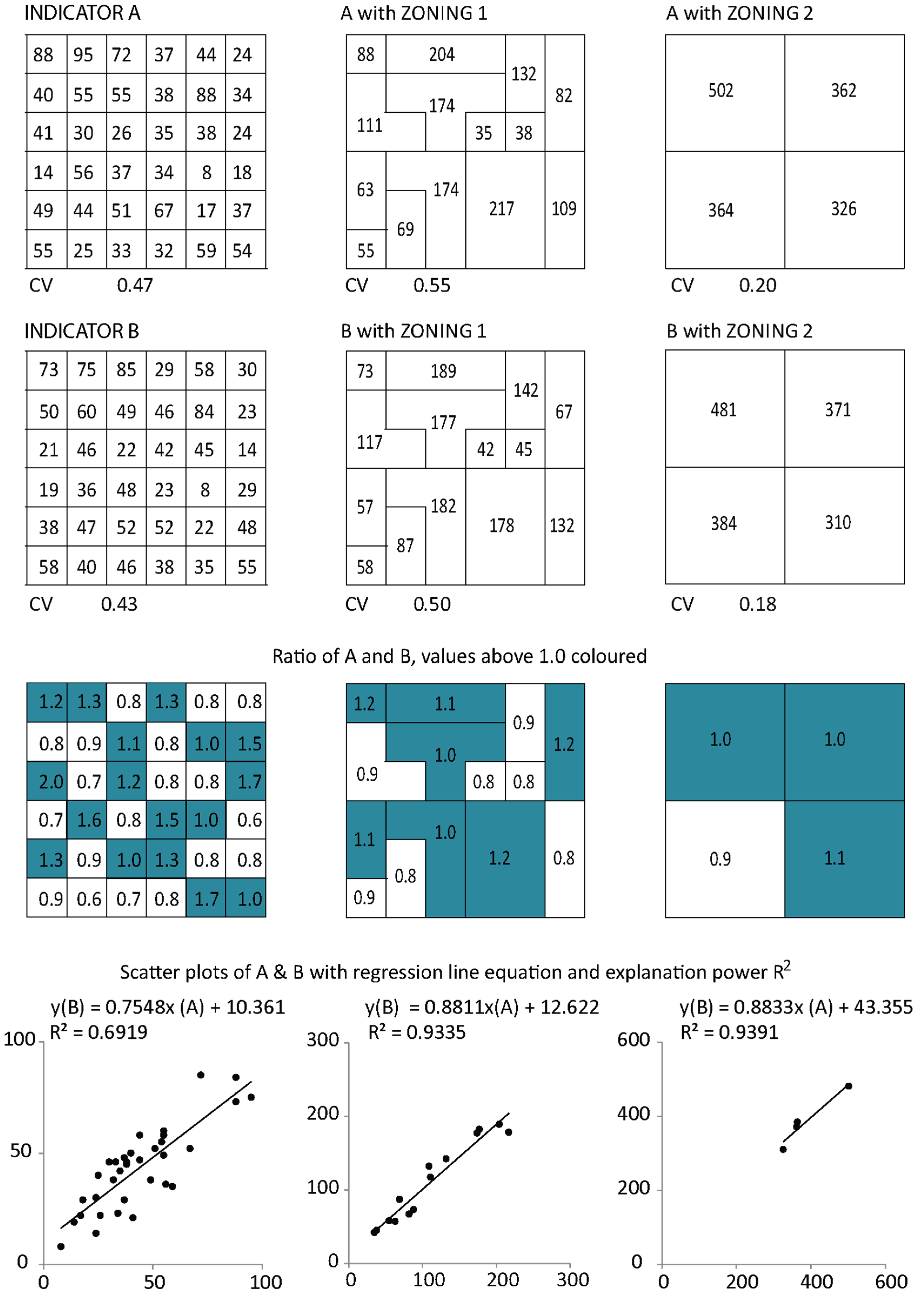
2. The Modifiable Areal Unit Problem (MAUP)

In an ideal world, data on the processes occurring on the surface of the Earth would be available with the same spatial resolution as the drivers influencing those processes [32]. Usually, however, different spatial resolutions are used, and this has a great impact on the results of the spatial analysis e.g., [32,50]. Two effects can be distinguished in the MAUP, one related to changing the scale or resolution of the data (scaling effect) and the other related to changing the criteria to divide the study area into units of analysis i.e., the zoning or aggregation scheme chosen for the study area (zoning effect). The latter is the focus of this study.
The scaling effect is observed when coarsening the spatial resolution (i.e., aggregating small areas into larger ones) and averaging the variables over each aggregation, which results in stronger correlation between the studied variables and the loss of degrees of freedom and variance [32,34,44]. Similarly, the zoning effect also causes differences in variance and correlation when comparing two different zonings of same data [44,51]. Relationships between variables can even switch from positive to negative when different units of analysis are used [44].
Figure 1 describes these basic ideas behind the MAUP. Two indicators, A and B, can be analyzed together with different zonings. The variables in the example could represent, for example, population and available water. The zoning effect is visible when looking at the change in the coefficient of variation (CV) and the explanatory power of regression (R2). When taking a ratio of the indicators A and B and exploring values above a certain threshold, we can see that results vary depending on the zoning used.
In practical terms, the MAUP thus means that statistical results are valid only at the spatial zoning and scale at which they were acquired [16,44,51,52,53]. This relates to the problem of ecological fallacy, which occurs if a researcher draws conclusions about a system on one scale based on results obtained at another scale (i.e., cross-scale inference) [32,54]. This phenomenon is particularly relevant since most policies and decisions are made at scales defined by administrative units, while data is often collected at other scales.
Figure 1. The basic idea of the Modifiable Areal Unit Problem (MAUP), partly based on [52]. A and B represent variables such as population and available water. In zoning 1, the units of analysis vary in size. In zoning 2, zones are created by regularly combining 9 grid cells.
Water 07 00898 g001

3. Materials and Methods
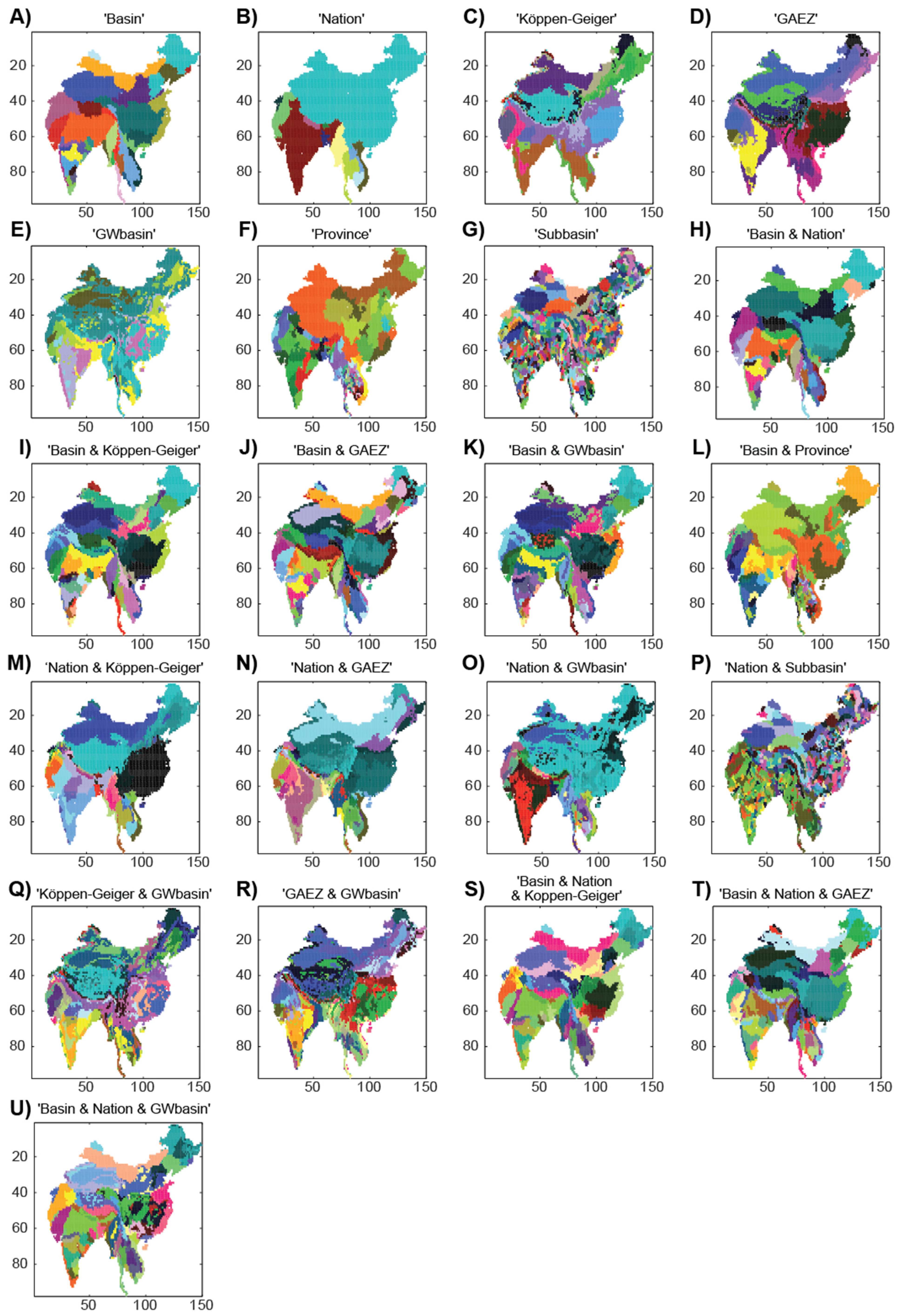
3.1. Zoning

There are two general approaches for zoning: (i) individual-level data can be classified into groups according to non-spatial information, such as socioeconomic status; or (ii) individual-level data can be organized based on location. In spatial assessment, the second way is natural, but there are an almost infinite number of ways to delineate boundaries to form regions [33]. There are also practical needs for dividing the study area in various ways, for example based on administrative boundaries or river basin boundaries, corresponding to the context or areas for which decisions and policies are typically made.
Traditionally, spatial units of analysis in water resources management have followed administrative boundaries, hydrological basins, or regular grid cells [17]. However, any region is characterized by a spectrum of social, cultural, physical, and economic factors, and it is not possible to claim that any of these traditional spatial units captures the spatial diversity of all these factors [55]. As a result, other spatial units are required as well.
This study used readily available data to define zonings and combinations of these (referred to as meshes). The data sources for calculating water shortage and for defining zoning schemes are presented in Table 1, together with the methods and preparations applied to these data. Data preparations were performed with R, ArcGIS 10.2 (ESRI, Redlands, CA, USA), and Matlab R2014a software (MathWorks, Natick, MA, USA) packages, while calculations were conducted and results were mapped with Matlab R2014a. Zonings and thus the units of analysis were varied such that both zoning and scaling effects of the MAUP could be studied. Figure 2 shows the variety of ways the study area was divided, consisting of seven baseline zonings (Figure 2A–G; Table 1), namely:
  • river basins (“Basin”) [56],
  • country boundaries (“Nation”) [57],
  • Köppen–Geiger climate zones (“Köppen–Geiger”) [58],
  • Global Agro-Ecological Zones (“GAEZ”) [59],
  • groundwater basins (“GWbasin”) [60],
  • province boundaries as one scale below from country boundaries (“Province”) [57] and finally
  • subbasins, defined as the scale below river basin boundaries (“Subbasin”) [56].
In addition, 14 meshes were created by combining two or three baseline division criteria (Figure 2H–U, Table 1).
Table 1. Summary of data & preparations.
Data for water shortageAverage annual runoff, 30 arc-minute resolution, source: WATCH 20th Century Ensemble [21,22].
Population (year 2010), 5 arc-minute, source: Grübler et al. [23] and Klein Goldewijk et al. [24].
Grid area, 30 arc-minute, source: HarvestChoice [61].
Water 07 00898 i001
Data for zoningsHydrological basins and subbasins: Hydrobasins [56].
Administrative boundaries: national and provincial level: GADM [57].
Köppen-Geiger Climate Zones [58].
Global Agro-ecological zones (GAEZ) [59].
Groundwater basins [60].
Zonings Water 07 00898 i002
Preparations in ArcGIS/RProjection was set to WGS84 (if not originally);
Data was converted to raster with ‘features to raster’ tool (if not originally), runoff raster was used as snap raster to ensure grid size and location was exactly the same for all rasters;
Grid cells were assigned numerical values representing zone codes;
Rasters were clipped according to the outer limits of the 10 major Asian river basins + including all river basins in China & India;
Rasters were converted to ASCII;
Average annual runoff was calculated in R based on the output of modelled daily surface and subsurface runoff for period of 1971–2000.
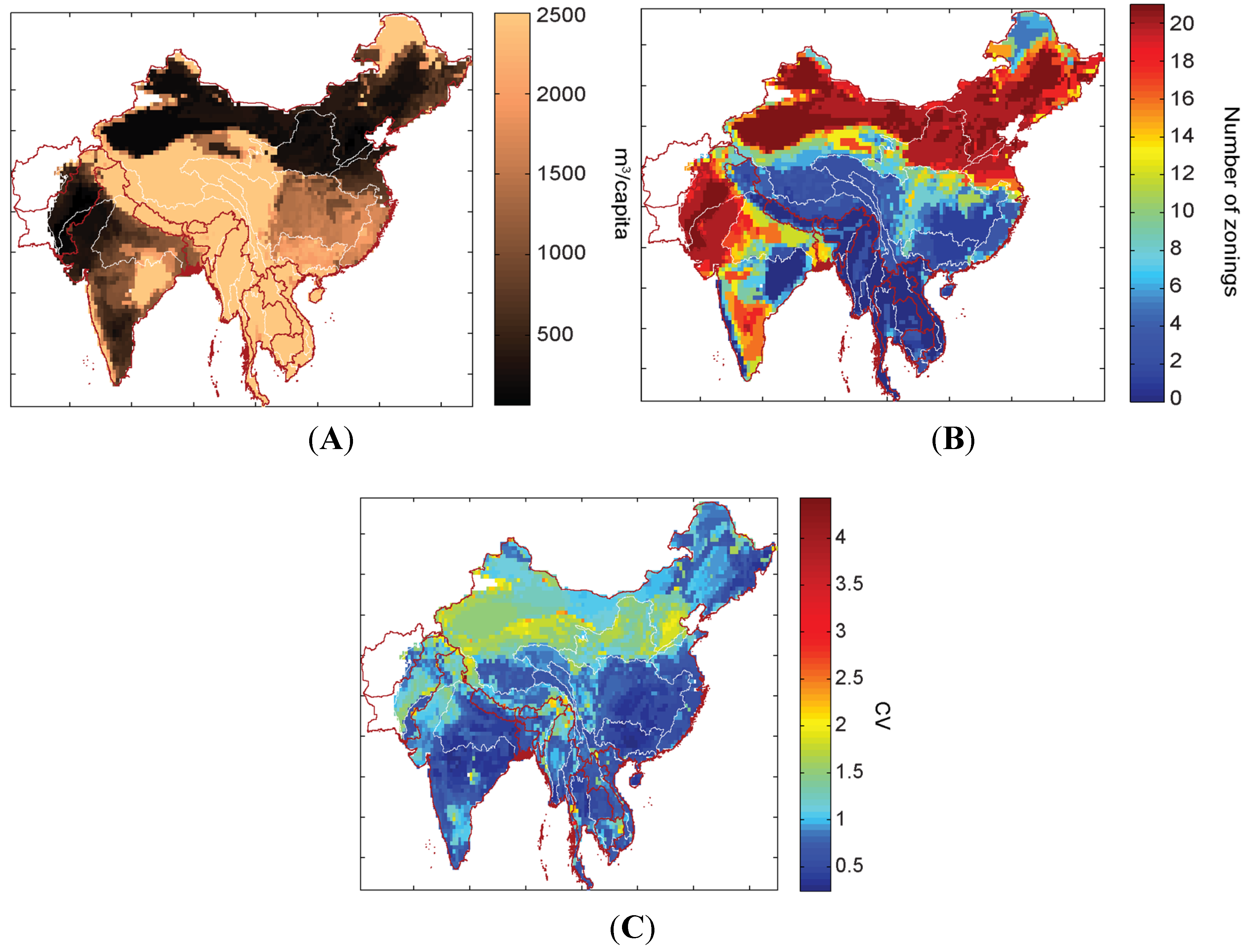
Preparations and calculations in MatlabPopulation for 2010 was calculated as combination of two 5 arc-minute datasets and aggregated to 30 arc-minute resolution;
Datasets were further clipped according to the minimum coverage of the input data, i.e., to consider only those grid cells that have values for all 21 zonings;
Meshes of zonings were created;
Zonal analysis was performed to calculate water availability, population and water shortage indicator for each zoning;
Water shortage indicator values assigned to each grid cell from each zoning were examined to calculate the average, standard deviation and coefficient of variation;
Population under 1000m3/cap/yr was calculated for each zoning;
The count of zonings when a grid cell fell under 1000m3/cap/yr was calculated;
Results were mapped and tabulated.
Figure 2. The 21 different zonings mapped. Data sources are presented in Table 1.
Water 07 00898 g002

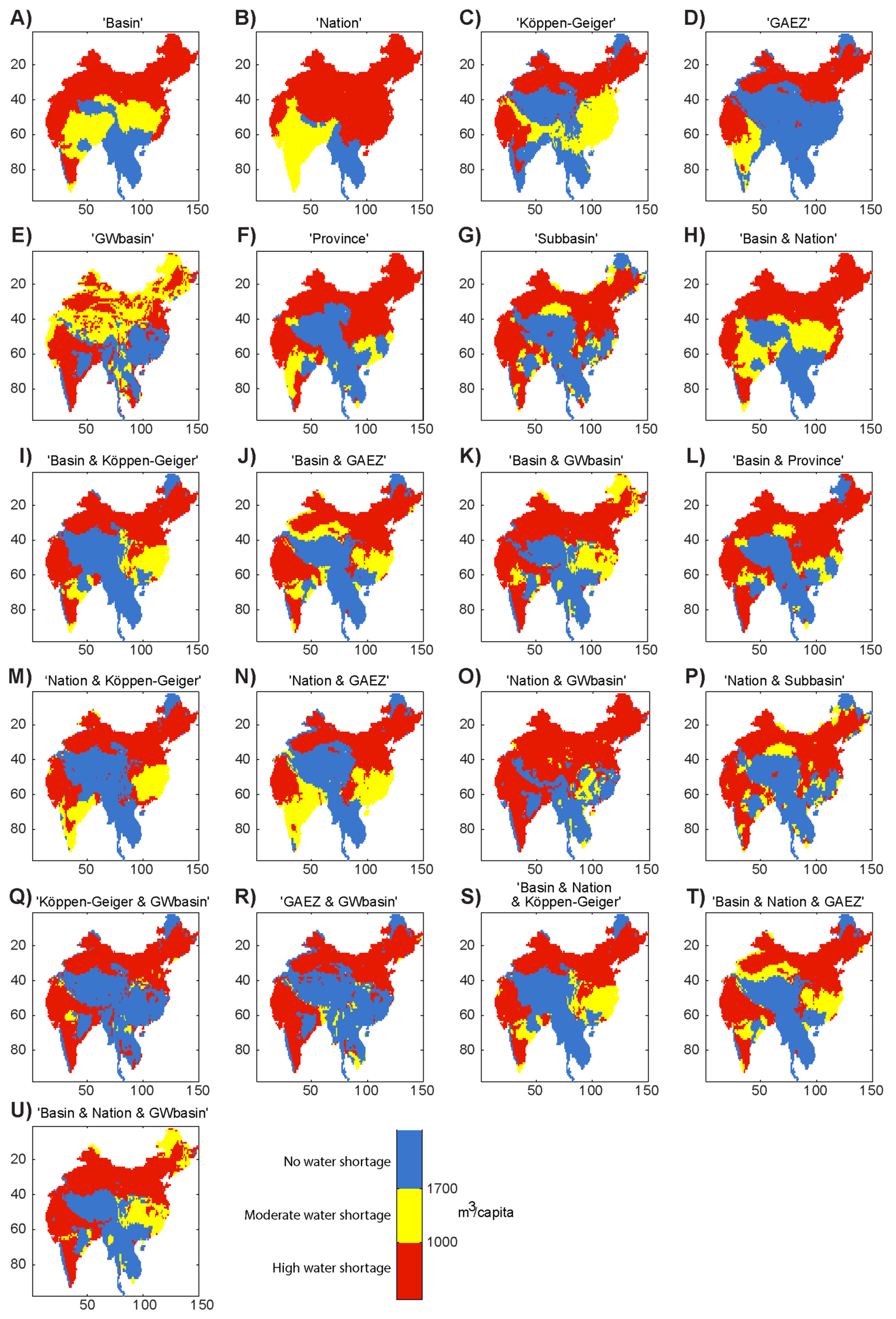
3.2. Water Shortage Calculations

The water shortage indicator is defined as the ratio of available water resources and population, measuring the average water availability per person in a unit of analysis [15,20,62]. We calculated water availability based on gridded mean annual runoff for the period 1971–2000 under natural conditions. The dataset was obtained at daily resolution from the WATCH project [21,22], which provides averaged total surface and sub-surface flow from seven global hydrological models. The dataset therefore represents a recent consensus regarding global runoff, particularly given that special care was taken to avoid bias due to outliers [21]. Daily values were aggregated to annual mean values. Grid-cell values were then multiplied with the surface area of the grid [61] using a resolution of 30 arc-minute (0.5°). We obtained population distribution data for 2010 by combining the datasets by Grübler et al. [23] and Klein Goldewijk et al. [24]. The original resolution of 5 arc-minutes was aggregated to 30 arc-minute resolution to fit with the other data.
Population and water availability were then aggregated to the areal units of analysis defined by the 21 zonings. Water shortage was calculated by dividing the available water in an areal unit of analysis by its population. For each zoning, we then calculated the total population under high water shortage, i.e., where the water availability is less than 1000 m3/cap/year in line with [27]. In addition, we calculated the average value of the water shortage indicator for each grid cell, based on the values from 21 different zonings. Finally, we calculated the variation of these values within each grid cell. The number of zonings in which the grid cell fell under high water shortage was recorded.

4. Results

Our results indicated that the spatial distribution of water shortage (Figure 3A–U) as well as the population under high water shortage (Table 2) varied considerably depending on the zoning used. The differences were easy to spot when water shortage indicator values were coarsely classified into “no”, “moderate”, and “high” water shortage (Figure 3).
Of the seven baseline zonings (Figure 3A–G), those based on groundwater aquifers and national boundaries (Figure 3E,B) produced quite different results (cf. Figure 3A–U). However, the province zoning, which is a “down-scaling” of the national zoning (Figure 3F), showed very similar patterns to most of the other zonings. The dataset on groundwater aquifers consists of areas that have been classified to represent aquifer types, and thus in theory a class can include groundwater aquifers that seem to be one continuous aquifer but in reality are not. Examination of the GW basin dataset together with, for example, national boundaries implied a more likely scenario where access to water is limited by access to a shared groundwater resource as well as national regulations. In such a case, the area under high water shortage increased remarkably (cf. Figure 3E,O).
Most of the areas under high water shortage in Figure 3E,O were major groundwater aquifers or aquifers with complex hydrogeological structure and recharge less than 100 mm/year [56]. Groundwater aquifers under high water shortage within Pakistan and China are classified as major groundwater basins with a recharge of less than 2 mm/year [60]. The water availability data includes surface and sub-surface (i.e., base flow from groundwater) runoff [21,22], but not fossil or unsustainably used groundwater resources. In many parts of the study area, groundwater is the main source of irrigation water (e.g., in India and Bangladesh [63,64] and in northern China [65,66]). This water shortage result therefore indicated that these regions are in fact dependent on that groundwater [63,64,65,66,67]. This is a significant result and supports the findings of Wada et al. [67].
Figure 3. Water shortage expressed in terms of available water resources per capita (m3/cap/year) with different zonings.
Water 07 00898 g003
Table 2. Population under high water shortage (water availability <1000 m3/cap/year) per each zoning.
ZoningPopulation Under High Water Shortage (in Billions)% of Total Population (~3.52 Billion)
1“Basin”1.2435%
2“Nation”1.4541%
3“Köppen–Geiger”0.7822%(min)
4“GAEZ”0.9527%
5“GWbasin”1.9756%
6“Province”1.9355%
7“Subbasin”2.1160%(max)
8“Basin & Nation”1.3538%
9“Basin & Köppen–Geiger”1.5544%
10“Basin & GAEZ”1.7650%
11“Basin & GWbasin”1.9656%
12“Basin & Province”2.0658%
13“Nation & Köppen–Geiger”1.3940%
14“Nation & GAEZ”1.2034%
15“Nation & GWbasin”2.0859%
16“Nation & Subbasin”2.0658%
17“Köppen–Geiger & GWbasin”2.0558%
18“GAEZ & GWbasin”1.8954%
19“Basin & Nation & Köppen–Geiger”1.5544%
20“Basin & Nation & GAEZ”1.8753%
21“Basin & Nation & GWbasin”2.0057%
Population under high water shortage also showed substantial variation. The results with different zonings ranged between 782 million (22% of total population) with the Köppen–Geiger climate zoning and 2.11 billion people (60% of total population) with subbasins as the unit of analysis (Table 2). The difference between these two extremes was almost a factor of three. Twelve out of 21 zonings resulted in population under high water shortage exceeding half of the total population, i.e., between 1.76 and 2.11 billion.
While our main aim was to study the zoning effect of the MAUP, the scaling effect was also clearly visible in our results. This is shown when comparing nations and provinces, and basins and subbasins, in both of which the former is a direct aggregation of the latter. In both cases, coarser resolution (higher scale) produced lower values. This is explained by the fact that averaging over larger areas reduces the effect of local concentrations of high population and low availability of water resources. The finer resolution zoning is more strongly affected by potential pockets of water shortage. In the case of basins and subbasins, the difference was 860 million and in the case of nations and provinces the difference was 480 million (Table 2). When comparing Figure 3A vs. Figure 3G and Figure 3B vs. Figure 3F, the number of grid cells under high water shortage was actually higher when using a coarser scale, but the subbasin and province scales produced a larger population under high water shortage because of the high population density in the cells affected, particularly in Bangladesh and in the parts of India within the Ganges-Brahmaputra-Meghna region.
The coefficient of variation (CV) was calculated for each grid cell of 30 arc-minute (21 values each, corresponding to the zonings). The CV revealed that the variation in water shortage was greatest in the areas with lowest average water shortage (cf. Figure 4A,B).
Figure 4. (A) Average water shortage per grid cell calculated based on the 21 zonings; (B) number of zonings under which the water shortage indicator value for grid cell was less than 1000 m3/cap/year; and (C) the coefficient of variation (CV) of water shortage indicator values per grid cell calculated over the 21 zonings.
Water 07 00898 g004
The groundwater aquifer zoning was likely to have caused some of this high variation, as its values differed the most from other zonings’ values, particularly in the northern parts of the study area (Figure 3E). The “GAEZ” and “Köppen–Geiger” zonings also produced somewhat different shortage maps (Figure 3C,D). On the other hand, the overall view of Figure 4A–C reveals that areas with lowest average water availability per capita were located in areas which also tend to be categorized as areas under high water shortage with the majority of the zonings (>17, Figure 4C).
Examples of areas that were particularly prone to the MAUP are parts of China with a high average water availability, i.e., over 1700 m3/cap/year (Figure 4A, lighter color). However, these areas were classified as areas under high water shortage in roughly half of the zonings (Figure 3 and Figure 4B, light blue and green areas) and received high CV values (Figure 4C). In these areas, groundwater use might already be unsustainable [63,66,67], which makes the uncertainty of water shortage even more problematic.
While the different zonings brought remarkable heterogeneity to the results, there were commonalities across all zonings: (i) the areas within the Indus River basin in the western part of the study area; (ii) the northern part of the study area including the Yellow River Basin; (iii) the northwest part of China; and (iv) the northwest part of India (Figure 3 and Figure 4A,B).

5. Discussion

The study revealed that different zonings used in our spatial assessment resulted in substantial variation in water shortage results. In particular, the spatial extent and population under high water shortage (<1000 m3/cap/year) vary remarkably depending on the zoning used. The significant effect of scale was also visible in our results, in line with the findings of Vörösmarty et al. [9] and Perveen and James [15]. In general, when using more detailed data (grid-based), the population under scarcity increases compared with coarser data (e.g., national statistics) [9].
The values of the water shortage indicator varied substantially in areas with low average water availability, but also in areas that experienced high water shortage in half the zonings while still having higher average water availability. This indicates a high level of sensitivity to and importance of the selection of the areal unit of analysis. Despite the substantial variation in the results, the areas most affected by annual water shortage were still visible and were classified as high water shortage according to 17 or more zonings. These were found in areas within the Indus River basin, the Yellow River basin, and the northwest parts of India and China (Figure 4A,B).
We used some of the most recent runoff and population datasets available, and thus extended previous work, e.g., the water stress analysis by Vörösmarty et al. [4]. We considered not just grid cells that have river flow, but also sub-surface runoff and the zoning associated with groundwater aquifers. This study thus provided support for findings of other relevant studies on water scarcity regarding groundwater-related aspects [63,68,69,70] as well as new findings.
To our knowledge this analysis was the first to look systematically at the MAUP’s zoning effect—in a water scarcity context—for a large study area covering several countries and major river basins. The study provides issues to consider when conducting national-, regional-, or global-scale spatial assessments related to water resources. We have shown that the MAUP has such a dramatic effect on estimates of water shortage that it is essential that this issue be explicitly tackled by anybody using these assessments e.g., for policy analysis. The ability of the spatial data user to modify the areal unit of analysis and hence to influence analysis results comes with great responsibility.
In the remainder of the discussion, we consider how spatial data users may be able to meet this responsibility. We first discuss whether it is possible to robustly estimate the water shortage indicator. This would be the ideal outcome; what is the value of an indicator if its message can be too easily modified? We then discuss factors that need to be considered in estimating water shortage, including the role of the zones used in this paper. We conclude with recommendations for the best way forward.

5.1. Can We Solve the MAUP to Robustly Estimate the Water Shortage Indicator?

Ideally, the water shortage indicator would be calculated based on the volume of water to which individuals actually have access compared to the volume of water they require. There is, in principle, a right answer when quantifying the water shortage. This suggests that improved access to detailed data about access and demand for water would be one way to avoid the MAUP. However, collecting data at such a detailed level is practically impossible due to cost and confidentiality issues [71], hence the need to use spatially aggregated statistics. In addition, the drivers affecting the use and management of water resources can also operate at larger scales, and using the most detailed level of data may not always be appropriate [16], even if it were accessible. Drivers typically depend on scale and the relevance of drivers at different scales therefore varies.
Using spatially aggregated data means that the MAUP cannot be fully avoided, and the aim should thus be to recognize and minimize its effects. The magnitude of the MAUP is influenced by the variation among the observations and by the extent to which the unit of analysis matches this pattern [33]. The MAUP is therefore related to the internal homogeneity of areal units, and in this way also to spatial autocorrelation [54] and to the first law of geography stating that “near things are more related than distant things” [72]. This suggests that the optimal areal unit of analysis could be formed based on the degree of auto-correlation (by variogram, semivariogram, or correlogram) or by other data-driven methods such as the k-means clustering.
An example of optimizing the unit of analysis can be drawn from a case study of the Tonle Sap Lake in Cambodia [73], in which socioeconomic data were clustered spatially instead of according to provincial boundaries, enabling exploration of areas with similar linkages between economic activity and the lake’s hydrology. The study concluded that optimizing the unit of analysis to consider these local characteristics enables further discussion of potential impacts of changes in the lake’s hydrology on livelihoods.
In the above example, however, the MAUP is not actually “solved.” While its effects are minimized from the viewpoint of the case study, there are other viewpoints that would lead to different “optimal” units of analysis and the same data could reveal different results. Thus, it seems that attempts to minimize the effects of the MAUP are strongly case-specific and location-specific.

5.2. Factors to Consider in Estimating Water Shortage

In this study different assumptions about availability, access, and demand relating to water were considered through the use of multiple zonings. Each zoning reflects the inability to obtain water (or goods produced using water) for a particular population from other basins, nations, climate zones, agro-ecological zones, groundwater basins, subbasins, provinces, or combinations of these. In other words, when calculating water shortage indicator, we assume that there are distinct areas within which the population is limited to using only water from the same area. This touches on a number of considerations.
The groundwater aquifers provided a striking example, where access to water is limited to a shared groundwater resource (resulting in 56% of population under high water shortage, 59% if access is also limited within national boundaries, Table 2). High shortage of surface and sub-surface runoff in these areas suggested a dependence on fossil groundwater. Virtual (or physical) water imports from other parts of a nation (i.e., using national boundaries) can reduce water shortage (41% under high water shortage), but may not be possible due to problems interacting between provinces (55%). Use of river flows or virtual water imports from outside the nation (e.g., within river basin boundaries 35%) may require significant transboundary negotiation or imply a loss of food sovereignty. Boundaries associated with climate zones and agro-ecological zones can be interpreted as implying unlimited trade of goods produced while relying on runoff of the local climate (22%) or minimizing the use of runoff outside its original agro-ecological zone (27%). These seem like more utopian scenarios, assuming that the benefits of water are being equitably distributed among all people within a region. The other extreme occurs if people are restricted to the runoff within their subbasin (60%), as may be the case in headwaters reliant on subsistence agriculture.
Additional factors could be considered in optimizing the unit of analysis to avoid the MAUP. A number of limitations of the indicator have been reported e.g., [14,19,63]. Heterogeneity of water demand and seasonal variation in both water availability and demand could be addressed. Furthermore, it would be useful to extend the analysis beyond physical water availability to consideration of water quality, resource management, and social and economic factors limiting water access, including their variation over time. However, detailed and location-specific data on water availability and demand with specific information on diet, water use, and resource management are not currently available. Without this information, calculation of water shortage at a detailed level is not possible. For example, calculating the water availability of an urban area requires information about connections to its vast hinterland. Otherwise, a single isolated urban grid cell would appear to have high water shortage, where it may not actually be the case.
This complexity of factors influencing water shortage suggests that zonings should instead be seen as purpose-dependent. The definitions of available water and of needs are intrinsically subjective. In theory, water that is considered to be available to a population could range from only the water in a grid cell to potentially all the water in the world, making use of the virtual water concept [74]. Ultimately, while the individual consumer may be able to determine whether their needs are met at a point in time, it should be noted that different sectors would probably have very different opinions of optimal and relevant scales and zonings. The amount of water needed to avoid shortage can range from basic needs for drinking water to the water demand of an agricultural industry dependent on irrigation in a climate region otherwise not suitable for crop production. Food production involving supply chains would have quite a different view on the optimal unit of analysis to calculate the water shortage compared with the energy sector. Each of these perspectives corresponds to different purposes of analysis and yields different zonings and results. The same issue was discussed previously in the context of the Tonle Sap case study. It is obviously important that the purpose of the analysis and the reasoning behind the unit of analysis are transparently reported and discussed.

5.3. A Way Forward

Given the challenges described above, it seems fair to say that the MAUP is here to stay. While some methods have been developed for quantifying the MAUP and handling its influence [41,51,55,75,76,77,78,79,80], none of these methods provides a comprehensive solution that would easily quantify the effect of the MAUP [34] or enable finding consistent results regardless of the scale or zonal patterns [33]. Therefore, our results also reinforce the findings of previous studies [15,16,17], noting that multizonal and multiscale approaches are required for spatial assessments. Such approaches are important as they reveal the sensitivity of the results to the selection of the unit of analysis and data resolution, and increase the robustness of conclusions drawn from the results. A multizonal approach enables a sensitivity analysis for indicator-based assessments, regarding the spatial dimension. Using multiple zones can also be an effective way of representing multiple perspectives, facilitating dialogue between different sectors.
However, there are also issues that need to be considered with multizonal and multiscale assessments. There is a danger of overstating uncertainty by including zonings that are not strongly representative of the issue in hand. Using too many different zonings may also overload the audience with unnecessarily detailed information. If fewer zonings are used, new research is still needed to evaluate whether sufficiently different zonings are included. The selection of zones therefore needs to be considered critically to ensure extensive coverage of various viewpoints, rather than simply using all zones available. It is also important to explicitly discuss how the recommendations might change if different assumptions were made and different zones were selected.

6. Conclusions

We addressed the Modifiable Areal Unit Problem (MAUP) in spatial water shortage assessment by systematically exploring the impact that the unit of analysis and zoning system have on the results. This was done using 21 different criteria for defining the unit of analysis within a study area covering Monsoon Asia.
Our results revealed that the spatial extent and population under high water shortage (<1000 m3/cap/year) varied remarkably depending on the zoning used. Our findings also allowed us to identify the areas with the highest frequency of water shortage among the various zonings, namely the areas within the Indus and the Yellow River basins and areas in the northwestern parts of India and China. While nearly all zonings resulted in high water shortage in these areas, the value of the water shortage indicator also varied most in those areas, especially close to these areas where average water availability was higher. This indicates a high level of sensitivity to the selection of the unit of analysis.
Our analysis reinforces the view that results of spatial studies are sensitive to the zoning system used. This means that the selection of the scale and the areal units of analysis cannot be considered an independent and neutral part of the spatial assessment, as it may have a major influence on assessment results. Hence, as a first practical step, it is important that the scale and unit of analysis used are transparently described and their possible effects on the results are openly discussed as part of any spatial assessment. A further step forward is to simultaneously use several scales and units of analysis and to discuss their differences consistently and openly. Only this kind of multiscale and multizonal assessment approach can make the challenges of the MAUP and its scaling and zoning effects properly visible.
At the theoretical level, this problem has long been recognized [31], but we argue that it needs to be more consistently used and understood in interpreting and discussing outcomes of water-resources related spatial analyses. We hope that our analysis and findings—showing that remarkable variation in water shortage results stems from the selection of the unit of analysis—will inspire scientists as well as the users of the spatial assessment results to go beyond debating the numbers to debating the factors behind the numbers.

Acknowledgments

The authors are grateful for the WHYMAP team at BGR and UNESCO for sharing the groundwater basin dataset for our analysis. The two anonymous reviewers are thanked for their excellent comments and suggestions that contributed to improving the article. The authors would also like to thank their colleagues at Aalto University’s Water & Environmental Engineering Research Group for their support. Aura Salmivaara received funding from the VALUE Doctoral School, Aalto University Fund, the Academy of Finland project 133748, and the Academy of Finland project 269901. Miina Porkka received funding from Maa- ja vesitekniikan tuki ry. Matti Kummu received funding from the Academy of Finland funded project SCART (grant No. 267463). Marko Keskinen received funding from the Academy of Finland project 269901. Olli Varis received funding from the Finnish Cultural Foundation.

Author Contributions

Aura Salmivaara designed the study, gathered the data used for the assessment, and performed the analyses. Aura Salmivaara prepared figures and was responsible for writing the manuscript. Miina Porkka, Matti Kummu, and Joseph H. A. Guillaume participated in designing the study, gathering the data used, and assisting with the analyses. Aura Salmivaara, Miina Porkka, Matti Kummu, and Joseph H. A. Guillaume jointly discussed the results. Aura Salmivaara, Matti Kummu, Miina Porkka, Marko Keskinen, Joseph H. A. Guillaume, and Olli Varis all contributed in further discussion of the results and in editing and refining the manuscript.

Conflicts of Interest

The authors declare no conflict of interest.

References

  1. Eade, J.D.O.; Moran, D. Spatial economic valuation: Benefits transfer using Geographical Information Systems. J. Environ. Manag. 1996, 48, 97–110. [Google Scholar] [CrossRef]
  2. Herr, A. Data integration issues in research supporting sustainable natural resource management. Geogr. Res. 2007, 45, 376–386. [Google Scholar] [CrossRef]
  3. Van Oel, P.R.; Odongo, V.O.; Mulatu, D.W.; Muthoni, F.K.; Ndungu, J.N.; Ogada, J.O.; van der Veen, A. Supporting IWRM through spatial integrated assessment in the Lake Naivasha basin, Kenya. Int. J. Water Resour. Dev. 2014, 30, 605–618. [Google Scholar] [CrossRef]
  4. Vörösmarty, C.J.; McIntyre, P.B.; Gessner, M.O.; Dudgeon, D.; Prusevich, A.; Green, P.; Glidden, S.; Bunn, S.E.; Sullivan, C.A.; Liermann, C.R.; et al. Global threats to human water security and river biodiversity. Nature 2010, 467, 555–561. [Google Scholar] [CrossRef] [PubMed]
  5. Del Campo, A.G. GIS in environmental assessment: A review of current issues and future needs. J. Environ. Assess. Policy Manag. 2012, 14. [Google Scholar] [CrossRef]
  6. Chapman, L.; Thornes, J.E. The use of Geographical Information Systems in climatology and meteorology. Progress Phys. Geogr. 2003, 27, 313–330. [Google Scholar] [CrossRef]
  7. Díez, E.; McIntosh, B.S. A review of the factors which influence the use and usefulness of information systems. Environ. Model. Softw. 2009, 24, 588–602. [Google Scholar] [CrossRef]
  8. Volk, M.; Lautenbach, S.; van Delden, H.; Newham, L.T.; Seppelt, R. How can we make progress with decision support systems in landscape and river basin management? Lessons learned from a comparative analysis of four different decision support systems. Environ. Manag. 2010, 46, 834–849. [Google Scholar] [CrossRef]
  9. Vörösmarty, C.J.; Green, P.; Salisbury, J.; Lammers, R.B. Global water resources: Vulnerability from climate change and population growth. Science 2000, 289, 284–288. [Google Scholar] [CrossRef] [PubMed]
  10. Kummu, M.; de Moel, H.; Eisner, S.; Flörke, M.; Guillaume, J.H.A.; Porkka, M.; Siebert, S.; Veldkamp, T.I.E.; Ward, P.J. Global water use and water scarcity trajectories for the 20th century. Available online: http://meetingorganizer.copernicus.org/EGU2014/EGU2014-12310.pdf (accessed on 28 February 2015).
  11. Schewe, J.; Heinke, J.; Gerten, D.; Haddeland, I.; Arnell, N.W.; Clark, D.B.; Dankers, R.; Eisner, S.; Fekete, B.M.; Colón-González, F.J.; et al. Multimodel assessment of water scarcity under climate change. Proc. Natl. Acad. Sci. USA 2014, 111, 3245–3250. [Google Scholar] [CrossRef] [PubMed] [Green Version]
  12. Varis, O.; Kummu, M.; Salmivaara, A. Ten major river basins in Monsoon Asia-Pacific: An assessment of vulnerability. Appl. Geogr. 2012, 32, 441–454. [Google Scholar] [CrossRef]
  13. UN DESA. World Population Prospects: The 2012 revision. Population Division of the Department of Economic and Social Affairs of the United Nations Secretariat. Available online: http://esa.un.org/unpd/wpp/index.htm (accessed on 21 August 2014).
  14. Rockström, J.; Falkenmark, M.; Karlberg, L.; Hoff, H.; Rost, S.; Gerten, D. Future water availability for global food production: The potential of green water for increasing resilience to global change. Water Resour. Res. 2009, 45. [Google Scholar] [CrossRef]
  15. Perveen, S.; James, L.A. Scale invariance of water stress and scarcity indicators: Facilitating cross-scale comparisons of water resources vulnerability. Appl. Geogr. 2011, 31, 321–328. [Google Scholar] [CrossRef]
  16. Perveen, S.; James, L.A. Changes in correlation coefficients with spatial scale and implications for water resources and vulnerability data. Prof. Geogr. 2012, 64, 389–400. [Google Scholar] [CrossRef]
  17. Perveen, S.; James, L.A. Multiscale effects on spatial variability metrics in global water resources data. Water Resour. Manag. 2010, 24, 1903–1924. [Google Scholar] [CrossRef]
  18. Brown, A.; Matlock, M.D. A review of water scarcity indices and methodologies. Available online: http://www.sustainabilityconsortium.org/wp-content/themes/sustainability/assets/pdf/whitepapers/2011_Brown_Matlock_Water-Availability-Assessment-Indices-and-Methodologies-Lit-Review.pdf (accessed on 10 June 2014).
  19. Rijsberman, F.R. Water scarcity: Fact or fiction? Agric. Water Manag. 2006, 80, 5–22. [Google Scholar] [CrossRef]
  20. Falkenmark, M.; Lundqvist, J.; Widstrand, C. Macro-scale water scarcity requires micro-scale approaches. Aspects of vulnerability in semi-arid development. Natl. Resour. Forum 1989, 13, 258–267. [Google Scholar] [CrossRef]
  21. Weedon, G. Watch Technical Report Number 37, Creation of the Watch 20th Century Ensemble Product; Technical Report. UK Met Office: Wallingford, UK, 2011. Available online: http://www.eu-watch.org/media/default.aspx/emma/org/10730457/Technical+Report+37+Creation+of+the+WATCH+20th+Century+Ensemble+Product.pdf (accessed on 18 January 2015).
  22. Haddeland, I.; Clark, D.B.; Franssen, W.; Ludwig, F.; Voß, F.; Arnell, N.W.; Bertrand, N.; Best, M.; Folwell, S.; Gerten, D. Multimodel estimate of the global terrestrial water balance: Setup and first results. J. Hydrometeorol. 2011, 12, 869–884. [Google Scholar] [CrossRef]
  23. Grübler, A.; O’Neill, B.; Riahi, K.; Chirkov, V.; Goujon, A.; Kolp, P.; Prommer, I.; Scherbov, S.; Slentoe, E. Regional, national, and spatially explicit scenarios of demographic and economic change based on SRES. Technol. Forecast. Soc. Chang. 2007, 74, 980–1029. [Google Scholar] [CrossRef]
  24. Klein Goldewijk, K.; Beusen, A.; Janssen, P. Long-term dynamic modelling of global population and built-up area in a spatially explicit way: HYDE 3.1. Holocene 2010, 20, 565–573. [Google Scholar] [CrossRef]
  25. Gassert, F.; Reig, P.; Luo, T.; Maddocks, A. Aqueduct Country and River Basin Rankings: A Weighted Aggregation of Spatially Distinct Hydrological Indicators, Working Paper; World Resources Institute: Washington, DC, USA, 2013. [Google Scholar]
  26. Arnell, N.W. Climate change and global water resources: SRES emissions and socio-economic scenarios. Glob. Environ. Chang. 2004, 14, 31–52. [Google Scholar] [CrossRef]
  27. Kummu, M.; Ward, P.J.; de Moel, H.; Varis, O. Is physical water scarcity a new phenomenon? Global assessment of water shortage over the last two millennia. Environ. Res. Lett. 2010, 5. [Google Scholar] [CrossRef]
  28. Meybeck, M.; Kummu, M.; Dürr, H.H. Global hydrobelts and hydroregions: Improved reporting scale for water-related issues? Hydrol. Earth Syst. Sci. 2013, 17, 1093–1111. [Google Scholar] [CrossRef]
  29. Oki, T.; Agata, Y.; Kanae, S.; Saruhashi, T.; Yang, D.; Musiake, K. Global assessment of current water resources using total runoff integrating pathways. Hydrol. Sci. J. 2001, 46, 983–995. [Google Scholar] [CrossRef]
  30. Arnell, N.W.; van Vuuren, D.P.; Isaac, M. The implications of climate policy for the impacts of climate change on global water resources. Glob. Environ. Chang. 2011, 21, 592–603. [Google Scholar] [CrossRef]
  31. Gain, A.K.; Giupponi, C.; Renaud, F.G. Climate change adaptation and vulnerability assessment of water resources systems in developing countries: A generalized framework and a feasibility study in Bangladesh. Water 2012, 4, 345–366. [Google Scholar] [CrossRef] [Green Version]
  32. Goodchild, M.F. Scale in GIS: An overview. Geomorphology 2011, 130, 5–9. [Google Scholar] [CrossRef]
  33. Wong, D.W. Modifiable Areal Unit Problem. In International Encyclopedia of Human Geography; Rob, K., Nigel, T., Eds.; Elsevier: Oxford, UK, 2009; pp. 169–174. [Google Scholar]
  34. Dark, S.J.; Bram, D. The Modifiable Areal Unit Problem (MAUP) in Physical Geography. Prog. Phys. Geogr. 2007, 31, 471–479. [Google Scholar] [CrossRef]
  35. Gehlke, C.E.; Biehl, K. Certain effects of grouping upon the size of the correlation coefficient in census tract material. J. Am. Stat. Assoc. 1934, 29, 169–170. [Google Scholar]
  36. Fotheringham, A.S.; Wong, D.W.S. The Modifiable Areal Unit Problem in multivariate statistical analysis. Environ. Plan. A 1991, 23, 1025–1044. [Google Scholar] [CrossRef]
  37. Goodchild, M.F.; Quattrochi, D.A. Scale, Multiscaling, Remote Sensing, and GIS; CRC Press LLC: Boca Raton, FL, USA, 1997. [Google Scholar]
  38. Amrhein, C.; Reynolds, H. Using spatial statistics to assess aggregation effects. Geogr. Syst. 1996, 3, 143–158. [Google Scholar]
  39. Arbia, G.; Benedetti, R.; Espa, G. Effects of the MAUP on image classification. Geogr. Syst. 1996, 3, 123–141. [Google Scholar]
  40. Marceau, D.J.; Gratton, D.J.; Fournier, R.A.; Fortin, J.-P. Remote sensing and the measurement of geographical entities in a forested environment. 2. The optimal spatial resolution. Remote Sens. Environ. 1994, 49, 105–117. [Google Scholar] [CrossRef]
  41. Openshaw, S. A geographical solution to scale and aggregation problems in region-building, partitioning and spatial modelling. Trans. Inst. Br. Geogr. 1977, 459–472. [Google Scholar] [CrossRef]
  42. Openshaw, S. Ecological fallacies and the analysis of areal census data. Environ. Plan. A 1984, 16, 17–31. [Google Scholar] [CrossRef] [PubMed]
  43. Openshaw, S.; Alvanides, S. Designing zoning system for the representation of socio-economic data. In Life and Motion of Socio-Economic Units, GISDATA 8 Series; Masser, I., Salgé, F., Frank, A., Raper, J., Cheylan, J.-P., Eds.; Taylor & Francis: London, UK, 2001; pp. 273–292. [Google Scholar]
  44. Openshaw, S.; Taylor, P.J. A million or so correlation coefficients: Three experiments on the Modifiable Areal Unit Problem. Stat. Appl. Spat. Sci. 1979, 21, 127–144. [Google Scholar]
  45. Kattelus, M.; Kummu, M.; Keskinen, M.; Salmivaara, A.; Varis, O. China’s south-bound transboundary river basins—A case of asymmetry. Water Int. 2015, 40, 113–138. [Google Scholar] [CrossRef]
  46. WWAP. The United Nations world water development report 2014: Water and energy. In United Nations World Water Assessment Programme; UNESCO: Paris, France, 2014. [Google Scholar]
  47. Lorenz, C.M.; Gilbert, A.J.; Cofino, W.P. Indicators for transboundary river management. Environ. Manag. 2001, 28, 115–129. [Google Scholar] [CrossRef]
  48. Gain, A.K.; Giupponi, C. A dynamic assessment of water scarcity risk in the lower Brahmaputra River basin: An integrated approach. Ecol. Indic. 2015, 48, 120–131. [Google Scholar] [CrossRef]
  49. Käkönen, M.; Hirsch, P. The anti-politics of Mekong knowledge production. In Contested Waterscapes in the Mekong Region-Hydropower, Livelihoods and Governance; Molle, F., Foran, T., Käkönen, M., Eds.; Earthscan: London, UK; Sterling, VA, USA, 2009. [Google Scholar]
  50. Mandelbrot, B.B. How long is the coast of Britain. Science 1967, 156, 636–638. [Google Scholar] [CrossRef] [PubMed]
  51. Openshaw, S. The Modifiable Areal Unit Problem; Geo Books: Norwich, UK, 1983. [Google Scholar]
  52. O’Sullivan, D.; Unwin, D.J. The pitfalls and potential of spatial data. In Geographic Information Analysis; John Wiley & Sons, Inc.: Hoboken, NJ, USA, 2010; pp. 33–53. [Google Scholar]
  53. Clark, W.A.; Avery, K.L. The effects of data aggregation in statistical analysis. Geogr. Anal. 1976, 8, 428–438. [Google Scholar] [CrossRef]
  54. King, G. A Solution to the Ecological Inference Problem: Reconstructing Individual Behavior from Aggregate Data; Princeton University Press: Princeton, NJ, USA, 2013. [Google Scholar]
  55. Nelson, A. Analysing data across geographic scales in Honduras: Detecting levels of organisation within systems. Agric. Ecosyst. Environ. 2001, 85, 107–131. [Google Scholar] [CrossRef]
  56. Lehner, B.; Verdin, K.; Jarvis, A. New global hydrography derived from spaceborne elevation data. Eos Trans. AGU 2008, 89, 93–94. [Google Scholar] [CrossRef]
  57. GADM Database for Global Administrative Areas, version 2.0. Available online: www.gadm.org (accessed on 24 March 2014).
  58. Kottek, M.; Grieser, J.; Beck, C.; Rudolf, B.; Rubel, F. World map of the Köppen-Geiger climate classification updated. Meteorol. Z. 2006, 15, 259–263. [Google Scholar] [CrossRef]
  59. Ramankutty, N.; Hertel, T.; Lee, H.-L.; Rose, S.K. Global agricultural land use data for integrated assessment modelling. In Human-Induced Climate Change—An Interdisciplinary Assessment; Schlesinger, M.E., Kheshgi, H.S., Smith, J., de la Chesnaye, F.C., Reilly, J.M., Wilson, T., Kolstad, C., Eds.; Cambridge University Press: Cambridge, UK, 2007. [Google Scholar]
  60. BGR & UNESCO. Groundwater resources of the world 1:25,000,000. Hannover: Germany, Paris, France. Available online: http://www.whymap.org (accessed on 1 April 2014).
  61. HarvestChoice. HCID: Grid databases at multiple spatial resolutions. Available online: http://harvestchoice.org/node/2232 (accessed on 24 April 2014).
  62. Falkenmark, M.; Widstrand, C. Population and water resources: A delicate balance. Popul. Bull. 1992, 47, 1–36. [Google Scholar] [PubMed]
  63. Shah, T.; Singh, O.P.; Mukherji, A. Some aspects of South Asia’s groundwater irrigation economy: Analyses from a survey in India, Pakistan, Nepal Terai and Bangladesh. Hydrogeol. J. 2006, 14, 286–309. [Google Scholar] [CrossRef]
  64. Shahid, S.; Behrawan, H. Drought risk assessment in the western part of Bangladesh. Nat. Hazards 2008, 46, 391–413. [Google Scholar] [CrossRef]
  65. Siebert, S.; Burke, J.; Faures, J.-M.; Frenken, K.; Hoogeveen, J.; Döll, P.; Portmann, F.T. Groundwater use for irrigation—A global inventory. Hydrol. Earth Syst. Sci. 2010, 14, 1863–1880. [Google Scholar]
  66. Wang, J.; Huang, J.; Blanke, A.; Huang, Q.; Rozelle, S. The development, challenges and management of groundwater in rural China. In The Agricultural Groundwater Revolution: Opportunities and Threats to Development; Giordano, M., Villholt, K.G., Eds.; International Water Management Institute: Colombo, Sri Lanka; CAB International: Wallingford, UK, 2007; pp. 37–62. [Google Scholar]
  67. Wada, Y.; Bierkens, M.F.P. Sustainability of global water use: Past reconstruction and future projections. Environ. Res. Lett. 2014, 9. [Google Scholar] [CrossRef]
  68. Gleeson, T.; Wada, Y.; Bierkens, M.F.P.; van Beek, L.P.H. Water balance of global aquifers revealed by groundwater footprint. Nature 2012, 488, 197–200. [Google Scholar] [CrossRef] [PubMed]
  69. Wada, Y.; van Beek, L.P.H.; Bierkens, M.F.P. Nonsustainable groundwater sustaining irrigation: A global assessment. Water Resour. Res. 2012, 48. [Google Scholar] [CrossRef]
  70. Wada, Y.; van Beek, L.P.H.; van Kempen, C.M.; Reckman, J.W.T.M.; Vasak, S.; Bierkens, M.F.P. Global depletion of groundwater resources. Geophys. Res. Lett. 2010, 37. [Google Scholar] [CrossRef]
  71. Weeks, J.R. The role of spatial analysis in demographic research. In Spatially Integrated Social Science; Goodchild, M.F., Janelle, D.G., Eds.; Oxford University Press: Oxford, UK, 2004; pp. 381–399. [Google Scholar]
  72. Tobler, W.R. A computer movie simulating urban growth in the Detroit region. Econ. Geogr. 1970, 46, 234–240. [Google Scholar] [CrossRef]
  73. Salmivaara, A.; Kummu, M.; Varis, O.; Keskinen, M. Socio-economic changes in Cambodia’s unique Tonle Sap lake area: A spatial approach. Appl. Spat. Anal. Policy 2015. submitted for publication. [Google Scholar]
  74. Allan, J.A. Virtual water: A strategic resource global solutions to regional deficits. Ground Water 1998, 36, 545–546. [Google Scholar] [CrossRef]
  75. Jelinski, D.E.; Wu, J. The Modifiable Areal Unit Problem and implications for landscape ecology. Landsc. Ecol. 1996, 11, 129–140. [Google Scholar] [CrossRef]
  76. Tobler, W. Cellular geography. In Philosophy in Geography; Gale, S., Olsson, G., Eds.; D. Reidel Publishing Company: Dordrecht, The Netherlands, 1979. [Google Scholar]
  77. Marceau, D.J.; Hay, G.J. Remote sensing contributions to the scale issue. Can. J. Remote Sens. 1999, 25, 357–366. [Google Scholar] [CrossRef]
  78. Openshaw, S.; Alvanides, S. Applying geocomputation to the analysis of spatial distributions. Geogr. Inf. Syst. Princ. Tech. Issues 1999, 1, 267–282. [Google Scholar]
  79. Openshaw, S.; Rao, L. Algorithms for reengineering 1991 census geography. Environ. Plan. A 1995, 27, 425–446. [Google Scholar] [CrossRef] [PubMed]
  80. Viegas, J.M.; Martínez, L.M.; Silva, E.A. Effects of the Modifiable Areal Unit Problem on the delineation of traffic analysis zones. Environ. Plan. B Plan. Des. 2009, 36, 625–643. [Google Scholar] [CrossRef]

