Automatic Calibration Tool for Hydrologic Simulation Program-FORTRAN Using a Shuffled Complex Evolution Algorithm

Abstract

Hydrologic Simulation Program-Fortran (HSPF) model calibration is typically done manually due to the lack of an automated calibration tool as well as the difficulty of balancing objective functions to be considered. This paper discusses the development and demonstration of an automated calibration tool for HSPF (HSPF-SCE). HSPF-SCE was developed using the open source software “R”. The tool employs the Shuffled Complex Evolution optimization algorithm (SCE-UA) to produce a pool of qualified calibration parameter sets from which the modeler chooses a single set of calibrated parameters. Six calibration criteria specified in the Expert System for the Calibration of HSPF (HSPEXP) decision support tool were combined to develop a single, composite objective function for HSPF-SCE. The HSPF-SCE tool was demonstrated, and automated and manually calibrated model performance were compared using three Virginia watersheds, where HSPF models had been previously prepared for bacteria total daily maximum load (TMDL) development. The example applications demonstrate that HSPF-SCE can be an effective tool for calibrating HSPF.

1. Introduction

While some hydrologic model parameters are measurable, others are either difficult to measure or represent some system process in such a way that physically determining the parameter value is not possible. Often, those parameters that are not directly physically based are calibrated. Calibration is the process of adjusting selected model parameters to minimize the difference between the simulated and observed variables of interest [1,2]. Parameter calibration is necessary when using spatially-lumped hydrologic models like the Hydrological Simulation Program-FORTRAN (HSPF) [3,4]. Model calibration may be performed manually, or the processes can be automated using an optimization algorithm [5,6]. Manual calibration can be laborious and time consuming. On the other hand, an automatic model parameter calibration has the potential to be quicker and less labor intensive [5,7,8,9,10,11].

The HSPF model is widely used to simulate hydrological processes and water quality in order to better understand and address a variety of water quality issues such as total maximum daily load (TMDL) development. In routine HSPF applications, the model is typically manually calibrated with initial parameter estimates and thoughtful adjustments [4,5,12,13]. With HSPF, manual calibration assistance is provided by decision support software, the Expert System for the Calibration of HSPF (HSPEXP), which has been developed to provide guidance for parameter adjustment [1]. However, even when an expert system is used, the results of a manual calibration are still often dependent on the modeler’s experience and expertise. Thus, use of software like HSPEXP does not ensure calibration consistency across all users [5,8,9,14].

Several researchers have tried to calibrate HSPF using the Parameter Estimation (PEST) software tool [5,14,15,16]. However, the Gauss-Levenberg-Marquardt (GLM) search algorithm employed in PEST is not necessarily capable of locating a global optimum solution, and its performance is dependent upon an initial parameter set specified by the user [16,17]. Consequently, there have been few applications of PEST in the field of surface water modeling [5].

Recent studies have tried to calibrate HSPF using random, sampling-based heuristic algorithms. Iskra and Droste [14] found that the random multiple search method (RSM) and the Shuffled Complex Evolution method (SCE-UA) could find a parameter set providing better model performance statistics than with PEST employing the GLM algorithm. Sahoo et al. [4] calibrated the hydrologic components of HSPF using a generic algorithm (GA), but it has been suggested that the GA required greater computing resources and time for parameter calibration than SCE-UA, making running the model less efficient [18,19,20,21,22].

The SCE-UA algorithm developed by Duan et al. [23] has been extensively tested in many hydrologic modeling studies, and it is now regarded as one of the most robust and efficient algorithms for parameter calibration [14,18,19,20,21,24,25,26,27,28,29,30,31]. Despite this, the SCE-UA algorithm has not been widely used in HSPF applications presumably because there is no tool developed to link the two together.

Parameter calibration using a sampling-based method like SCE-UA can benefit directly from the recent advances in computing resources and techniques. Particularly, the use of parallel computing has become more popular in hydrologic modeling because of its proven capability and potential [32,33,34]. Although there exists a variety of parallel computing options developed for saving computational time, most of them are too complicated for use in routine modeling practices. Some computing software provides built-in or add-in parallel computing functions that hydrologic modelers can easily adapt for their own uses. Of them, “R”, is an open-source program language and computing environment that supports parallel computing [35].

Previous studies examining auto-calibration for hydrologic models showed that the auto-calibration method did not always lead to successful calibration in terms of solution robustness and computational efficiency due to the limitations of the algorithm used [4,5,14,36]. In this research, we have linked the HSPF model with the SCE-UA algorithm in a parallel computing framework supported by R (HSPF-SCE) with the purpose of providing an alternative and efficient tool for automated parameter calibration of HSPF. The new tool/approach was used to calibrate the HSPF models developed for three watersheds in Virginia. Output from the manual and auto-calibrated models are compared to demonstrate the performance of the HSPF-SCE calibration tool/approach. This paper presents a detailed description of the newly developed HSPF-SCE tool and exhibits its capability with example applications.

2. Materials and Methods

2.1. Hydrological Simulation Program-FORTRAN (HSPF)

The HSPF model is a process-based, continuous, spatially lumped-parameter model that is capable of describing the movement of water and a variety of water quality constituents on pervious and impervious surfaces, in soil profiles, and within streams and well-mixed reservoirs [37,38]. Hydrologic simulation in the model consists of three modules: impervious land (IMPLND), pervious land (PERLND), and reaches, i.e., streams, rivers, and reservoirs (RCHRES). The IMPLND module represents impervious surface areas and simulates only surface water components. The PERLND simulates hydrologic processes happening on pervious surface areas, including infiltration, evapotranspiration, surface detention, interflow, groundwater discharge to stream, and percolation to a deep aquifer. The RCHRES module simulates hydraulic behavior of channel flow using the kinematic wave assumption. Details about simulation mechanisms of the model can be found in Bicknell et al. [37].

2.2. Shuffled Complex Evolution Method (SCE-UA) Algorithm

Heuristic optimization methods that adapt sampling-based, random-search approaches can be useful when an objective function is discontinuous and/or derivative information cannot be obtained since they do not require continuity and differentiability of the objective function surface [23]. Many studies have demonstrated that heuristic optimization methods can provide answers close to the global optimum of the solution space [18,20,21,24,25,26,27,29]. Of the available heuristic optimization methods, the SCE-UA algorithm developed by Duan et al. [23] combines the simplex direct search method with strengths of three evolution algorithms including controlled random search, competitive evolution, and complex shuffling. The SCE-UA algorithm has been widely used in hydrologic modeling because of its sampling efficiency, which is attributed to combining the strengths of multiple optimization algorithms [23,39]. In this study, the SCE-UA optimization algorithm was adapted as a calibration method for the newly developed tool, HSPF-SCE, because of its proven efficiency and ability to find the global optimum.

2.3. The R Software Package

R is an open-source software programing language and software environment for statistical computing and graphics [35], which was developed and implemented using the General Public License (GPL) that facilitates its public access [40]. The capabilities of R are extended through user-created packages that develop specialized libraries and techniques [41]. R also provides useful parallel computing capabilities which a user can apply to intensive computational tasks [42]. Two existing packages in R were adapted for the development of the HSPF-SCE. The Latin Hypercube Sampling (LHS) package [43] was used to improve the efficiency of random sampling of the SCE-UA optimization algorithm, and the Snowfall package [44] was employed to increase computational efficiency of parameter calibration by running the HSPF model with multiple parameter sets at the same time in HSPF-SCE.

2.4. The HSPF-SCE Framework

In HSPF-SCE, the SCE-UA optimization algorithm is fully coupled with HSPF using R (Figure 1). HSPF-SCE transfers a pre-specified number of parameter sets sampled by the SCE-UA algorithm to HSPF and then reports objective function values calculated using simulated HSPF output back to the SCE-UA algorithm. Each parameter set in the initial population (all parameter sets) includes values for the parameters that are being used to calibrate HSPF. Initial calibration parameter values are selected from predefined, uniform distributions using a LHS method. The uniform parameter distributions are bounded by values provided in the US EPA HSPF guidance document Technical Note 6 [45]. For the parameter optimization, the population of parameter sets is partitioned into several sub-groups or complexes. As the calibration proceeds, each complex “evolves” independently according to the competitive complex evolution (CCE) algorithm [46]. The evolved complexes are combined into the next parameter set population. Then that population is re-partitioned, or shuffled, into new complexes based on the order of objective function values of each parameter set. The evolution and shuffling procedure iterations continue until a pre-defined stopping criterion is met. A more detailed explanation of evolution and shuffling procedures can be found in Duan et al. [46]. Once parameter set values are determined, each parameter set in a population is incorporated into HSPF by means of changing the corresponding parameter values in the HSPF User Control Interface (UCI) file. HSPF is then run using each parameter set in the population. When the model runs are completed, HSPF-SCE calculates the value of the objective function. Then, the calculated result is fed to the SCE-UA routine as a basis to search for the next parameter set. Plots and statistics for evaluating model performance are developed outside the model in post-process.

In the SCE-UA algorithm, size of the population (number of parameter sets in this case) is determined as a function of the number of parameters being calibrated (N) and the number of complexes p as defined by Duan et al. [46]. As the number of complexes increases, the chance of locating parameter sets satisfying the HSPEXP criteria increases, while computational efficiency decreases. In this study, based on preliminary analysis of the relationship between the time required to locate optimum and population size, the number of HSPF parameters that will be calibrated was set to 10 (N = 10), and the number of complexes p was set to 24 (p = 24). This yielded a calibration population size of 504 (population = p × (2N + 1)).

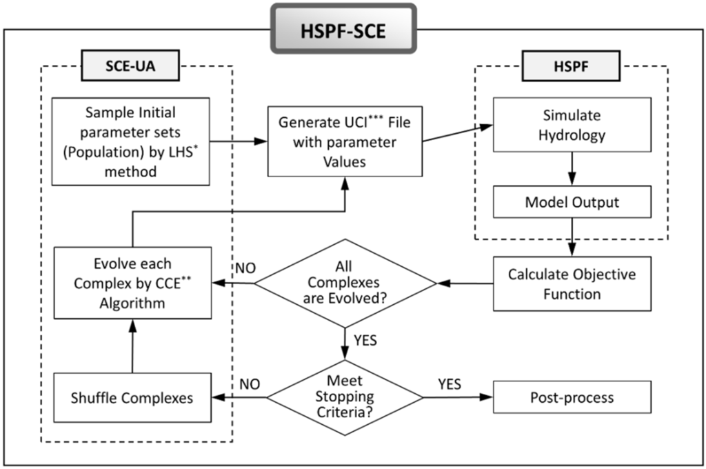
Figure 1. Flow chart for HSPF-SCE. Notes: LHS*: Latin Hypercube Sampling; CCE**: Competitive Complex Evolution; UCI***: User Control Interface.

Figure 1. Flow chart for HSPF-SCE. Notes: LHS*: Latin Hypercube Sampling; CCE**: Competitive Complex Evolution; UCI***: User Control Interface.

The HSPF-SCE application developed here allows a user to change the criteria to stop the SCE-UA optimization iterations. In the application presented here, HSPF-SCE stopped searching parameters when the difference between the average of the lowest ten objective function values and the lowest objective function value returned for any given population of parameter sets was ≤1.5%. It should be noted that a discussion about how one might choose the most appropriate convergence criterion or the number of complexes for the purpose of improving the efficiency of the optimization process goes beyond the scope of this study.

As mentioned earlier, HSPF-SCE provides a parallel computing option when multiple processors (or cores and threads) are available. In this study, a four-processor Intel(R) Core(TM) i7 CPU [email protected] chip was used allowing for parallel computing and parameter calibration. When using the HSPF-SCE tool, the parameter sampling and data flow happen in R. The HSPF code is not altered when implementing HSPF-SCE.

2.5. Objective Function

When calibrating hydrologic models, the calibration objective function(s) are typically goodness-of-fit measures (e.g., coefficient of determination (R²), Nash-Sutcliffe Efficiency (NSE)), with each assessing the degree of agreement between observed and simulated variables. Objective functions and the model performance criterion used to evaluate model calibration should be selected considering the objectives of any given modeling effort and the characteristics of the candidate objective function(s). Many previous studies have shown that using a single objective function may lead to unrealistic calibration results [5,7,8,47]. Using multiple objective functions, and thus multiple measures of goodness-of-fit, may allow one to consider different aspects of fit between simulated and observed variables [5]. As previously discussed, HSPEXP is a decision-support system that aids users who manually calibrate HSPF by offering expert advice about which parameters to adjust and how. HSPEXP guidance suggests the use of multiple objective criteria when assessing the adequacy of an HSPF hydrology calibration (Table 1).

Table 1. HSPEXP model performance criteria for hydrologic calibration of HSPF (revised from Kim et al. [5]).

Variable	Description	Criteria, % Error
Total volume	Error in total runoff volume for the calibration period	±10
Fifty-percent lowest flows	Error in the mean of the lowest 50 percent of the daily mean flows	±10
Ten-percent highest flows	Error in the mean of the highest 10 percent of the daily mean flows	±15
Storm peaks	Error in flow volumes for selected storms	±15
Seasonal volume error	Seasonal volume error, June-August runoff volume error minus December-February runoff volume error	±10
Summer storm volume error	Error in runoff volume for selected summer storms	±15

Table 1. HSPEXP model performance criteria for hydrologic calibration of HSPF (revised from Kim et al. [5]).

Variable	Description	Criteria, % Error
Total volume	Error in total runoff volume for the calibration period	±10
Fifty-percent lowest flows	Error in the mean of the lowest 50 percent of the daily mean flows	±10
Ten-percent highest flows	Error in the mean of the highest 10 percent of the daily mean flows	±15
Storm peaks	Error in flow volumes for selected storms	±15
Seasonal volume error	Seasonal volume error, June-August runoff volume error minus December-February runoff volume error	±10
Summer storm volume error	Error in runoff volume for selected summer storms	±15

Kim et al. [5], using PEST, applied a single composite objective function that combined six sub-objective functions based on the HSPEXP calibration criteria. In this study, we adopted an objective function uniformly weighted with six performance measures so that multiple evaluation aspects could be considered simultaneously in a single objective optimization framework (Table 2). For the objective function formulation used in this study, the objective function value can range from 0% to 600%, with 0% being perfect agreement between the simulated and observed data. It should be noted that the purpose of this study was to develop and demonstrate a reliable and efficient tool for automatic calibration tool/approach, not developing and evaluating the most appropriate calibration objective function.

Table 2. Objective functions used in the HSPF-SCE tool (revised from Kim et al. [5]).

Description	Formula
Objective function	$F\left(\theta \right)={\displaystyle {\displaystyle \sum }_{i=1}^6}{f}_i\left(\theta \right),\theta \in \Theta$
Absolute error of daily flow	$f_1\left(\theta \right)={\displaystyle {\displaystyle \sum }_{i=1}^N}\left|{\mathrm{Q}}_{\text{obs},\mathrm{i}}-{\mathrm{Q}}_{\text{sim},\mathrm{i}}\left(\mathrm{\theta }\right)\right|\bullet w_1$
Absolute error of 50% lowest flows exceedance	$f_2\left(\theta \right)=\left|E{X}_{obs,50\% lowest flow}-E{X}_{sim, 50\% lowest flow}(\theta )\right|\bullet w_2$
Absolute error of 10% highest flows exceedance	$f_3\left(\theta \right)=\left|E{X}_{obs,10\% highest flow}-E{X}_{sim, 10\% highest flow}(\theta )\right|\bullet w_3$
Absolute error of storm peak	$f_4\left(\theta \right)={\displaystyle {\displaystyle \sum }_{i=1}^{N_{st}}}\left|{\mathrm{P}}_{\text{obs},\mathrm{i}}-{\mathrm{P}}_{\text{sim},\mathrm{i}}\left(\mathrm{\theta }\right)\right|\bullet w_4$
Absolute error of seasonal volume	$f_5\left(\theta \right)={\displaystyle {\displaystyle \sum }_{j=1}^{N_{ss}}} \left(\left|{\displaystyle {\displaystyle \sum }_{i=1}^{n_j}}{\mathrm{Q}}_{\text{obs},\mathrm{i}}-{\displaystyle {\displaystyle \sum }_{i=1}^{n_j}}{\mathrm{Q}}_{\text{sim},\mathrm{i}}\left(\theta \right)\right|\bullet w_5\right)$
Absolute error of storm volume	$f_6\left(\theta \right)={\displaystyle {\displaystyle \sum }_{j=1}^{N_{st}}} \left(\left|{\displaystyle {\displaystyle \sum }_{i=1}^{m_j}}{\mathrm{Q}}_{\text{obs},\mathrm{i}}-{\displaystyle {\displaystyle \sum }_{i=1}^{m_j}}{\mathrm{Q}}_{\text{sim},\mathrm{i}}\left(\theta \right)\right|\bullet w_6\right)$

Table 2. Objective functions used in the HSPF-SCE tool (revised from Kim et al. [5]).

Description	Formula
Objective function	$F\left(\theta \right)={\displaystyle {\displaystyle \sum }_{i=1}^6}{f}_i\left(\theta \right),\theta \in \Theta$
Absolute error of daily flow	$f_1\left(\theta \right)={\displaystyle {\displaystyle \sum }_{i=1}^N}\left|{\mathrm{Q}}_{\text{obs},\mathrm{i}}-{\mathrm{Q}}_{\text{sim},\mathrm{i}}\left(\mathrm{\theta }\right)\right|\bullet w_1$
Absolute error of 50% lowest flows exceedance	$f_2\left(\theta \right)=\left|E{X}_{obs,50\% lowest flow}-E{X}_{sim, 50\% lowest flow}(\theta )\right|\bullet w_2$
Absolute error of 10% highest flows exceedance	$f_3\left(\theta \right)=\left|E{X}_{obs,10\% highest flow}-E{X}_{sim, 10\% highest flow}(\theta )\right|\bullet w_3$
Absolute error of storm peak	$f_4\left(\theta \right)={\displaystyle {\displaystyle \sum }_{i=1}^{N_{st}}}\left|{\mathrm{P}}_{\text{obs},\mathrm{i}}-{\mathrm{P}}_{\text{sim},\mathrm{i}}\left(\mathrm{\theta }\right)\right|\bullet w_4$
Absolute error of seasonal volume	$f_5\left(\theta \right)={\displaystyle {\displaystyle \sum }_{j=1}^{N_{ss}}} \left(\left|{\displaystyle {\displaystyle \sum }_{i=1}^{n_j}}{\mathrm{Q}}_{\text{obs},\mathrm{i}}-{\displaystyle {\displaystyle \sum }_{i=1}^{n_j}}{\mathrm{Q}}_{\text{sim},\mathrm{i}}\left(\theta \right)\right|\bullet w_5\right)$
Absolute error of storm volume	$f_6\left(\theta \right)={\displaystyle {\displaystyle \sum }_{j=1}^{N_{st}}} \left(\left|{\displaystyle {\displaystyle \sum }_{i=1}^{m_j}}{\mathrm{Q}}_{\text{obs},\mathrm{i}}-{\displaystyle {\displaystyle \sum }_{i=1}^{m_j}}{\mathrm{Q}}_{\text{sim},\mathrm{i}}\left(\theta \right)\right|\bullet w_6\right)$

In Table 2, $f_i\left(\theta \right)$ is the sub-objective function, θ is the parameter set, Θ is the feasible parameter range, Q is daily flow, EX is the fraction of time that stream flow equals or exceeds a specific flow rate, $N_{st}$ is the number of selected storm events, P is peak flow, $N_{ss}$ is the number of summer and winter months, $n_j$ is the number of time steps in each $j$ month, $m_j$ is the number of time steps in each $j$ storm event, and $w$ is a weighting factor.

2.6. Study Watersheds

Considering the availability of existing HSPF models that had been manually calibrated for bacteria TMDL development [48,49,50], three watersheds located in the Ridge and Valley Physiographic Province of Virginia were selected for this study (Figure 2). The Piney River watershed drains 123 km² in Amherst County and Nelson County, and its predominant land cover is forest (79%), followed by pasture (10%), cropland (6%), and residential (4%). A National Weather Service Cooperative Weather station is located at the Montebello Fish Hatchery (COOP ID: 445690) within the watershed, and daily streamflow discharge has been measured at the watershed outlet (gauging station ID: 02027500) by USGS. Model calibration and validation periods were set to 1 January 1991 to 31 December 1995 and 1 January 1996 to 31 December 2000, in which 21 and 16 storm events were identified, respectively.

Figure 2. Locations of the study watersheds.

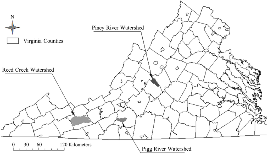
Figure 2. Locations of the study watersheds.

The Reed Creek watershed is 703.5 km² in size and located in Wythe County of Virginia. The watershed mainly consists of forest (52%) and pasture/hay land (38%) with residential (8%) and cropland (2%). A National Climatic Data Center’s (NCDC) Cooperative Weather station (Wytheville, COOP ID: 449301) is located 15 miles due west of the Reed Creek watershed outlet, where a USGS gauging station (ID: 03167000) is found. The hydrologic parameters of the HSPF model developed for the Reed Creek watershed were calibrated using streamflow measurements made between 1991 and 1998, and then the calibrated model was validated between 2001 and 2005. In the periods, 29 and 31 storm events were selected for the calibration and validation, respectively.

The Pigg River watershed, which is mainly located in Franklin County, Virginia, drains 186 km² directly into Roanoke River. The dominant land use in the watershed is forest at 72%, followed by pasture (23%), cropland (3%) and residential (2%). The watershed has a NCDC Cooperative Weather Station (Rocky Mount, COOP ID: 447338) and a USGS gauging station (ID: 02058400) at its outlet. The hydrologic simulation of HSPF was calibrated and validated using streamflow measurements made at the USGS station between 1 September 1989 and 31 December 1995 and between 1 June 1984 and 31 August 1989, in which 29 and 23 storm events were identified, respectively.

2.7. Selection of Calibration Parameters

HSPF represents hydrologic and hydraulic features of a watershed using fixed and process-related parameters [51]. Fixed parameters represent the hydraulic features of the drainage network and physical properties of the drainage basin, such as length, slope, width, depth and roughness of a watershed and areas covered by different soil types, land covers, and slopes. Process-related parameters are used to describe hillslope processes including rainfall interception, infiltration, runoff generation and routing, soil moisture storage, groundwater discharge into stream, and evapotranspiration [37,51].

Based on the HSPF model manual [45], sensitivity analysis [52], and the authors’ professional experience, nine parameters were selected for calibration (Table 3). The value for one of the nine parameters, UZSN, was allowed to vary between the winter season and non-winter season. Applying different values of UZSN for winter and non-winter periods increased the number of calibration parameters (N) to ten. The same value for each calibration parameter was used for all PERLNDs with the exception of INFILT. Since INFILT varied by PERLND, INFILT was changed by a multiplier which retains differences between INFILT values.

Table 3. Calibration parameters for hydrologic simulation of HSPF and their ranges [45].

Parameter	Definition	Typical Range	Possible Range
LZSN	Lower zone nominal storage, mm	76.2–203.2	50.8–381
UZSN *	Upper zone nominal storage, mm	2.54–25.4	1.27–50.8
INFILT	Index to infiltration capacity, mm/h	0.25–6.35	0.025–12.7
BASETP	Fraction of potential ET that can be sought from base flow	0–0.05	0–0.2
AGWETP	Fraction of remaining potential ET that can be satisfied from active groundwater storage	0–0.05	0–0.2
INTFW	Interflow inflow parameter	1.0–3.0	1.0–10.0
IRC	Interflow recession parameter, per day	0.5–0.7	0.3–0.85
AGWRC	Groundwater recession parameter, per day	0.92–0.99	0.85–0.999
DEEPFR	Fraction of groundwater inflow that goes to inactive groundwater	0–0.2	0–0.5

Note: * Value varied between winter season and non-winter season.

Table 3. Calibration parameters for hydrologic simulation of HSPF and their ranges [45].

Parameter	Definition	Typical Range	Possible Range
LZSN	Lower zone nominal storage, mm	76.2–203.2	50.8–381
UZSN *	Upper zone nominal storage, mm	2.54–25.4	1.27–50.8
INFILT	Index to infiltration capacity, mm/h	0.25–6.35	0.025–12.7
BASETP	Fraction of potential ET that can be sought from base flow	0–0.05	0–0.2
AGWETP	Fraction of remaining potential ET that can be satisfied from active groundwater storage	0–0.05	0–0.2
INTFW	Interflow inflow parameter	1.0–3.0	1.0–10.0
IRC	Interflow recession parameter, per day	0.5–0.7	0.3–0.85
AGWRC	Groundwater recession parameter, per day	0.92–0.99	0.85–0.999
DEEPFR	Fraction of groundwater inflow that goes to inactive groundwater	0–0.2	0–0.5

Note: * Value varied between winter season and non-winter season.

Possible ranges of parameter values found in the US EPA HSPF guidance document Technical Note 6 [45] were used to define the parameter space. For each of the three watershed models used here, the parameters not selected for calibration were fixed and left unchanged from the values that were used in the manually calibrated TMDL models.

2.8. Model Performance Evaluation

There is no firm consensus when it comes to acceptable hydrologic model performance measures; there is no one statistic that can be used to assess all aspects of model performance [38]. Thus, it is often recommended that one use multiple performance statistics in conjunction with graphical/visual assessments and other qualitative comparisons rather than relying on a single quantitative metric [38,53]. Having said that, most decision makers want definitive calibration targets or tolerance ranges [38]. Several studies have proposed general target ranges for various metrics to evaluate model performance. Donigian et al. [54] provided HSPF model users with general guidance on model evaluation statistics, and Duda et al. [38] noted that the tolerance range of percent error should be considered so that the modeler and model-results consumer may make a more informed assessment of the model’s performance. Moriasi et al. [53] suggested using performance statistics like NSE, percent bias (PBIAS) and RMSE-observations standard deviation ratio (RSR) and provided model evaluation guidelines for these measures (Table 4). A brief description of each Moriasi-suggested measure is provided below.

Table 4. General guidance for performance assessment of hydrologic modeling.

Statistics	Statistical Period	Very Good	Good	Satisfactory (Fair)	Unsatisfactory (Poor)	Ref.
R2 *	Daily	0.80 < R2 ≤ 1	0.70 < R2 ≤ 0.80	0.60 < R2 ≤ 0.70	R2 ≤ 0.60	[38]
R2	Monthly	0.86 < R2 ≤ 1	0.75 < R2 ≤ 0.86	0.65 < R2 ≤ 0.75	R2 ≤ 0.65	[38]
NSE	Monthly	0.75 < NSE ≤ 1.00	0.65 < NSE ≤ 0.75	0.50 < NSE ≤ 0.65	NSE ≤ 0.50	[53]
PBIAS	Monthly	PBIAS < ±10	±10 ≤ PBIAS < ±15	±15≤ PBIAS< ±25	PBIAS ≥ ±25	[53]
RSR	Monthly	0.00 ≤ RSR ≤ 0.50	0.50 < RSR ≤ 0.60	0.60< RSR ≤ 0.70	RSR > 0.70	[53]

Note: * Performance criteria ranges estimated from Figure 4 in Duda et al. [38].

Table 4. General guidance for performance assessment of hydrologic modeling.

Statistics	Statistical Period	Very Good	Good	Satisfactory (Fair)	Unsatisfactory (Poor)	Ref.
R2 *	Daily	0.80 < R2 ≤ 1	0.70 < R2 ≤ 0.80	0.60 < R2 ≤ 0.70	R2 ≤ 0.60	[38]
R2	Monthly	0.86 < R2 ≤ 1	0.75 < R2 ≤ 0.86	0.65 < R2 ≤ 0.75	R2 ≤ 0.65	[38]
NSE	Monthly	0.75 < NSE ≤ 1.00	0.65 < NSE ≤ 0.75	0.50 < NSE ≤ 0.65	NSE ≤ 0.50	[53]
PBIAS	Monthly	PBIAS < ±10	±10 ≤ PBIAS < ±15	±15≤ PBIAS< ±25	PBIAS ≥ ±25	[53]
RSR	Monthly	0.00 ≤ RSR ≤ 0.50	0.50 < RSR ≤ 0.60	0.60< RSR ≤ 0.70	RSR > 0.70	[53]

Note: * Performance criteria ranges estimated from Figure 4 in Duda et al. [38].

R² describes the degree of collinearity between simulated and measured flow (Nagelkerke, 1991), ranging from 0 to 1, and is given by

$$R^2=({\frac{{{\displaystyle \sum }}_{\mathrm{i}=1}^{\mathrm{N}}({\mathrm{Q}}_{\text{obs},\mathrm{i}}-{\overline{\mathrm{Q}}}_{\text{obs}})(({\mathrm{Q}}_{\text{sim},\mathrm{i}}-{\overline{\mathrm{Q}}}_{\text{sim}})}{{\left[{{\displaystyle \sum }}_{\mathrm{i}=1}^{\mathrm{N}}{({\mathrm{Q}}_{\text{obs},\mathrm{i}}-{\overline{\mathrm{Q}}}_{\text{obs}})}^2\right]}^{0.5}{\left[{{\displaystyle \sum }}_{\mathrm{i}=1}^{\mathrm{N}}{({\mathrm{Q}}_{\text{sim},\mathrm{i}}-{\overline{\mathrm{Q}}}_{\text{sim}})}^2\right]}^{0.5}})}^2$$

(1)

where N is the total number of flow data; ${\mathrm{Q}}_{obs}$ is observed flow; ${\mathrm{Q}}_{sim}$ is simulated flow; and the over bar denotes the mean for the entire evaluation time period. R² of 1 means a perfect linear relationship between two variables, while an R² of zero represents no linear relationship.

NSE is a normalized value that assesses the relative magnitude of the residual variance, ranging from minus infinity to 1 [55]. NSE values greater than zero imply that the model predictions are more accurate than the average of the observed data, and a NSE = 1 indicates the model predictions completely match observed data. NSE is one of the most widely used statistics for assessing agreement between two variables in hydrologic modeling [53], and its use was recommended by ASCE [56] and Legates and McCabe [57]. NSE is defined as

$$NSE=1-\frac{{{\displaystyle \sum }}_{\mathrm{i}=1}^{\mathrm{N}}{({\mathrm{Q}}_{\text{obs},\mathrm{i}}-{\mathrm{Q}}_{\text{sim},\mathrm{i}})}^2}{{{\displaystyle \sum }}_{\mathrm{i}=1}^{\mathrm{N}}{({\mathrm{Q}}_{\text{obs},\mathrm{i}}-{\overline{\mathrm{Q}}}_{\text{obs}})}^2}$$

(2)

PBIAS represents the overall agreement between two variables [58]. A PBIAS of zero means there is no overall bias in the simulated output of interest compared to the observed data. Positive and negative PBIAS values indicate over-estimation and under-estimation bias of the model, respectively [58]. PBIAS expressed as a percentage is given by

$$PBIAS=\frac{{{\displaystyle \sum }}_{\mathrm{i}=1}^{\mathrm{N}}({\mathrm{Q}}_{\text{sim},\mathrm{i}}-{\mathrm{Q}}_{\text{obs},\mathrm{i}})\times 100}{{{\displaystyle \sum }}_{\mathrm{i}=1}^{\mathrm{N}}({\mathrm{Q}}_{\text{obs},\mathrm{i}})}$$

(3)

Root mean square error (RMSE) is an absolute error measure commonly used in hydrologic modeling. Chu and Shirmohammadi [59] and Singh et al. [60] introduced RSR to facilitate relative comparison between RMSE values calculated for estimations in different units and scales by normalizing RMSE with the standard deviation of the observed data. RSR can vary from 0 to a large positive value, and a lower RSR value indicates better model performance [53]. RSR is defined as

$$RSR=\frac{\text{RMSE}}{{\text{STDEV}}_{\text{obs}}}=\frac{\sqrt{{{\displaystyle \sum }}_{\mathrm{i}=1}^{\mathrm{N}}{({\mathrm{Q}}_{\text{obs},\mathrm{i}}-{\mathrm{Q}}_{\text{sim},\mathrm{i}})}^2}}{\sqrt{{{\displaystyle \sum }}_{\mathrm{i}=1}^{\mathrm{N}}{({\mathrm{Q}}_{\text{obs},\mathrm{i}}-{\overline{\mathrm{Q}}}_{\text{obs}})}^2}}$$

(4)

In this study, calibrated HSPF hydrologic simulations were evaluated with statistical measures of R², NSE, PBIAS, and RSR as wells as visual comparison of observed and simulated flow time series and flow duration curves.

3. Results and Discussion

3.1. Assessing Acceptable Estimated Parameter Sets

In this study, three HSPF hydrologic models were calibrated using the HSPF-SCE auto calibration tool. The HSPF-SCE tool was allowed to calibrate nine parameters, with one of those allowed to vary seasonally for a total of ten calibration parameters. In the calibration processes, the SCE-UA algorithm identified multiple parameter sets that satisfied the six HSPEXP model performance criteria while minimizing objective function values. For example, for the Reed Creek watershed, 252 parameter sets out of 504 possible parameter sets were found to meet all the six HSPXEP criteria. Figure 3 shows the Reed Creek distribution of the objective function values on the left y-axis and the number of HSPEXP criteria satisfied by the parameter sets in the last iteration of the optimization process on the right y-axis. Parameter sets began meeting all six HSPEXP criteria once the value of the objective function decreased to approximately 50%. The minimum objective function value was 11.6%. For the Piney River and Pigg River watersheds, 159 and 141 parameter sets satisfied all six HSPEXP criteria, respectively. The parameter sets that met all six HSPEXP calibration criteria are referred to herein as “qualified” parameter sets.

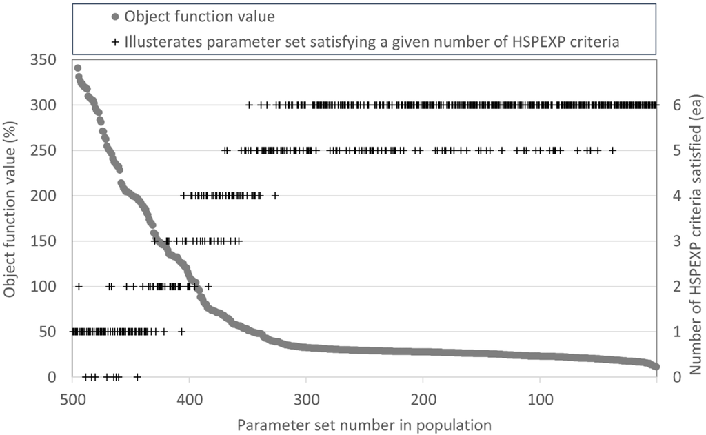
Figure 3. Objective function values and the number of HSPEXP criteria met by the final parameter set population using the SCE-UA algorithm of HSPF-SCE (Reed Creek watershed).

Figure 3. Objective function values and the number of HSPEXP criteria met by the final parameter set population using the SCE-UA algorithm of HSPF-SCE (Reed Creek watershed).

Performance statistics produced by the qualified parameter sets are shown in Figure 4. For the Reed Creek watershed, hydrologic simulation using the 252 qualified parameter sets produced statistics in the “very good” ranges for monthly PBIAS, monthly NSE, and monthly RSR with some “good” measures for monthly R² (Table 4). The 159 qualified parameter sets for the Piney River watershed were in the ranges of between “good” and “fair” for monthly NSE and monthly RSR, “very good” for monthly PBIAS, but monthly R² values were in between “fair” and “poor”. On the other hand, the 141 qualified parameter for the Pigg River watershed yielded relatively unsatisfactory performance statistics, and values of monthly NSE, monthly RSR, monthly R² and daily R² were classified as “poor”. Karst topography including sink holes and springs that frequently appear in the Ridge and Valley physiographic region of Virginia [61] could be one possible reason for the poor model performance in the Pigg River watershed. HSPF has limited groundwater simulation capabilities, and representing karst hydrology using HSPF is challenging.

Once multiple parameter sets that met all the HSPEXP criteria were identified, a single parameter set expected to best represent the hydrologic processes of a study watershed was selected from the pool of qualified parameter sets. This selection was based on model performance statistics, visual comparisons of various model output graphics (e.g., Figure 5), and best professional judgment. For example, for the Reed Creek watershed, 160 parameter sets out of 252 were qualified, meaning they satisfied all six HSPEXP criteria for both the calibration and validation period. The 160 qualified parameter sets were then classified into groups based on five performance statistics as shown in Table 5 and Table 6. Parameter sets belonging to the same group were regarded as equal in terms of model performance. In addition to the comparison of performance statistics presented in Table 5 and Table 6, the qualified parameter sets classified into Group 1 were further assessed by visually comparing hydrographs and flow duration curve plots simulated using those Group 1 parameter sets.

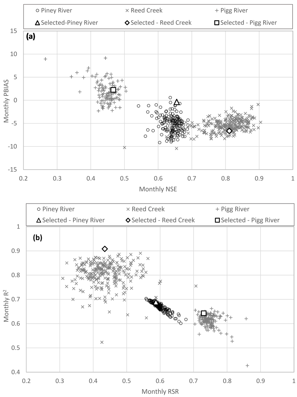
Figure 4. Qualified parameter set model performance plots. Data generated by running HSPF with each qualified parameter set, then comparing observed and simulated model output using four model performance measures (a) Monthly PBIAS and Monthly NSE; and (b) Monthly R² and Monthly RSR. The square, triangle, and diamond correspond to the parameter set selected by the authors for subsequent HSPF simulations and model performance evaluation.

Figure 4. Qualified parameter set model performance plots. Data generated by running HSPF with each qualified parameter set, then comparing observed and simulated model output using four model performance measures (a) Monthly PBIAS and Monthly NSE; and (b) Monthly R² and Monthly RSR. The square, triangle, and diamond correspond to the parameter set selected by the authors for subsequent HSPF simulations and model performance evaluation.

Figure 5. Comparison of the observed and simulated daily hydrographs with parameter set No. 40 (a,c) and No. 179 (b,d) for the Reed Creek watershed; (a,b) are daily log-scale hydrographs; and (c,d) are flow duration curves of daily flow.

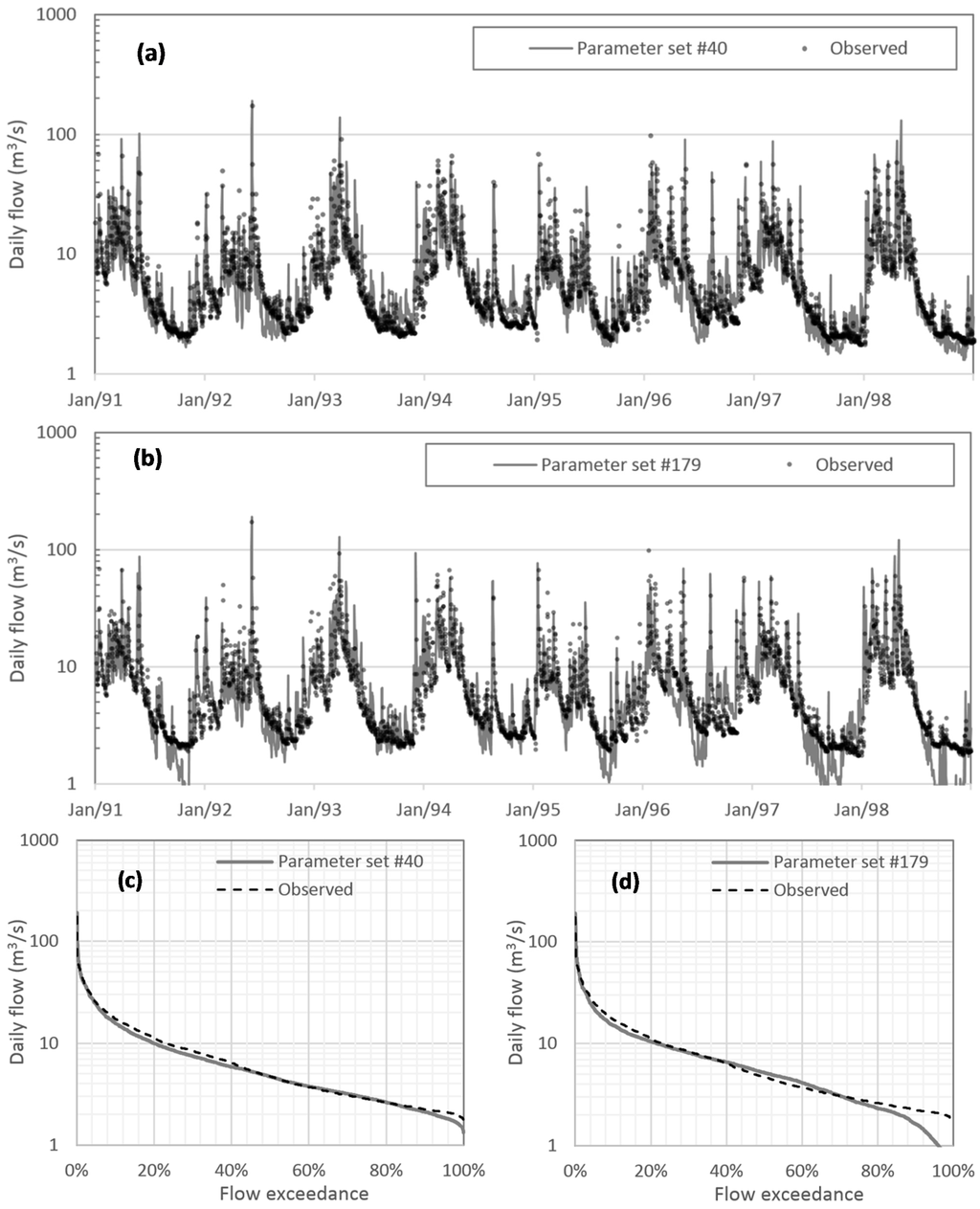
Figure 5. Comparison of the observed and simulated daily hydrographs with parameter set No. 40 (a,c) and No. 179 (b,d) for the Reed Creek watershed; (a,b) are daily log-scale hydrographs; and (c,d) are flow duration curves of daily flow.

Table 5. Classification of the parameter sets identified by HSPF-SCE in terms of model performance statistics (for the Reed Creek watershed).

Group	Parameter Set ID	Daily R2		Monthly R2		Monthly RSR		Monthly PBIAS		Monthly NSE
Group 1	35	0.608	Fair	0.873	Very good	0.408	Very good	−4.130	Very good	0.834	Very good
	40 *	0.632		0.908		0.435		−6.626		0.811
	95	0.605		0.866		0.401		−4.857		0.839
	98	0.601		0.862		0.444		−6.180		0.803
	142	0.606		0.870		0.361		−3.277		0.870
	171	0.626		0.886		0.477		−4.539		0.772
	179	0.610		0.864		0.345		−3.826		0.881
	196	0.615		0.872		0.414		−5.071		0.828
	256	0.611		0.869		0.432		−4.841		0.814
	278	0.609		0.866		0.386		−4.393		0.851
Group 2	192	0.622	Fair	0.885	Very good	0.512	Good	−6.954	Very good	0.737	Good
	221	0.603		0.871		0.534		−7.817		0.715
	242	0.605		0.872		0.502		−3.543		0.748
Group 3	157	0.601	Fair	0.841	Good	0.549	Good	−5.498	Very good	0.699	Good
Group 4	216	0.593	Poor	0.868	Very good	0.484	Very good	−7.103	Very good	0.765	Very good
	204	0.592		0.879		0.474		−4.970		0.776
	212	0.598		0.870		0.450		−5.845		0.798

Note: * A parameter set selected as the most representative at the final selection.

Table 5. Classification of the parameter sets identified by HSPF-SCE in terms of model performance statistics (for the Reed Creek watershed).

Group	Parameter Set ID	Daily R2		Monthly R2		Monthly RSR		Monthly PBIAS		Monthly NSE
Group 1	35	0.608	Fair	0.873	Very good	0.408	Very good	−4.130	Very good	0.834	Very good
	40 *	0.632		0.908		0.435		−6.626		0.811
	95	0.605		0.866		0.401		−4.857		0.839
	98	0.601		0.862		0.444		−6.180		0.803
	142	0.606		0.870		0.361		−3.277		0.870
	171	0.626		0.886		0.477		−4.539		0.772
	179	0.610		0.864		0.345		−3.826		0.881
	196	0.615		0.872		0.414		−5.071		0.828
	256	0.611		0.869		0.432		−4.841		0.814
	278	0.609		0.866		0.386		−4.393		0.851
Group 2	192	0.622	Fair	0.885	Very good	0.512	Good	−6.954	Very good	0.737	Good
	221	0.603		0.871		0.534		−7.817		0.715
	242	0.605		0.872		0.502		−3.543		0.748
Group 3	157	0.601	Fair	0.841	Good	0.549	Good	−5.498	Very good	0.699	Good
Group 4	216	0.593	Poor	0.868	Very good	0.484	Very good	−7.103	Very good	0.765	Very good
	204	0.592		0.879		0.474		−4.970		0.776
	212	0.598		0.870		0.450		−5.845		0.798

Note: * A parameter set selected as the most representative at the final selection.

Table 6. The HSPEXP criteria values of Groups 1 to 4 (for the Reed Creek watershed).

Group	Parameter set ID	Total Volume (±10%)	50% Lowest Flows (±10%)	10% Highest Flows (±15%)	Storm Peaks (±15%)	Seasonal Volume (±10%)	Seasonal Storm Volume (±15%)
Group 1	35	−4.77	−6.15	−2.83	2.13	1.44	−1.60
	40 *	−4.68	−0.52	−0.70	6.60	6.66	−0.26
	95	−3.97	−7.24	−1.41	5.90	3.49	−1.26
	98	−5.40	−3.49	−4.64	0.84	5.68	−3.23
	142	−6.32	−5.45	−2.91	5.17	3.64	−2.44
	171	−4.07	−9.80	−1.90	2.47	8.08	−0.72
	179	−4.99	−5.09	−5.80	1.49	5.30	−4.55
	196	−4.38	−5.77	−2.76	3.63	9.44	−2.02
	256	−6.61	−9.81	−5.09	3.23	0.85	−4.23
	278	−5.62	−9.65	−3.33	3.47	6.48	−2.73
Group 2	192	−3.93	−6.52	−4.83	3.75	4.17	−4.69
	221	−4.94	−1.88	−2.69	6.03	9.71	−3.30
	242	−5.65	−2.48	−4.89	4.17	7.47	−4.67
Group 3	157	−2.27	−8.62	1.46	7.00	−3.53	3.50
Group 4	216	−5.53	1.83	0.66	9.43	9.78	−1.21
	204	−3.92	−2.08	2.83	8.84	8.61	1.87
	212	−5.63	−8.08	0.53	9.59	4.45	−0.12

Note: * A parameter set selected as the most representative at the final selection.

Table 6. The HSPEXP criteria values of Groups 1 to 4 (for the Reed Creek watershed).

Group	Parameter set ID	Total Volume (±10%)	50% Lowest Flows (±10%)	10% Highest Flows (±15%)	Storm Peaks (±15%)	Seasonal Volume (±10%)	Seasonal Storm Volume (±15%)
Group 1	35	−4.77	−6.15	−2.83	2.13	1.44	−1.60
	40 *	−4.68	−0.52	−0.70	6.60	6.66	−0.26
	95	−3.97	−7.24	−1.41	5.90	3.49	−1.26
	98	−5.40	−3.49	−4.64	0.84	5.68	−3.23
	142	−6.32	−5.45	−2.91	5.17	3.64	−2.44
	171	−4.07	−9.80	−1.90	2.47	8.08	−0.72
	179	−4.99	−5.09	−5.80	1.49	5.30	−4.55
	196	−4.38	−5.77	−2.76	3.63	9.44	−2.02
	256	−6.61	−9.81	−5.09	3.23	0.85	−4.23
	278	−5.62	−9.65	−3.33	3.47	6.48	−2.73
Group 2	192	−3.93	−6.52	−4.83	3.75	4.17	−4.69
	221	−4.94	−1.88	−2.69	6.03	9.71	−3.30
	242	−5.65	−2.48	−4.89	4.17	7.47	−4.67
Group 3	157	−2.27	−8.62	1.46	7.00	−3.53	3.50
Group 4	216	−5.53	1.83	0.66	9.43	9.78	−1.21
	204	−3.92	−2.08	2.83	8.84	8.61	1.87
	212	−5.63	−8.08	0.53	9.59	4.45	−0.12

Note: * A parameter set selected as the most representative at the final selection.

To illustrate the graphical/visual model performance evaluation, the daily flow time-series and flow duration curve simulated using two of the qualified parameter sets (i.e., No. 40 and No. 179 in Table 5 and Table 6) are plotted in Figure 5. Although parameter set No. 179 provided better monthly RSR, PBIAS, and NSE than did No. 40 (Table 5), the graphical comparison (Figure 5) clearly shows parameter set No. 40 yielded a better match to the observed flow. Thus, parameter set No. 40 was selected as the final parameter set to simulate the hydrology for the Reed Creek watershed. The same parameter selection process was applied to the Pigg and Piney River watersheds.

3.2. Comparing Automated and Manual Calibration Parameter Sets

Manually calibrated parameter values were compared with the selected qualified parameter set identified by HSPF-SCE. Table 7 presents the comparison for all three watersheds, while Figure 6 illustrates those comparisons graphically for the Reed Creek watershed. The manual and automated approaches provided quite different ranges for some parameters: LZSN, UZSN, INFILT, BASETP, and AGWETP. Figure 6 shows box plots for the automated calibrated parameters for the Reed Creek model qualified parameter sets. In Figure 6, the interquartile ranges (IQR) of selected parameters (INFILT, AGWRC, DEEPFR, BASETP, AGWETP, IRC, INTFW, and UZSN–winter season) do not include the manually calibrated values implying that manual calibration is likely to fall in a local optimum in the parameter space. This finding does not agree with Kim et al. [5], who found general agreement among manually calibrated and PEST calibrated parameter values. The discrepancy between this study and Kim et al. [5] might be due to the use of different automated optimization algorithms (SCE-UA vs. PEST) and subjectivity in selecting a final parameter set from the pool of qualified parameter sets.

Table 7. Comparison of parameter values calibrated by HSPF-SCE and manually.

Parameter	Piney River Watershed		Pigg River Watershed		Reed Creek Watershed
	HSPF-SCE	Manual	HSPF-SCE	Manual	HSPF-SCE	Manual
LZSN	170.993	165.100	261.493	228.600	58.115	177.800
UZSN	31.496 *, 26.416 **	24.130–34.290	20.828 *, 27.940 **	8.890–25.400	31.750 *, 29.210 **	5.080 *, 25.400 **
INFILT	0.432–3.810	0.229–1.981	1.524–3.912	2.438–6.223	0.711–4.902	0.508–3.505
BASETP	0.072	0.000	0.091	0.150	0.106	0.050–0.060
AGWETP	0.007	0.000	0.022	0.100	0.058	0.010
INTFW	1.999	3.000	1.621	1.000	2.305	2.000
IRC	0.598	0.810	0.544	0.300	0.698	0.700
AGWRC	0.959	0.960, 0.965	0.994	0.990	0.992	0.990
DEEPFR	0.008	0.010	0.165	0.100	0.033	0.050

Notes: * For Winter (December through February); ** For Spring to Fall (March through November).

Table 7. Comparison of parameter values calibrated by HSPF-SCE and manually.

Parameter	Piney River Watershed		Pigg River Watershed		Reed Creek Watershed
	HSPF-SCE	Manual	HSPF-SCE	Manual	HSPF-SCE	Manual
LZSN	170.993	165.100	261.493	228.600	58.115	177.800
UZSN	31.496 *, 26.416 **	24.130–34.290	20.828 *, 27.940 **	8.890–25.400	31.750 *, 29.210 **	5.080 *, 25.400 **
INFILT	0.432–3.810	0.229–1.981	1.524–3.912	2.438–6.223	0.711–4.902	0.508–3.505
BASETP	0.072	0.000	0.091	0.150	0.106	0.050–0.060
AGWETP	0.007	0.000	0.022	0.100	0.058	0.010
INTFW	1.999	3.000	1.621	1.000	2.305	2.000
IRC	0.598	0.810	0.544	0.300	0.698	0.700
AGWRC	0.959	0.960, 0.965	0.994	0.990	0.992	0.990
DEEPFR	0.008	0.010	0.165	0.100	0.033	0.050

Notes: * For Winter (December through February); ** For Spring to Fall (March through November).

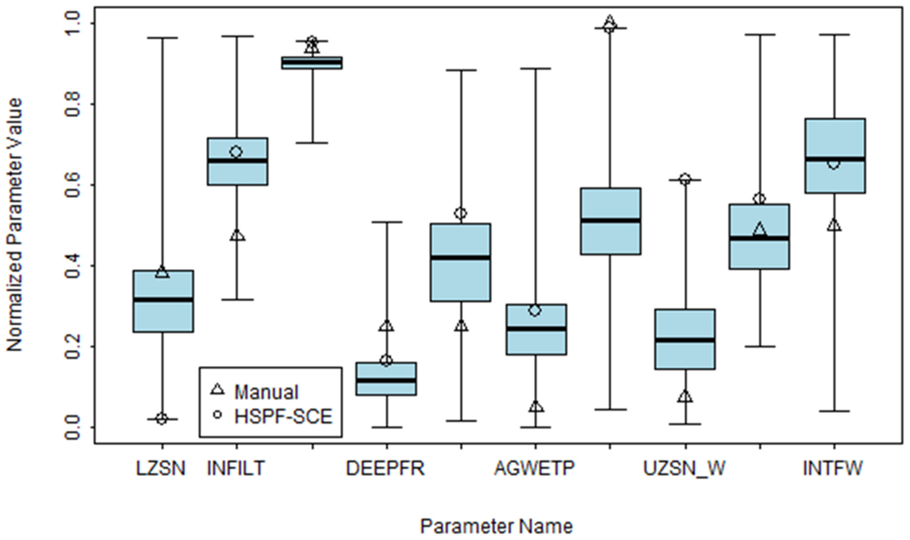
Figure 6. Comparison of parameter values calibrated by the HSPF-SCE and manually calibrated parameter values for the Reed Creek watershed (UZSN_W is for winter season and UZSN_N is for non-winter season).

Figure 6. Comparison of parameter values calibrated by the HSPF-SCE and manually calibrated parameter values for the Reed Creek watershed (UZSN_W is for winter season and UZSN_N is for non-winter season).

3.3. Comparison of Model Performance between Automatic and Manual Calibration

Hydrographs simulated with the selected qualified parameter sets were evaluated in terms of the six HSPEXP criteria. As seen in Table 8, both manually and HSPF-SCE calibrated parameters produced model output that meet all the criteria. The HSPF-SCE calibrated parameter set consistently provided lower bias in simulation of total volume compared to the manually calibrated parameters. Goodness-of-fit measures for the selected parameter sets are presented in Table 9. In general, the selected parameter values calibrated using HSPF-SCE provided performance statistics better than or equivalent to those calibrated manually. The measures of the Piney River watershed indicated “fair” to “very good” in the calibration period and “good” to “very good” in the validation period for both calibration methods. For the Reed Creek watershed, relatively great differences were found in the performance statistics compared to the other watersheds. HSPF-SCE provided statistics in the “very good” range, while those of the manual method were in “fair” to “good” in the both the calibration and validation periods. The selected parameter set for the Pigg River watershed gave “unsatisfactory” modeling results in terms of R², RSR and NSE in the calibration period. In all the cases, PBIAS values fell in the “very good” range.

Piney River observed and simulated daily and monthly flow and flow exceedance curves are compared in Figure 7, Figure 8 and Figure 9. Overall, flows simulated using the HSPF-SCE calibrated parameters are similar to those simulated using the manual calibration method, especially for baseflow and high peaks (Figure 7). In the Pigg River watershed, overestimation and underestimation of stream flow are found in 1992 of the calibration period and the first year of the validation period, respectively. The HSPF-SCE calibrated parameter values resulted in better simulation results under the low-flow conditions of 1986 and 1991 than the manually calibrated parameters. In general, the HSPF-SCE calibrated parameters provided better agreement with the observed flow than did the manually calibrated parameters (Figure 8). In the Reed Creek watershed, the simulated and observed flow hydrographs showed better agreement in the calibration period than the validation period (Figure 9). The relative difference of the model performance for the calibration and validation periods is reflected in the statistics presented in Table 9.

Table 8. Comparison of model performance achieved by the calibrated parameters in terms of the six HSPEXP criteria.

Watershed	Calibration Method	Periods	Total Volume (±10%)	50% Lowest Flows (±10%)	10% Highest Flows (±15%)	Storm Peaks (±15%)	Seasonal Volume (±10%)	Seasonal Storm Volume (±15%)
Piney River	HSPF-SCE	Calibration	−0.3	6.9	4.0	2.6	1.1	13.2
		Validation	−8.5	−0.5	−6.2	−7.0	−8.6	14. 8
	Manual	Calibration	0.7	5.9	5.9	6.5	−0.5	10.5
		Validation	−7.8	−0.5	−5.3	−5.8	−9.2	12.2
Pigg River	HSPF-SCE	Calibration	2.4	−4.3	9.0	−2.7	3.7	14.6
		Validation	0.9	−7.3	3.9	−13.5	9.0	2.6
	Manual	Calibration	7.8	−3.3	13.2	−0.3	1.5	14.4
		Validation	7.1	2.6	2.4	−10.4	2.8	−2.0
Reed Creek	HSPF-SCE	Calibration	−4.7	−0.5	−0.7	6.6	6.7	13.7
		Validation	−6.8	1.1	−1.8	−14.3	−1.0	−6.4
	Manual	Calibration	−5.9	8.2	−4.0	6.5	5.0	12.4
		Validation	−6.8	3.9	−3.5	−6.9	6.9	−6.8

Table 8. Comparison of model performance achieved by the calibrated parameters in terms of the six HSPEXP criteria.

Watershed	Calibration Method	Periods	Total Volume (±10%)	50% Lowest Flows (±10%)	10% Highest Flows (±15%)	Storm Peaks (±15%)	Seasonal Volume (±10%)	Seasonal Storm Volume (±15%)
Piney River	HSPF-SCE	Calibration	−0.3	6.9	4.0	2.6	1.1	13.2
		Validation	−8.5	−0.5	−6.2	−7.0	−8.6	14. 8
	Manual	Calibration	0.7	5.9	5.9	6.5	−0.5	10.5
		Validation	−7.8	−0.5	−5.3	−5.8	−9.2	12.2
Pigg River	HSPF-SCE	Calibration	2.4	−4.3	9.0	−2.7	3.7	14.6
		Validation	0.9	−7.3	3.9	−13.5	9.0	2.6
	Manual	Calibration	7.8	−3.3	13.2	−0.3	1.5	14.4
		Validation	7.1	2.6	2.4	−10.4	2.8	−2.0
Reed Creek	HSPF-SCE	Calibration	−4.7	−0.5	−0.7	6.6	6.7	13.7
		Validation	−6.8	1.1	−1.8	−14.3	−1.0	−6.4
	Manual	Calibration	−5.9	8.2	−4.0	6.5	5.0	12.4
		Validation	−6.8	3.9	−3.5	−6.9	6.9	−6.8

Table 9. Comparison of the model performance achieved by the calibrated parameters in terms of common goodness-of-fit measures.

Watershed	Calibration Method	Temporal Scale	Calibration				Validation
			R2	RSR	PBIAS	NSE	R2	RSR	PBIAS	NSE
Piney River	HSPF-SCE	Daily	0.66	0.97	−0.29	0.05	0.79	0.47	−8.52	0.78
		Monthly	0.69	0.59	−0.37	0.66	0.82	0.44	−8.50	0.81
	Manual	Daily	0.29	1.02	0.58	−0.03	0.79	0.48	−7.81	0.77
		Monthly	0.68	0.60	0.40	0.63	0.82	0.45	−7.79	0.80
Pigg River	HSPF-SCE	Daily	0.35	0.88	2.37	0.22	0.55	0.67	0.94	0.55
		Monthly	0.64	0.73	2.26	0.47	0.84	0.42	0.76	0.83
	Manual	Daily	0.37	0.90	8.01	0.19	0.57	0.66	7.22	0.57
		Monthly	0.65	0.80	8.00	0.36	0.85	0.41	7.07	0.83
Reed Creek	HSPF-SCE	Daily	0.63	0.67	−4.68	0.56	0.65	0.61	−6.79	0.63
		Monthly	0.91	0.43	−6.63	0.81	0.78	0.48	−6.86	0.77
	Manual	Daily	0.51	0.79	−5.89	0.37	0.57	0.67	−6.79	0.55
		Monthly	0.70	0.56	−6.27	0.69	0.59	0.65	−7.03	0.57

Table 9. Comparison of the model performance achieved by the calibrated parameters in terms of common goodness-of-fit measures.

Watershed	Calibration Method	Temporal Scale	Calibration				Validation
			R2	RSR	PBIAS	NSE	R2	RSR	PBIAS	NSE
Piney River	HSPF-SCE	Daily	0.66	0.97	−0.29	0.05	0.79	0.47	−8.52	0.78
		Monthly	0.69	0.59	−0.37	0.66	0.82	0.44	−8.50	0.81
	Manual	Daily	0.29	1.02	0.58	−0.03	0.79	0.48	−7.81	0.77
		Monthly	0.68	0.60	0.40	0.63	0.82	0.45	−7.79	0.80
Pigg River	HSPF-SCE	Daily	0.35	0.88	2.37	0.22	0.55	0.67	0.94	0.55
		Monthly	0.64	0.73	2.26	0.47	0.84	0.42	0.76	0.83
	Manual	Daily	0.37	0.90	8.01	0.19	0.57	0.66	7.22	0.57
		Monthly	0.65	0.80	8.00	0.36	0.85	0.41	7.07	0.83
Reed Creek	HSPF-SCE	Daily	0.63	0.67	−4.68	0.56	0.65	0.61	−6.79	0.63
		Monthly	0.91	0.43	−6.63	0.81	0.78	0.48	−6.86	0.77
	Manual	Daily	0.51	0.79	−5.89	0.37	0.57	0.67	−6.79	0.55
		Monthly	0.70	0.56	−6.27	0.69	0.59	0.65	−7.03	0.57

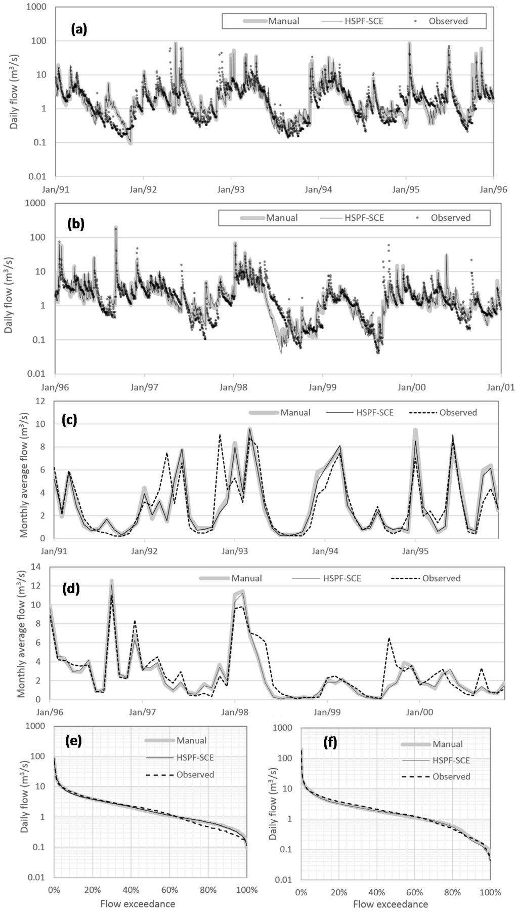
Figure 7. Comparison of the observed and simulated daily and monthly hydrographs with the selected parameter set for the Piney River watershed. (a,b) daily hydrographs; (c,d) monthly hydrographs; and (e,f) flow duration curves of daily flow.

Figure 7. Comparison of the observed and simulated daily and monthly hydrographs with the selected parameter set for the Piney River watershed. (a,b) daily hydrographs; (c,d) monthly hydrographs; and (e,f) flow duration curves of daily flow.

Figure 8. Comparison of the observed and simulated daily and monthly hydrographs with the selected parameter set for the Pigg River watershed. (a,b) daily hydrographs; (c,d) monthly hydrographs; and (e,f) flow duration curves of daily flow.

Figure 8. Comparison of the observed and simulated daily and monthly hydrographs with the selected parameter set for the Pigg River watershed. (a,b) daily hydrographs; (c,d) monthly hydrographs; and (e,f) flow duration curves of daily flow.

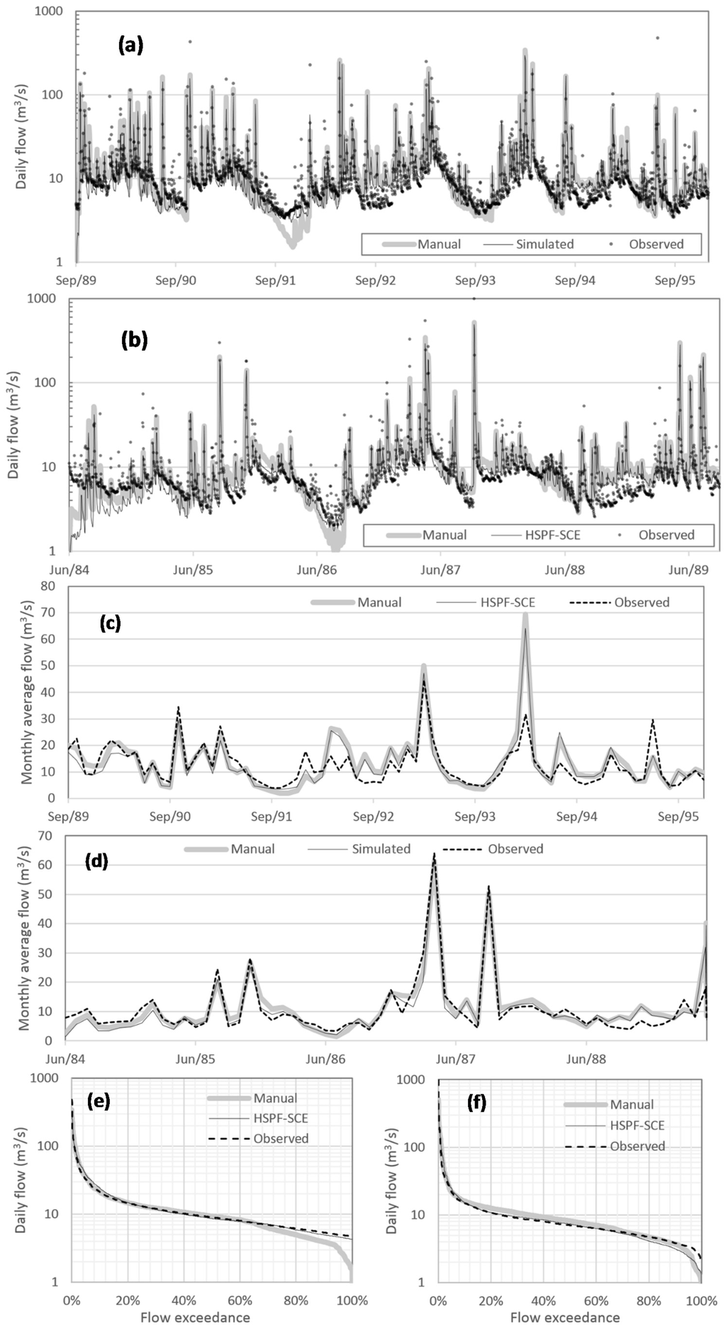
Figure 9. Comparison of the observed and simulated daily and monthly hydrographs with the selected parameter set for the Reed Creek watershed. (a,b) daily hydrographs; (c,d) monthly hydrographs; and (e,f) flow duration curves of daily flow.

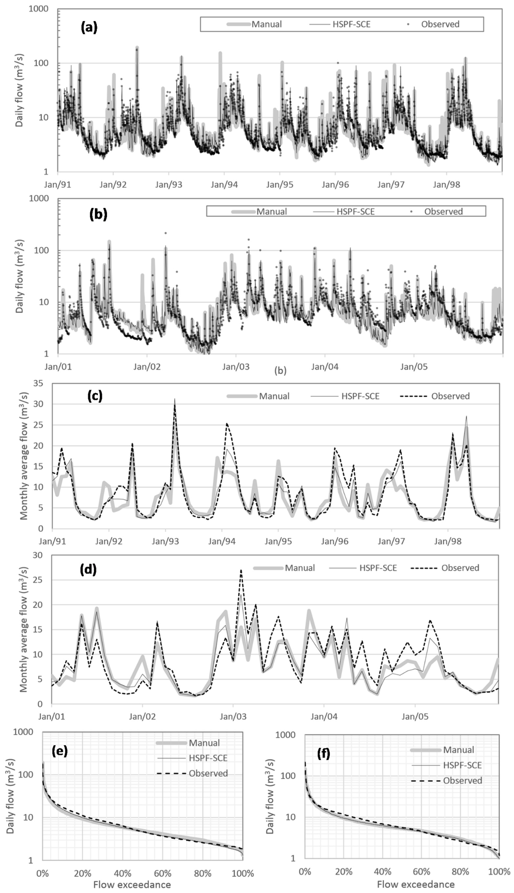
Figure 9. Comparison of the observed and simulated daily and monthly hydrographs with the selected parameter set for the Reed Creek watershed. (a,b) daily hydrographs; (c,d) monthly hydrographs; and (e,f) flow duration curves of daily flow.

The time required to perform the calibration for the study watersheds was compared between the automated and manual calibration methods (Table 10). The computational time required by HSPF-SCE employing between one and four processors was documented for the Pigg River watershed. Parallel computing using two and four processors was 47% and 66% faster than using a single processor, respectively, which indicates that parallel processing is indeed more efficient. Comparing the time required for the automated and manual calibration, for the Pigg River watershed, manual calibration took 3.8 times as many hours when compared to the parallel processing time requirement. For the Piney and Reed Creek watersheds, manual calibration required 4.3 and 1.5 times longer than the automated calibration, respectively. The numbers of model runs required by HSPF-SCE and the manual method were relatively small for the Pigg River watershed and larger for the Reed Creek watershed, implying that parameter calibration was more difficult for the Reed Creek watershed than the Pigg River watershed. The manual calibration time spent was estimated based on data collected during the respective TMDL development projects. All calibrations were performed on an Intel 2.93 GHz quad core machine with 4 GB of RAM on Windows 8 in a 64-bit environment. The simulation time estimates shown in Table 10 for the HSPF-SCE account for computational time only. As presented here, there is an additional step that must be completed after HSPF-SCE has identified the pool of qualified parameter sets; this is the graphical comparison that must be performed by the modeler to select the final parameter set from the qualified parameter sets. The authors estimate that for each of the study watersheds presented here, this process of selecting the final parameter set from the qualified parameter sets took about one day (8 h).

Table 10. Comparison of calibration time spent between automated and manual method.

Calibration Method	Watershed	Number of Processor	Total Simulation Time (h)	Total Number of Model Runs	Time Required to Complete Calibration (h)
HSPF-SCE	Pigg River	1	25.12	19,656	33.12
		2	13.21	19,656	21.21
		4	8.51	19,656	16.51
	Piney River	4	16.88	20,664	24.88
	Reed Creek	4	62.37	38,304	70.37
Manual	Pigg River	1	62.72	135	62.72
	Piney River		107.07	280	107.07
	Reed Creek		106.40	310	106.40

Table 10. Comparison of calibration time spent between automated and manual method.

Calibration Method	Watershed	Number of Processor	Total Simulation Time (h)	Total Number of Model Runs	Time Required to Complete Calibration (h)
HSPF-SCE	Pigg River	1	25.12	19,656	33.12
		2	13.21	19,656	21.21
		4	8.51	19,656	16.51
	Piney River	4	16.88	20,664	24.88
	Reed Creek	4	62.37	38,304	70.37
Manual	Pigg River	1	62.72	135	62.72
	Piney River		107.07	280	107.07
	Reed Creek		106.40	310	106.40

4. Summary and Conclusions

An automated calibration tool for HSPF was developed, HSPF-SCE, and its capability/applicability was examined with existing HSPF models developed for three Virginia watersheds. Utilizing the R software environment, the new tool links the HSPF model to the SCE-UA optimization algorithm without any modification of the HSPF model. The R software environment also allows HSPF-SCE to utilize parallel computing resources, making the tool computationally efficient. HSPF models that had been previously assembled for bacteria TMDL development purposes in three watersheds in Virginia were calibrated using HSPF-SCE. Model performance for the auto-calibrated and manually-calibrated models was compared.

HSPF-SCE calibrated parameters outperformed the manually calibrated parameters in terms of model performance statistics and in terms of how long it took to calibrate the model (HSPF-SCE was quicker). HSPF-SCE identified multiple qualified hydrologic parameter sets satisfying all six HSPEXP criteria, suggesting HSPF-SCE can be an effective tool for hydrologic calibration of HSPF. Manually calibrated parameter values often fell outside of the IQRs developed using the qualified parameter set values, indicating the manual calibration method may fall in a local optimum in the parameter calibration space. It was also demonstrated that satisfying the HSPEXP criteria does not necessarily imply good model performance in terms of commonly used statistics such as NSE, R², RSR, and PBIAS.

The applicability of the HSPF-SCE tool to efficiently and effectively calibrate the HSPF model was successfully demonstrated in this study. However, potential improvements remain. It is worth mentioning that since the tool itself could not recognize flaws in the HSPF model setup, e.g., erroneous FTABLEs, the model to be calibrated needs to be verified before using the HSPF-SCE tool to prevent “best fit” but improper modeling results. It should also be noted that selection of the most representative (final) parameter set from among the qualified ones relies on modeler experience and expertise. In addition, the optimization algorithm SCE-UA used in this study was developed for aggregated single objective function optimization, and there are times when multiple objective function aspects may need to be considered in hydrologic model assessment. For example, calibrating a model for bacteria TMDL development in Virginia requires a multi-objective optimization algorithm and framework. Although the aggregated single object function successfully identified multiple qualified parameter sets in the calibration, it could not provide the Pareto optimal surface, thus trade-offs between the sub-objective functions could not be examined. The continued development and testing of multi-objective function calibration for HSPF presents an interesting next step to study.

References and Notes

- Lumb, A.M.; McCammon, R.B.; Kittle, J.L. Users Manual for an Expert System (hspexp) for Calibration of the Hydrological Simulation Program—Fortran; U.S. Geological Survey Water-Resources Investigations: Reston, VA, USA, 1994.
- Tarantola, A. Inverse Problem Theory; Society for Industrial and Applied Mathematics: Paris, France, 2005. [Google Scholar]
- Koren, V.I.; Finnerty, B.D.; Schaake, J.C.; Smith, M.B.; Seo, D.-J.; Duan, Q.-Y. Scale dependencies of hydrologic models to spatial variability of precipiation. J. Hydrol. 1999, 217, 285–302. [Google Scholar] [CrossRef]
- Sahoo, D.; Smith, P.K.; Ines, A.V.M. Autocalibration of HSPF for simulation of streamflow using a genetic algorithm. Trans. ASABE 2010, 53, 75–86. [Google Scholar] [CrossRef]
- Kim, S.M.; Benham, B.L.; Brannan, K.M.; Zeckoski, R.W.; Doherty, J. Comparison of hydrologic calibration of HSPF using automatic and manual methods. Water Resour. Res. 2007, 43. [Google Scholar] [CrossRef]
- Arnold, J.G.; Moriasi, D.N.; Gassman, P.W.; Abbaspour, K.C.; White, M.J.; Srinivasan, R.; Santhi, C.; Harmel, R.D.; Griensven, A.v.; Liew, M.W.V.; et al. SWAT: Model use, calibration, and validation. Trans. ASABE 2012, 55, 1491–1508. [Google Scholar] [CrossRef]
- Yapo, P.O.; Gupta, H.V.; Sorooshian, S. Multi-objective global optimization for hydrologic models. J. Hydrol. 1998, 204, 83–97. [Google Scholar] [CrossRef]
- Madsen, H. Automatic calibration of a conceptual rainfall-runoff model using multiple objectives. J. Hydrol. 2000, 235, 276–288. [Google Scholar] [CrossRef]
- Seibert, J. Multi-criteria calibration of a conceptual runoff model using a genetic algorithm. Hydrol. Earth Syst. Sci. 2000, 4, 215–224. [Google Scholar] [CrossRef]
- Doherty, J.; Johnston, J.M. Methodologies for calibration and predictive analysis of a watershed model. J. Am. Water Resour. Assoc. 2003, 39, 251–265. [Google Scholar] [CrossRef]
- Efstratiadis, A.; Koutsoyiannis, D. One decade of multi-objective calibration approaches in hydrological modelling: A review. Hydrol. Sci. J. 2010, 55, 58–78. [Google Scholar] [CrossRef]
- Im, S.J.; Brannan, K.M.; Mostaghimi, S.; Kim, S.M. Comparison of HSPF and SWAT models performance for runoff and sediment yield prediction. J. Environ. Sci. Heal. A 2007, 42, 1561–1570. [Google Scholar] [CrossRef]
- Seong, C.H.; Benham, B.L.; Hall, K.M.; Kline, K. Comparison of alternative methods to simulate bacteria concentrations with HSPF under low-flow conditions. Appl. Eng. Agric. 2013, 29, 917–931. [Google Scholar]
- Iskra, I.; Droste, R. Application of non-linear automatic optimization techniques for calibration of HSPF. Water Environ. Res. 2007, 79, 647–659. [Google Scholar] [CrossRef] [PubMed]
- Doherty, J.; Skahill, B.E. An advanced regularization methodology for use in watershed model calibration. J. Hydrol. 2006, 327, 564–577. [Google Scholar] [CrossRef]
- Skahill, B.E.; Baggett, J.S.; Frankenstein, S.; Downer, C.W. More efficient pest compatible model independent model calibration. Environ. Model. Softw. 2009, 24, 517–529. [Google Scholar] [CrossRef]
- Abbaspour, K.C.; Schulin, R.; van Genuchten, M.T. Estimating unsaturated soil hydraulic parameters using ant colony optimization. Adv. Water Resour. 2001, 24, 827–841. [Google Scholar] [CrossRef]
- Cooper, V.A.; Nguyen, V.T.V.; Nicell, J.A. Evaluation of global optimization methods for conceptual rainfall-runoff model calibration. Water Sci. Technol. 1997, 36, 53–60. [Google Scholar] [CrossRef]
- Franchini, M.; Galeati, G.; Berra, S. Global optimization techniques for the calibration of conceptual rainfall-runoff models. Hydrol. Sci. J. 1998, 43, 443–458. [Google Scholar] [CrossRef]
- Thyer, M.; Kuczera, G.; Bates, B.C. Probabilistic optimization for conceptual rainfall-runoff models: A comparison of the shuffled complex evolution and simulated annealing algorithms. Water Resour. Res. 1999, 35, 767–773. [Google Scholar] [CrossRef]
- Tolson, B.; Shoemaker, C. Comparison of Optimization Algorithms for the Automatic Calibration of SWAT2000. In Proceedings of 3rd International SWAT 2005 Conference, Zurich, Switzerland, 13–15 July 2005.
- Jeon, J.H.; Park, C.G.; Engel, B.A. Comparison of performance between genetic algorithm and SCE-UA for calibration of SCS-CN surface runoff simulation. Water Sui 2014, 2014, 3433–3456. [Google Scholar] [CrossRef]
- Duan, Q.Y.; Sorooshian, S.; Gupta, V. Effective and efficient global optimization for conceptual rainfall-runoff models. Water Resour. Res. 1992, 28, 1015–1031. [Google Scholar] [CrossRef]
- Sorooshian, S.; Duan, Q.Y.; Gupta, V.K. Calibration of rainfall-runoff models—Application of global optimization to the Sacramento soil-moisture accounting model. Water Resour. Res. 1993, 29, 1185–1194. [Google Scholar] [CrossRef]
- Luce, C.H.; Cundy, T.W. Parameter-identification for a runoff model for forest roads. Water Resour. Res. 1994, 30, 1057–1069. [Google Scholar] [CrossRef]
- Gan, T.Y.; Biftu, G.F. Automatic calibration of conceptual rainfall-runoff models: Optimization algorithms, catchment conditions, and model structure. Water Resour. Res. 1996, 32, 3513–3524. [Google Scholar] [CrossRef]
- Freedman, V.L.; Lopes, V.L.; Hernandez, M. Parameter identifiability for catchment-scale erosion modelling: A comparison of optimization algorithms. J. Hydrol. 1998, 207, 83–97. [Google Scholar] [CrossRef]
- Eckhardt, K.; Arnold, J.G. Automatic calibration of a distributed catchment model. J. Hydrol. 2001, 251, 103–109. [Google Scholar] [CrossRef]
- Madsen, H.; Wilson, G.; Ammentrop, H.C. Comparison of different automated strategies for calibration of rainfall-runoff models. J. Hydrol. 2002, 261, 48–59. [Google Scholar] [CrossRef]
- Ajami, N.K.; Gupta, H.; Wagener, T.; Sorooshian, S. Calibration of a semi-distributed hydrologic model for streamflow estimation along a river system. J. Hydrol. 2004, 298, 112–135. [Google Scholar] [CrossRef]
- Lin, Z.L.; Radcliffe, D.E. Automatic calibration and predictive uncertainty analysis of a semidistributed watershed model. Vadose Zone J. 2006, 5, 248–260. [Google Scholar] [CrossRef]
- Vrugt, J.A.; Gupta, H.V.; Dekker, S.C.; Sorooshian, S.; Wagener, T.; Bouten, W. Application of stochastic parameter optimization to the Sacramento soil moisture accounting model. J. Hydrol. 2006, 325, 288–307. [Google Scholar] [CrossRef]
- Muttil, N.; Jayawardena, A.W. Shuffled complex evolution model calibrating algorithm: Enhancing its robustness and efficiency. Hydrol. Process. 2008, 22, 4628–4638. [Google Scholar] [CrossRef]
- Burger, G.; Sitzenfrei, R.; Kleidorfer, M.; Rauch, W. Parallel flow routing in SWMM 5. Environ. Model. Softw. 2014, 53, 27–34. [Google Scholar] [CrossRef]
- Ihaka, R.; Gentleman, R. R-A language for data analysis and graphics. J. Comput. Graph. Stat. 1996, 5, 299–314. [Google Scholar]
- Jacomino, V.M.F.; Fields, D.E. A critical approach to the calibration of a watershed model. J. Am. Water Resour. Assoc. 1997, 33, 143–154. [Google Scholar] [CrossRef]
- Bicknell, B.R.; Imhoff, J.C.; Kittle, J.L., Jr.; Jobes, T.H.; Donigian, A.S., Jr. Hydrological Simulation Program–Fortran (HSPF): User’s Manual for Release 12; AQUA TERRA Consultants: Mountain View, CA, USA, 2001. [Google Scholar]
- Duda, P.B.; Hummel, P.R.; Donigian, A.S., Jr.; Imhoff, J.C. BASINS/HSPF: Model use, calibration, and validation. Trans. ASABE 2012, 55, 1523–1547. [Google Scholar] [CrossRef]
- Duan, Q.Y.; Gupta, V.K.; Sorooshian, S. Shuffled complex evolution approach for effective and efficient global minimization. J. Optim. Theory Appl. 1993, 76, 501–521. [Google Scholar] [CrossRef]
- Wu, Y.; Liu, S. Automating calibration, sensitivity and uncertainty analysis of complex models using the R package flexible modeling environment (FME): Swat as an example. Environ. Model. Softw. 2012, 31, 99–109. [Google Scholar] [CrossRef]
- Muenchen, R.A. R for SAS and SPSS Users, 2nd ed.; Springer: New York, NY, USA, 2011; pp. 1–686. [Google Scholar]
- Knaus, J.; Porzelius, C.; Binder, H.; Schwarzer, G. Easier parallel computing in R with snowfall and sfcluster. R J. 2009, 1, 54–59. [Google Scholar]
- Lhs, R package ver. 0.10; Rob Carnell: Columbus, OH, USA, 2012.
- Snowfall, R package version 1.84-6; Jochen Knaus: Freiburg, Germany, 2014.
- US EPA. Basins Technical Note 6: Estimating Hydrology and Hydraulic Parameters for HSPF; Office Of Water: Washington, DC, USA, 2000.
- Duan, Q.; Sorooshian, S.; Gupta, V.K. Optimal use of the SCE-UA global optimization method for calibrating watershed models. J. Hydrol. 1994, 158, 265–284. [Google Scholar] [CrossRef]
- Boyle, D.P.; Gupta, H.V.; Sorooshian, S. Toward improved calibration of hydrologic models: Combining the strengths of manual and automatic methods. Water Resour. Res. 2000, 36, 3663–3674. [Google Scholar] [CrossRef]
- Benham, B.L.; Zeckoski, R.W.; Mishra, A. Bacteria Total Maximum Daily Load Development for Pigg River, Snow Creek, Story Creek, and Old Womans Creek; Virginia Department of Environmental Quality: Richmond, VA, USA, 2006.
- Benham, B.L.; Kline, K.; Seong, C.H.; Ball, M.; Forrester, S. Mill Creek, Cove Creek, Miller Creek, Stony Fork, Tate Run, South Fork Reek Creek and Reed Creek in Wyther County, Virginia; Virginia Department of Environmental Quality: Richmond, VA, USA, 2012.
- Benham, B.L.; Kline, K.; Coffey, R.; Ball, M. Bacteria Total Maximum Daily Load Development for Hat Creek, Piney River, Rucker Run, Mill Creek, Rutledge Creek, Turner Creek, Buffalo River and Tye River in Nelson County and Amherst County, Virginia; Virginia Department of Environmental Quality, Virginia Department of Conservation and Recreation: Richmond, VA, USA, 2013.
- Castanedo, F.; Patricio, M.A.; Molina, J.M. Evolutionary computation technique applied to HSPF model calibration of a Spanish watershed. LNCS 2006, 4224, 216–223. [Google Scholar]
- Jairo, D.-R.; Billy, J.; William, M.; James, M.; Rene, C. Estimation and propagation of parameter uncertainty in lumped hydrological models: A case study of HSPF model applied to luxapallila creek watershed in southeast USA. J. Hydrogeol. Hydrol. Eng. 2013, 2, 1–9. [Google Scholar]
- Moriasi, D.N.; Arnold, J.G.; Liew, M.W.V.; Bingner, R.L.; Harmel, R.D.; Veith, T.L. Model evaluation guidelines for systematic quantification of accuracy in watershed simulations. Trans. ASABE 2007, 50, 885–900. [Google Scholar] [CrossRef]
- Donigian, A.S., Jr.; Imhoff, J.C.; Bicknell, B.R., Jr.; Kittle, J.L., Jr. Application Guide for the Hydrological Simulation Program-Fortran; U.S. EPA Environmental Research Laboratory: Athens, GA, USA, 1984. [Google Scholar]
- Nash, J.E.; Sutcliff, J.V. River flow forecasting through conceptual model. J. Hydrol. 1970, 10, 282–290. [Google Scholar] [CrossRef]
- ASCE Task Committee. Criteria for evaluation of watershed models. J. Irrig. Drain. Eng. 1993, 119, 429–442. [Google Scholar]
- Legates, D.R.; McCabe, G.J. Evaluating the use of “goodness-of-fit” measures in hydrologic and hydroclimatic model validation. Water Resour. Res. 1999, 35, 233–241. [Google Scholar] [CrossRef]
- Gupta, H.V.; Sorooshian, S.; Yapo, P.O. Status of automatic calibration for hydrologic models: Comparison with multilevel expert calibration. J. Hydrol. Eng. 1999, 4, 135–143. [Google Scholar] [CrossRef]
- Chu, T.W.; Shirmohammadi, A. Evaluation of the SWAT model’s hydrology component in the piedmont physiographic region of Maryland. Trans. ASABE 2004, 47, 1057–1073. [Google Scholar] [CrossRef]
- Singh, J.; Knapp, H.V.; Demissie, M. Hydrologic Modeling of the Iroquois River Watershed Using HSPF and SWAT; Illinois State Water Survey: Champaign, IL, USA, 2004. [Google Scholar]
- USGS. Karst and the USGS. Available online: http://water.usgs.gov/ogw/karst/index (accessed on 15 November 2014).
© 2015 by the authors; licensee MDPI, Basel, Switzerland. This article is an open access article distributed under the terms and conditions of the Creative Commons Attribution license (http://creativecommons.org/licenses/by/4.0/).