3.1. Model Calibration and Validation
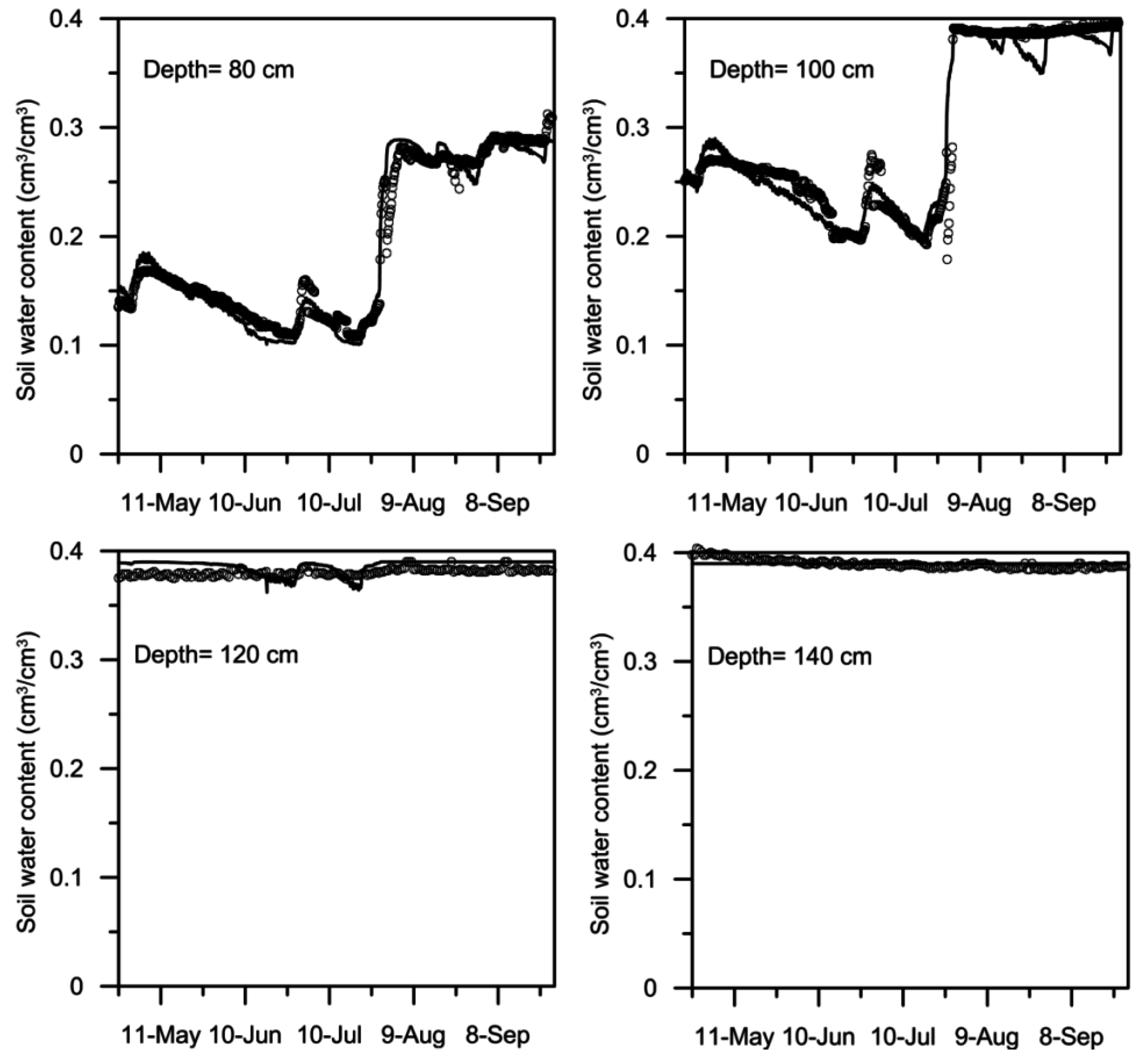
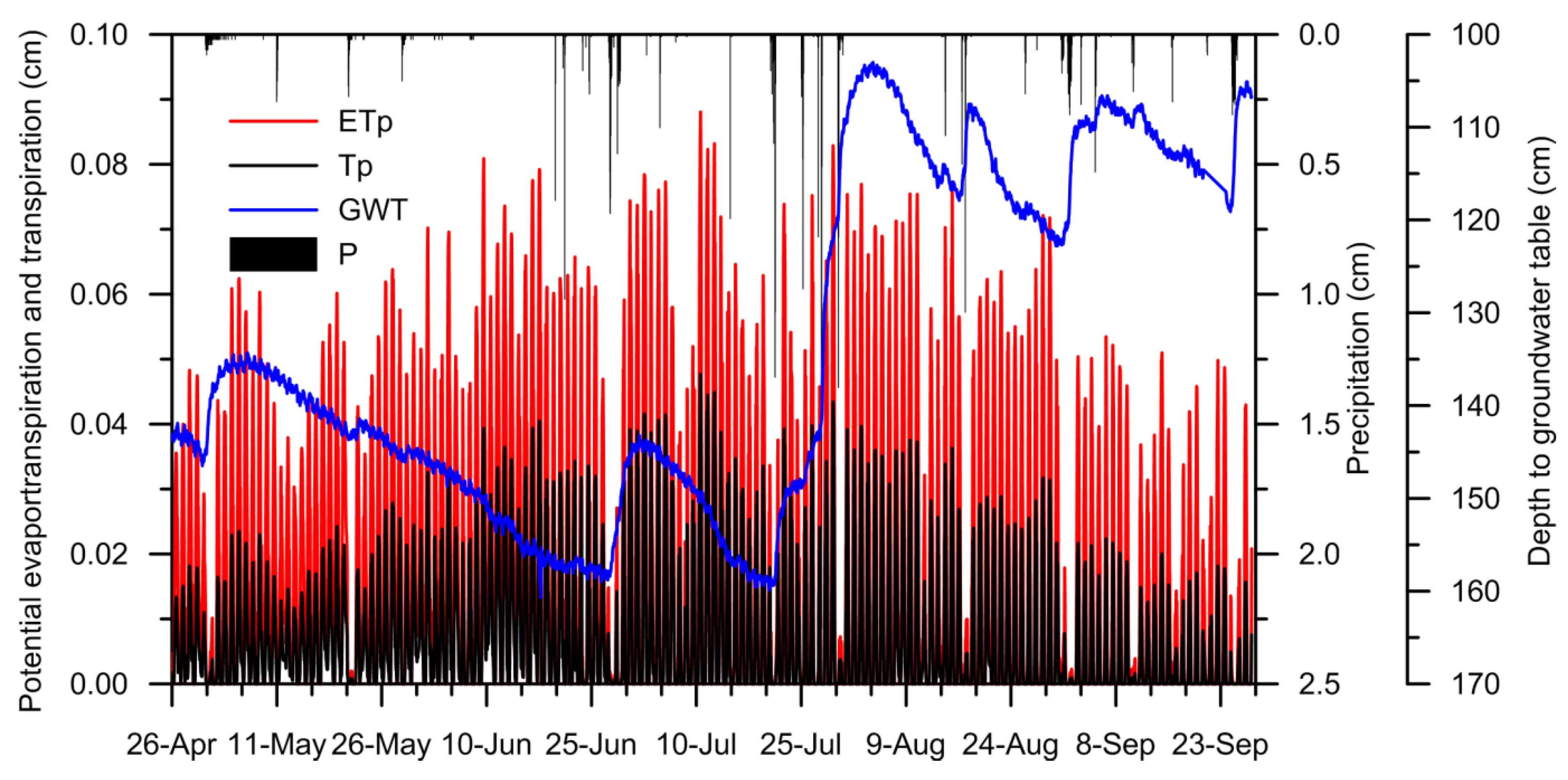
HYDRUS-1D software was used to simulate water movement at the experimental site. The soil hydraulic parameters and soil heat parameters were calibrated and validated using the soil water content and temperature data while varying the drought stress parameters h50 and p. During the model calibration period (from April 26 to July 11, 2012), in general, the soil water content gradually increased from the ground surface to the deep layers, unless rainfall occurred. Moreover, the soil water content in the shallow layers was more sensitive to rainfall than that in the deep layers. For example, a daily rainfall of 30.3 mm occurred on June 27 and triggered an increase in the soil water content at depths up to 100 cm, while after smaller rainfall events, the increase in the soil water content only reached 40 cm. During the validation period (July 12 to September 28, 2012), the soil water content increased with soil depth to groundwater. However, a large rainfall event of 41.1 mm on July 20 and subsequent rainfall resulted in an increase in the groundwater level, which thereafter remained high. The soil water content at a depth of 100 cm remained saturated until the conclusion of our experiments.
Six parameters in the van Genuchten model [
27] were calibrated using field measurements (
i.e.,
θr,
θs,
α,
n,
l, and
Ks). Calibration was performed by fitting the observed and modeled soil water contents using the Marquardt-Levenberg optimization algorithm. HYDRUS-1D ran the optimization process until it found the highest
R2 values [
21] between observed and computed soil water content.
The soil column was schematized as six soil layers based on our
in situ investigations. The parameter
Ks was determined using the inverse auger method [
35] for each layer. The remaining parameters were estimated using Rosetta [
36], a pedotransfer function that predicts hydraulic parameters from soil texture data (
Table 2).
Table 2.
Soil texture at the observation site.
Table 2.
Soil texture at the observation site.
| Depth (cm) | Sand (%) | Silt (%) | Clay (%) |
|---|
| 0–40 | 97.3 | 2.7 | 0 |
| 41–55 | 97.9 | 2.1 | 0 |
| 56–70 | 98.5 | 1.6 | 0 |
| 71–90 | 98.7 | 1.3 | 0 |
| 91–110 | 99.1 | 0.9 | 0 |
| 111–200 | 98.8 | 1.2 | 0 |
Running Hydrus-1D with Rosetta hydraulic parameter estimates and empirically determined values for saturated hydraulic conductivity in simulations produced poor agreement for the index. We therefore attempted to calibrate the soil hydraulic property model using the measured soil water content. In Equation (6), there are five unknown parameters for each layer. When using the inverse model in Hydrus-1D software, we found that fitting all five parameters in six layers at the same time tended to cause the inverse algorithm to fail. Thus, the five parameters were fitted layer by layer. This fitting method has been reported previously by other researchers [
37]. When the simulated and measured soil water contents exhibited a good agreement index, the hydraulic parameters were fixed and the drought stress parameters
h50 and
p were fitted via the measured sap flow of
S.
psammophila. Finally, the hydraulic and drought stress parameters were fixed, and the thermal parameters were fitted using the soil temperature.
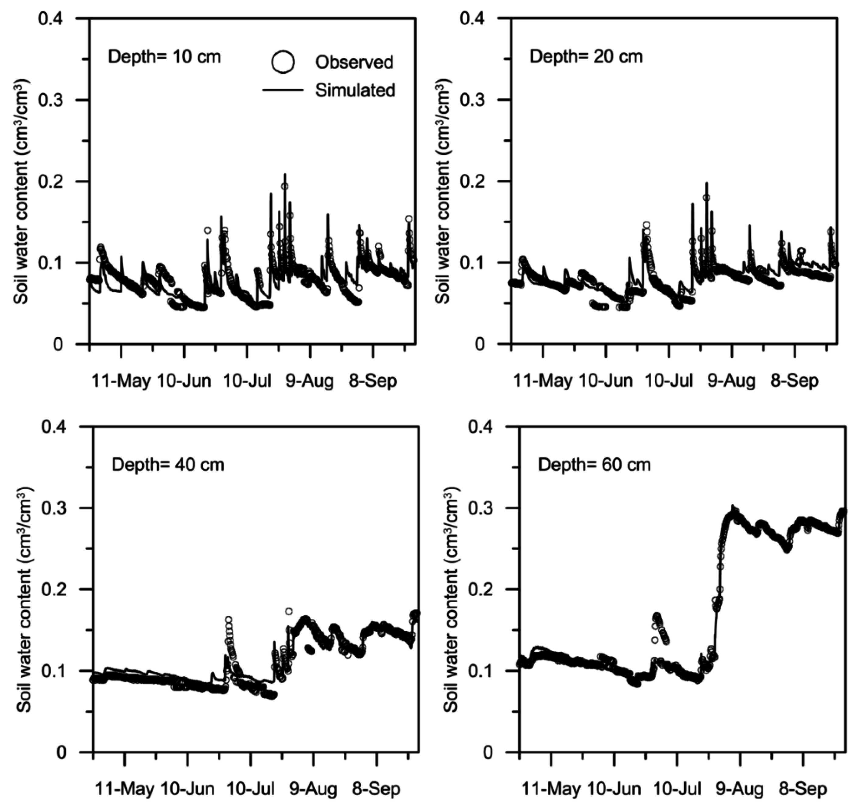
The temporal variation of the computed soil water content at the eight measurement depths during the calibration and validation periods was reasonably consistent with the field measurements at each depth (
Figure 4). We found that the parameters
α and
n were more sensitive than the other parameters.
Table 3 shows the calibrated hydraulic parameters. The statistical criteria for model calibration (Equations (13)–(16)) are summarized in
Table 4. The RMSE values were very low for both the calibration and validation periods at all measured depths. The index of agreement (
d) was very high, ranging from 0.65 to 0.96 and from 0.86 to 1.00, respectively, for the model calibration and validation periods at all depths. Generally, the calibration and validation results were acceptable. The soil water contents computed using the model captured the sharp increase in the soil water content after heavy rainfall events.
Table 3.
The calibrated parameters for the HYDRUS-1D model.
Table 3.
The calibrated parameters for the HYDRUS-1D model.
| Depth (cm) | θr (cm3·cm−3) | θs (cm3·cm−3) | α (cm−1) | n | Ks (cm·h−1) | l |
|---|
| 0–40 | 0.045 | 0.39 | 0.0550 | 2.180 | 115.70 | 0.5 |
| 41–55 | 0.075 | 0.40 | 0.0245 | 3.812 | 118.22 | 0.5 |
| 56–70 | 0.07 | 0.39 | 0.0198 | 4.873 | 113.42 | 0.5 |
| 71–90 | 0.072 | 0.29 | 0.0189 | 5.716 | 110.42 | 0.5 |
| 91–110 | 0.124 | 0.39 | 0.0295 | 2.973 | 103.02 | 0.5 |
| 111–200 | 0.065 | 0.39 | 0.01618 | 5.654 | 110.02 | 0.5 |
Reported parameter values for root-water uptake reduction by specific plants and soils range from approximately −1000 cm to −5000 cm for
h50 and from 1.5 to 3 for
p [
38]. However, especially coarse soil, such as sand, is almost completely drained of water at a fairly modest pressure head (
i.e., −300 or −400 cm). Using values for
h50 and
p that are similar to those reported in the literature caused the uptake reduction to perform essentially as a step function [
38]. On this basis, we employed an
h50 value that was considerably lower than that reported in the literature. Likewise, a larger value of
p was required to account for the steepness of the soil water retention curve. Similar to the approach reported by Zhu, Y.,
et al. [
39], we performed simulations using a range of values for
h50 and
p in an effort to calibrate the HYDRUS-1D model. As expected for Aeolian sand, the simulated water contents were not very sensitive to
h50 and
p. This finding agrees with the results of Zhu, Y.,
et al. [
39], which simulated
Populus euphratica root uptake in coarse sand soil. A comparison between simulated and measured soil water contents is presented in
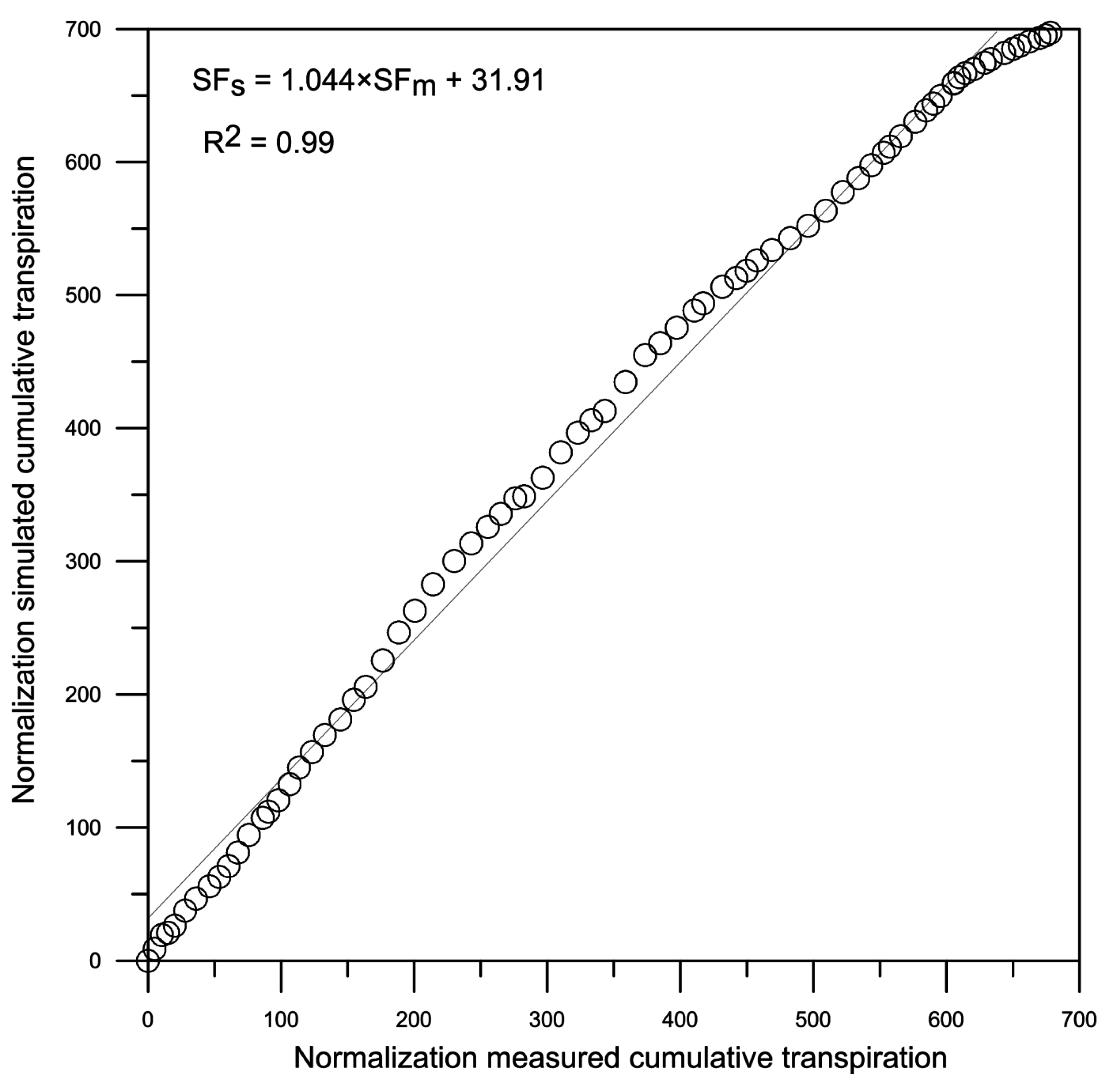
Figure 4. For our research plants, the values of
h50 and
p were found to be −630 cm and 3, respectively, from the results of fitting the predicted and measured values for transpiration (
Figure 5). It can be seen that the observed and simulated transpiration of
S.
psammophila fitted well (with
R2 = 0.99), indicating that the calibration values of
h50 and
p were acceptable.
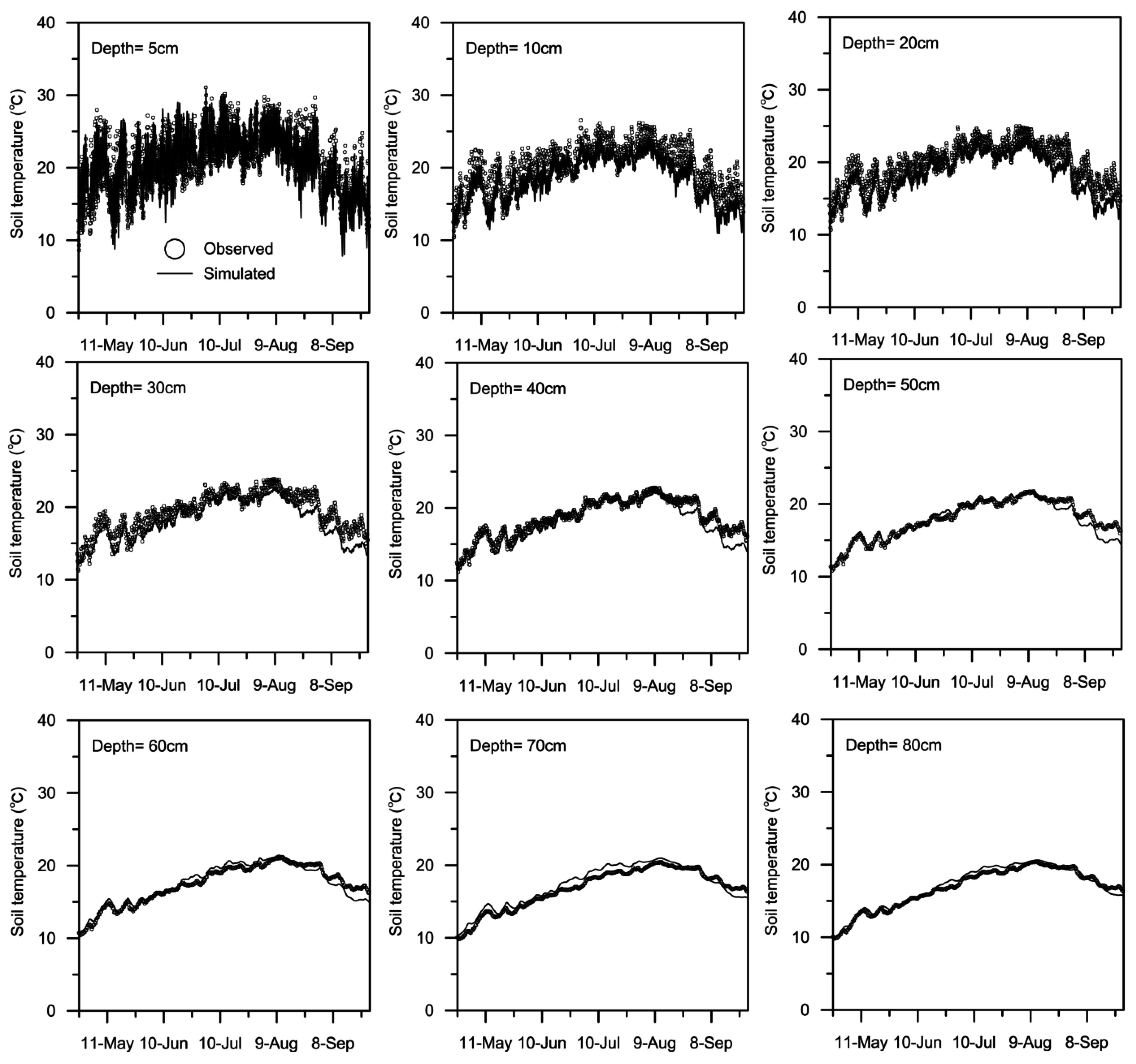
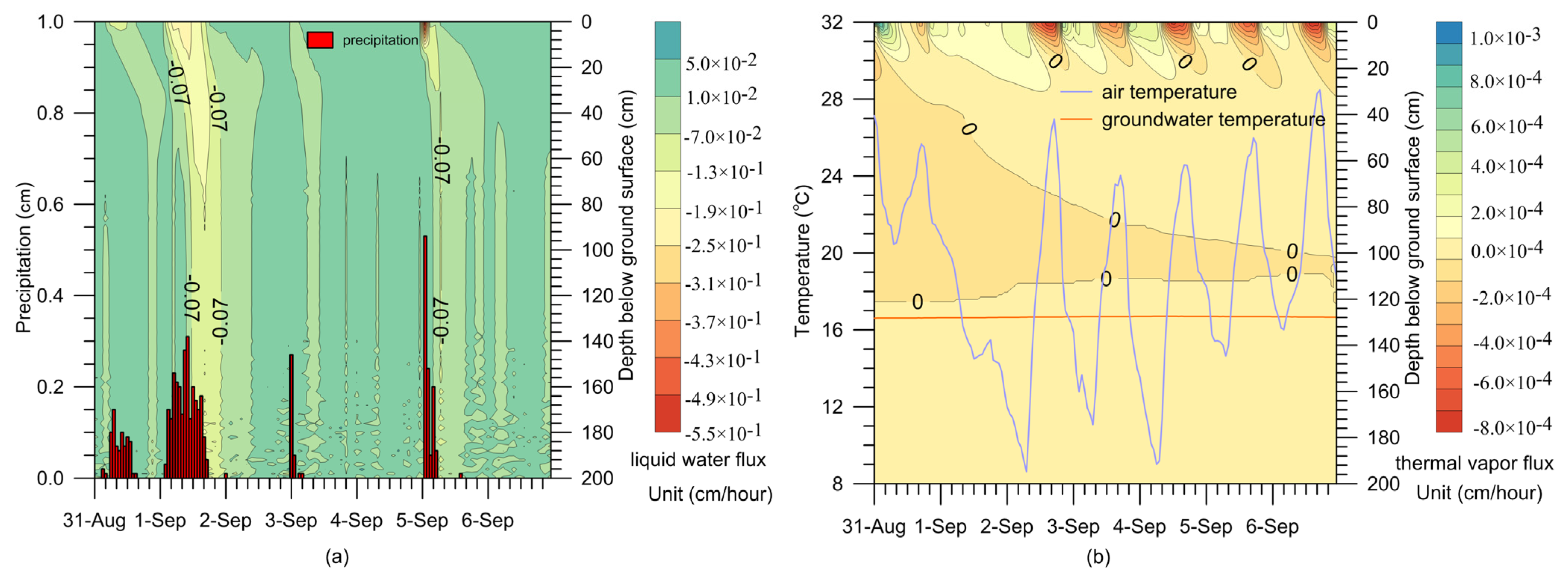
Hourly measurements of soil temperature at nine different depths reveal clear diurnal fluctuations (
Figure 6). However, both the temperature and the amplitude of the diurnal fluctuations decrease with the increase of depth because the air temperature is higher than the groundwater temperature during the measurement period spanning from 26 April to 27 September 2011, indicating downward heat transport. The temperature also exhibited seasonal variation, increasing beginning in late April, reaching the highest temperature in July and August and decreasing in September. The calibrated HYDRUS-1D model is able to simulate both seasonal and diurnal variations in soil temperature at nine different depths (
Figure 6). The statistical measures used for temperature calibration and validation are shown in
Table 5. The RMSE ranges from 0.446 °C to 2.396 °C and from 0.784 °C to 2.175 °C during the calibration and validation periods, respectively. The index of agreement (d) is larger than 0.88, during both the calibration period and the validation period, indicating a good agreement between the computed and measured soil temperatures (
Table 5).
Figure 4.
The fit of measured soil water content at eight different depths based on soil profile (points) using model-computed values (solid lines) for the calibration period (26 April to 12 July) and the validation period (13 July to 27 September).
Figure 4.
The fit of measured soil water content at eight different depths based on soil profile (points) using model-computed values (solid lines) for the calibration period (26 April to 12 July) and the validation period (13 July to 27 September).
Figure 5.
The fit of the measured (SFm) and computed (SFs) cumulative transpiration rates of the S. psammophila bush.
Figure 5.
The fit of the measured (SFm) and computed (SFs) cumulative transpiration rates of the S. psammophila bush.
Figure 6.
The fit of computed soil temperatures (solid lines) to measured temperatures (points) at nine depths in the soil profile used for calibration (26 April to 12 July) and validation (13 July to 27 September).
Figure 6.
The fit of computed soil temperatures (solid lines) to measured temperatures (points) at nine depths in the soil profile used for calibration (26 April to 12 July) and validation (13 July to 27 September).
Table 4.
Statistical measures of HYDRUS-1D model performance for simulations of volumetric water content.
Table 4.
Statistical measures of HYDRUS-1D model performance for simulations of volumetric water content.
| Simulated vs. Measured Water Content (cm3·cm−3) |
|---|
| Calibration (cm) | Validation (cm) |
|---|
| depth | 10 | 20 | 40 | 60 | 80 | 100 | 120 | 140 | 10 | 20 | 40 | 60 | 80 | 100 | 120 | 140 |
| N | 1848 | 1848 | 1848 | 1848 | 1848 | 1848 | 1848 | 1848 | 1859 | 1859 | 1859 | 1859 | 1859 | 1859 | 1859 | 1859 |
| a | 0.03538 | 0.019486 | 0.046836 | −0.01887 | −0.01928 | 0.019124 | 0.28803 | 0.386439 | 0.03538 | 0.019767 | 0.025305 | −0.00255 | 0.00503 | 0.048224 | −0.06376 | 0.390254 |
| b | 0.617928 | 0.740785 | 0.546443 | 1.194489 | 1.132598 | 0.915269 | 0.256591 | 0.008968 | 0.617928 | 0.868301 | 0.801304 | 1.009043 | 0.981768 | 0.855417 | 1.180737 | −0.00073 |
| RMSE | 0.009 | 0.008 | 0.009 | 0.005 | 0.00 | 0.012 | 0.009 | 0.005 | 0.009 | 0.008 | 0.003 | 0.000 | 0.015 | 0.036 | 0.007 | 0.003 |
| RMSEs | 0.006573 | 0.003 | 0.008 | 0.003 | 0.003 | 0.002 | 0.007 | 0.004533 | 0.006573 | 0.004841 | 0.004788 | 7.18 × 10⁻⁵ | 0.001354 | 0.017426 | 0.00535 | 0.003289 |
| RMSEu | 0.006573 | 0.007 | 0.004 | 0.005 | 0.007 | 0.011 | 0.006 | 8.14 × 10⁻⁵ | 0.006573 | 0.004841 | 0.004788 | 7.18 × 10⁻⁵ | 0.014765 | 0.031006 | 0.00496 | 8.65 × 10⁻⁵ |
| d | 0.86 | 0.88 | 0.65 | 0.93 | 0.96 | 0.94 | 0.89 | 0.85 | 0.86 | 0.86 | 0.97 | 1.00 | 0.99 | 0.94 | 0.87 | 0.89 |
Table 5.
Statistical measures of HYDRUS-1D model performance for simulations of soil temperature at different soil depths.
Table 5.
Statistical measures of HYDRUS-1D model performance for simulations of soil temperature at different soil depths.
| Simulated vs. Measured Soil Temperature (°C) |
|---|
| Calibration (cm) | Validation (cm) |
|---|
| depth | 5 | 10 | 20 | 30 | 40 | 50 | 60 | 70 | 80 | 5 | 10 | 20 | 30 | 40 | 50 | 60 | 70 | 80 |
| N | 1848 | 1848 | 1848 | 1848 | 1848 | 1848 | 1848 | 1848 | 1848 | 1859 | 1859 | 1859 | 1859 | 1859 | 1859 | 1859 | 1859 | 1859 |
| a | 0.379587 | 1.209036 | 0.883048 | 0.470773 | −0.32943 | −0.20278 | −0.08195 | 0.151507 | 0.477904 | −3.406 | −3.516 | −4.168 | −4.359 | −6.509 | −8.936 | −9.418 | −8.413 | −7.49616 |
| b | 0.909248 | 0.879813 | 0.906546 | 0.928757 | 0.995939 | 1.020258 | 1.029854 | 1.04017 | 1.048278 | 1.042 | 1.075 | 1.121 | 1.144 | 1.274 | 1.427 | 1.477 | 1.455 | 1.437842 |
| RMSE | 2.396 | 1.543 | 1.282 | 1.201 | 0.735 | 0.446 | 0.524 | 0.807 | 1.185 | 2.175 | 1.741 | 1.588 | 1.426 | 1.341 | 1.645 | 0.865 | 0.784 | 0.951 |
| RMSEs | 1.882521 | 1.145 | 0.892 | 0.837 | 0.399 | 0.134 | 0.388 | 0.748926 | 1.153619 | 0.781 | 0.738 | 0.730 | 1.111 | 1.128 | 1.356 | 0.665 | 0.540 | 0.705828 |
| RMSEu | 1.882521 | 1.033 | 0.921 | 0.861 | 0.617 | 0.426 | 0.353 | 0.301853 | 0.268979 | 0.781 | 0.738 | 0.730 | 0.644 | 0.725 | 0.931 | 0.553 | 0.569 | 0.637423 |
| d | 0.91 | 0.93 | 0.94 | 0.94 | 0.97 | 0.99 | 0.99 | 0.97 | 0.94 | 0.88 | 0.89 | 0.90 | 0.90 | 0.91 | 0.82 | 0.93 | 0.92 | 0.85 |
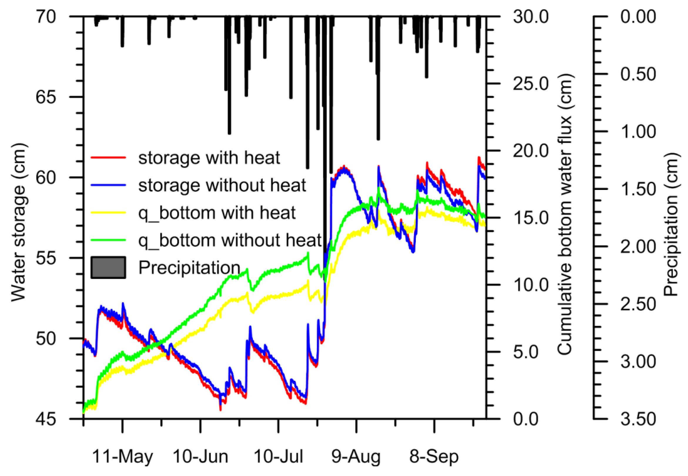
3.4. Water Storage and Bottom Flux
The change in soil water storage and bottom flux during the simulated period is shown in
Figure 9. The cumulative changes in soil water storage were 11.7 cm and 11.4 cm with and without heat flow, respectively. The heat flow thus has little influence on the change in soil water storage.
During the simulated period, the cumulative bottom flux was positive, indicating the net groundwater inflow to the soil column. The total bottom fluxes were 14.4 cm and 15.1 cm with heat flow and without heat flow, respectively. Furthermore, groundwater inflow occurs during dry days, indicating the dependency of this process on groundwater. During heavy rain, the cumulative bottom fluxes decreased, indicating groundwater recharge. For example, after 4.87 cm rain fall occurred on the June 27 and June 28, value of cumulative bottom fluxes decreased from 11.18 cm to 9.55 cm without heat and from 9.42 cm to 7.89 cm with heat, respectively. This indicated value of recharge was 1.63 cm without heat and 1.53 cm with heat, respectively.
Figure 9.
A comparison of the cumulative change in soil water storage and cumulative bottom water flux, both with and without heat flow.
Figure 9.
A comparison of the cumulative change in soil water storage and cumulative bottom water flux, both with and without heat flow.
3.7. Soil Water Contributions to Evapotranspiration
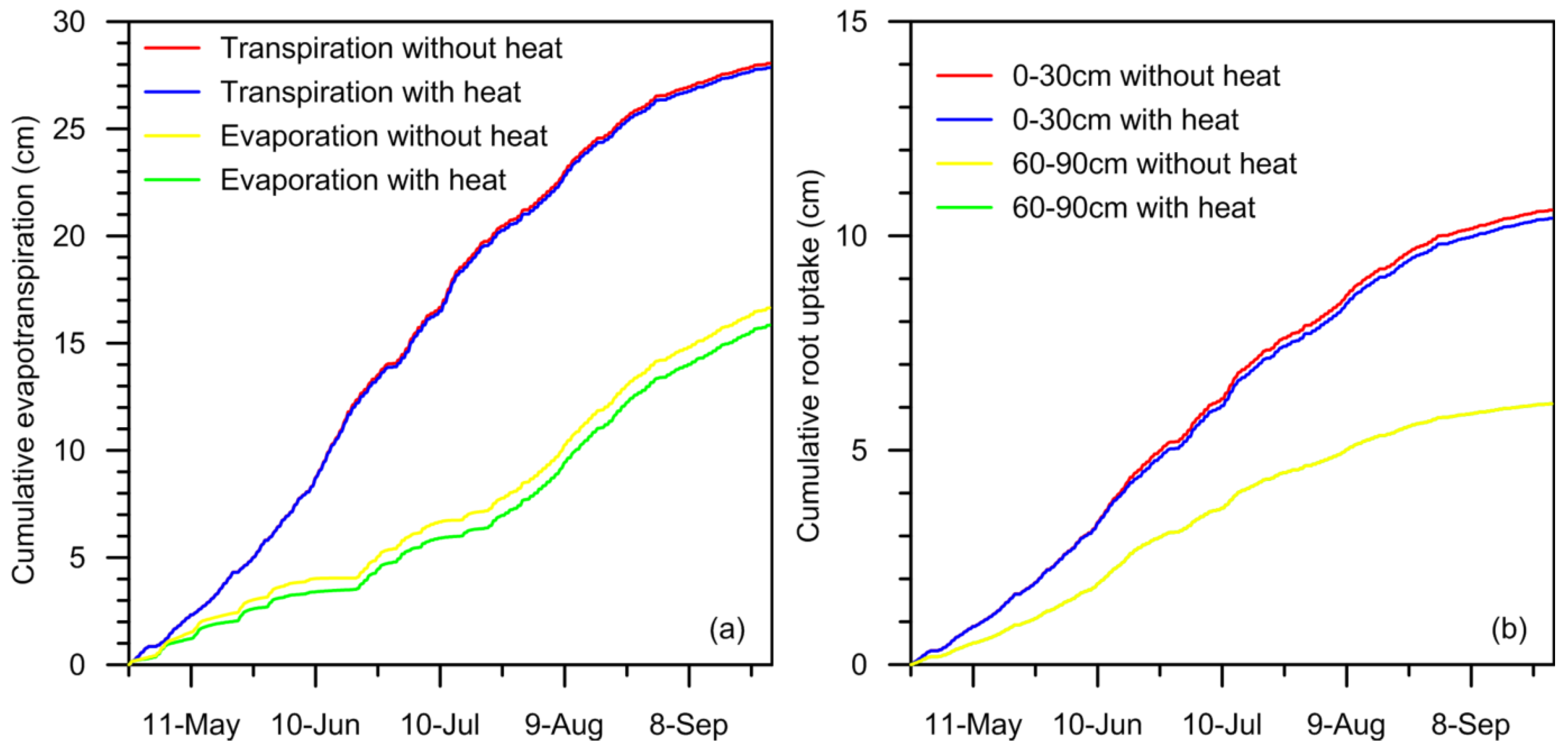
According to the previous calculations under the influence of heat flow, the soil water storage is increased by 11.7 cm. The precipitation is 41.1 cm, and the ET is 43.8 cm, including 27.9 cm of transpiration and 15.9 cm of evaporation. The total bottom water flux is 14.4 cm (upward), indicating the contribution of groundwater to the soil water balance.
To calculate the soil water contributions to evapotranspiration, the difference in the soil distribution between hydrostatic and actual conditions was used as described by Shah, N.,
et al. [
40]. When distribution of the pressure and the soil moisture reached the hydrostatic equilibrium condition, the soil acted as a vessel and the ET was supplied entirely by the groundwater without a vadose zone contribution (VZC). As the depth of the groundwater table (DWT) increased, the hydraulic connections weakened. The hydraulic connections between groundwater are lost at a rate that exceeds the upward replenishment from the saturated zone. Hence, the VZC to ET occurs in a time step of Δ
t =
ti −
ti−1 of the water content profile from hydrostatic equilibrium. Mathematically (modified from Shah N.,
et al. [
39]),
where
ETvzc is the contribution of soil water to
ET,
P is precipitation,
qbot is the calculated bottom flux, and VZC is the contribution of soil water. TSM
eq is the soil water content in the column corresponding to DWT under hydrostatic equilibrium conditions, and TSM
model is the soil water content computed from simulated by Hydrus-1D for the corresponding time.
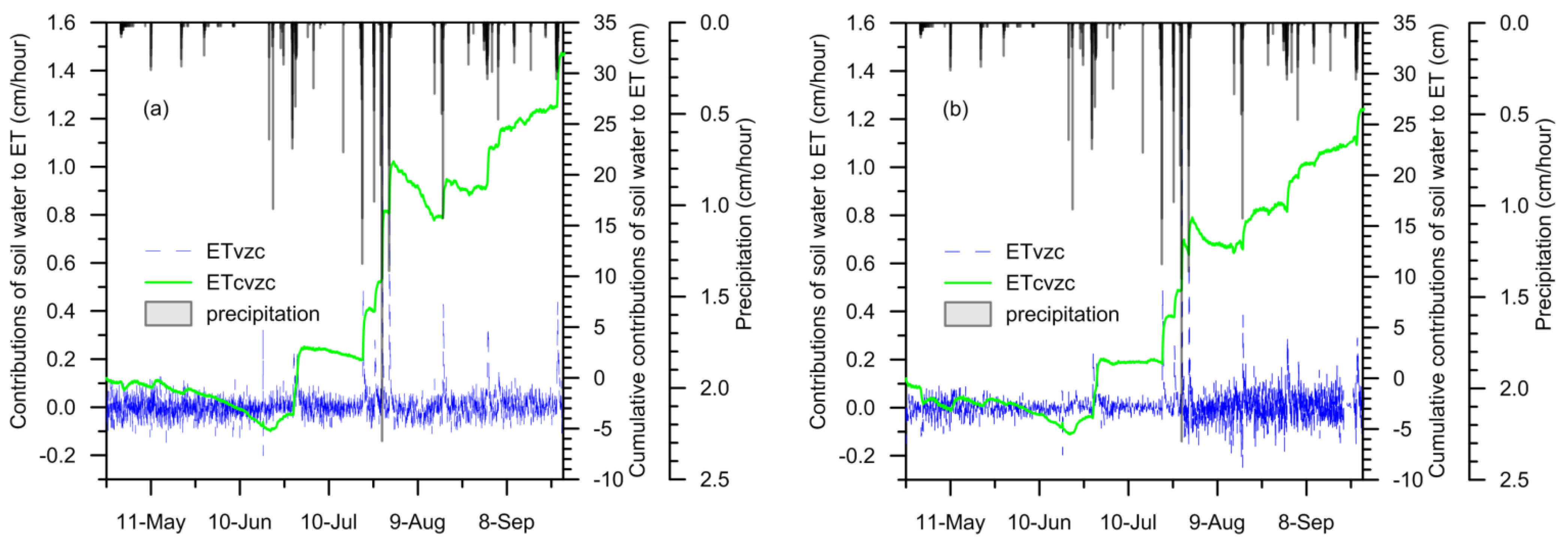
The calculated soil water contributions are shown in
Figure 13. It can be seen that during the small rainfall period, the soil is dry and the
ET is supplied by the groundwater. In contrast, after the rainfall, the soil becomes wet and the
ET mainly comes from the soil water. This result confirmed the previous research results using the soil water balance approach at the same site [
23]. However, during the simulation with heat flow, the cumulative amount of soil water and groundwater contribution to
ET are 32.0 cm and 11.8 cm, which account for 73.1% and 26.9%, respectively, of the total
ET (43.8 cm). In contrast, the cumulative soil water and groundwater contributions to
ET without heat flow are 26.6 cm and 18.2 cm, which account for 59.4% and 40.6%, respectively, of the total
ET (44.8 cm) without heat flow. The simulated results indicate that the contribution of groundwater to
ET is overestimated without considering heat flow.
Figure 13.
The contribution of soil water to ET during the simulation period (ETvzc is the soil water contribution, and ETcvzc is the cumulative contribution): (a) soil water movement with heat flow; and (b) soil water movement without heat flow.
Figure 13.
The contribution of soil water to ET during the simulation period (ETvzc is the soil water contribution, and ETcvzc is the cumulative contribution): (a) soil water movement with heat flow; and (b) soil water movement without heat flow.


