Development of Flow Forecasting Models in the Bow River at Calgary, Alberta, Canada

Abstract

River flow forecasting is critical for flood forecasting, reservoir operations, and water resources management. However, flow forecasting can be difficult, challenging and time consuming due to the spatial and temporal variability of climatic conditions and watershed characteristics. From a practical point of view, a simple and intuitive approach might be more preferable than a complex modeling approach. In this study, our objective was to develop short-term (i.e., daily) flow forecasting models in the Bow River at the city of Calgary, Alberta, Canada. Here, we evaluated the performance of several regression models, along with a newly proposed “base difference” model, by using antecedent daily river flow values from three gauge stations (i.e., Banff, Seebe, and Calgary). Our analyses revealed that using a multivariable linear regression formulated as a function of upstream gauge stations (i.e., Banff or Seebe) and the station of interest (i.e., Calgary) using antecedent flows demonstrated strong relationships (i.e., having r² (coefficient of determination) and RMSE (root-mean-square deviation) of approximately 0.93 and 14 m³/s, respectively). As such, we opted to suggest that the use of Banff and Calgary stations in forecasting the flows at Calgary could be considered as it would require a relatively lower number of gauge stations.

1. Introduction

As floods are one of the most serious natural disasters and present major societal concerns, effective flood management has always been one of the most important topics in hydrology and water resources engineering. The detrimental effects of floods, in particular extreme floods such as the 2013 flood in southern Alberta, have drawn attention to the need for more effective flood management, although the occurrence of floods cannot be prevented. Among a variety of measures for mitigating the consequences of floods, river flow forecasting, a non-structural measurement, in the short term is of great importance; whereas in the medium and long term, it is essential for reservoir operation and water resources management [1]. Therefore, depending on the use of the forecast, the lead time can be of particular concern. However, it is known that the further ahead a prediction is made, the more it is subject to lower accuracy. For flood management purposes, accurate flow forecast with several days of lead time is desired in order for there to be enough time for authorities to issue a flood warning and to allocate resources for the evacuation and relocation of the public and their valuables. Although a variety of forecasting approaches have already been formulated, developing a model to accurately forecast river flows, in particular for a river which responds to storm events quickly, has been a challenge posed to hydrologists for some time.

River flow forecasting models can be broadly classified into two general categories: process-driven models and data-driven models [1]. Process-driven models attempt to describe or represent the physical controlling processes mathematically within the watershed system, which may be achieved by combining empirical and physically based equations. In contrast, data-driven models are “black-box” in nature, as they do not require knowledge of the underlying process beforehand and are solely based on empirical equations calibrated to field data. Overall, the major differences in the two types of models are the representation of the governing processes and their data needs [2].

A rainfall–runoff model is a type of physically based model that attempts to capture the rainfall–runoff relationship. This is a difficult hydrologic phenomena to comprehend due to the complexities involved in modelling the non-linearity and tremendous spatial/temporal variability of watershed characteristics (e.g., soil type, vegetation, topography, etc.), snowpack, and precipitation patterns [3,4]. To date, various physically based models have been developed and implemented. For instance, Beven and Kirkby [5] used a topography-based hydrological model (TOPMODEL) to forecast river flow in the Crimple Beck basin in Yorkshire, England. In another study, Vieux et al. [6] utilized a physical rainfall–runoff model, called r.water.fea, which relies on conservation equations of mass and momentum for flood forecasting in the Blue River and Illinois River, USA. Similarly, Marsik and Waylen [7] used a physically-based rainfall–runoff model, called CASC2D, in the Quebrada Estero watershed in Costa Rica. Although physically based models are advantageous in terms of understanding the separate hydrological processes that govern the whole system, in many occasions the input data may be unavailable, or expensive and time consuming to collect [8]. In addition, a number of variables still need to be determined through model calibration. This makes the operation of physically-based models difficult and time consuming.

For real-time forecasting, data-driven models might be favorable, as sophisticated physical models often need tremendous amounts of data and long computational times for model calibration [8]. A data-driven model might be preferable when underlying physical mechanisms are not fully understood and if data of both input(s) and output(s) are sufficiently available to determine/establish the input–output relationship while bypassing the physical explanation of their dependence. Recently, data-driven models have been extensively used in stream flow forecasting [9,10,11,12,13,14]. The models range from straight-forward empirical models, such as regression models, to soft computing models using neural and fuzzy logic techniques. Some of such model examples are briefly described in Table 1.

Table 1. Examples of data-driven models in forecasting river flow or river water levels.

Model Type	Description
Artificial Neural Network (ANN)	ANN was used on a rainfall–runoff model to forecast daily flows on the Blue Nile river in Sudan [15]. In other studies, antecedent flows were used as input into ANN model to forecast monthly flow on the Göksudere River [12], and daily flow on the Göksu, Lamas and Ermenek Rivers [16] located in Turkey. Similarly, ANN was used to predict future groundwater levels using past observed groundwater levels in a coastal unconfined aquifer sited in the Lagoon of Venice, Italy [17].
Fuzzy Logic	Fuzzy logic was employed on a rainfall–runoff model to forecast hourly river flows for flood prediction in the Narmada River, India [18]. In other studies, daily river water levels were predicted in the Buriganga River, Bangladesh by using fuzzy logic model, in which the upstream water levels are the inputs [19].
Time Series Model	Auto-regressive (AR) and auto-regressive integrated moving average (ARIMA) models were applied to forecast monthly flows in Wabash River, Indiana, USA [20]. Noakes et al. [13] assessed the forecasting ability of ARMIA, auto-regressive moving average (ARMA) and AR models in forecasting monthly flows in 30 rivers in North and South America.
Nearest-Neighbor Method (NNM)	A comparison among ARMA, ANN, and NNM in forecasting monthly river flows using antecedent flows was conducted in the Han, Lancang, and Yangtze rivers in China [21].
Regression Model	Regression models, in which gridded observed precipitation and model-simulated snow water equivalent data were used as the predictors, were applied to forecast seasonal river flows in Sacramento River, San Joaquin River, and Tulare Lake hydrologic regions in California [9].
Adaptive Neuro Fuzzy Inference System (ANFIS)	ANFIS was used to forecast daily river flows using antecedent flows as inputs in the Great Menderes River in Turkey [10].

Table 1. Examples of data-driven models in forecasting river flow or river water levels.

Model Type	Description
Artificial Neural Network (ANN)	ANN was used on a rainfall–runoff model to forecast daily flows on the Blue Nile river in Sudan [15]. In other studies, antecedent flows were used as input into ANN model to forecast monthly flow on the Göksudere River [12], and daily flow on the Göksu, Lamas and Ermenek Rivers [16] located in Turkey. Similarly, ANN was used to predict future groundwater levels using past observed groundwater levels in a coastal unconfined aquifer sited in the Lagoon of Venice, Italy [17].
Fuzzy Logic	Fuzzy logic was employed on a rainfall–runoff model to forecast hourly river flows for flood prediction in the Narmada River, India [18]. In other studies, daily river water levels were predicted in the Buriganga River, Bangladesh by using fuzzy logic model, in which the upstream water levels are the inputs [19].
Time Series Model	Auto-regressive (AR) and auto-regressive integrated moving average (ARIMA) models were applied to forecast monthly flows in Wabash River, Indiana, USA [20]. Noakes et al. [13] assessed the forecasting ability of ARMIA, auto-regressive moving average (ARMA) and AR models in forecasting monthly flows in 30 rivers in North and South America.
Nearest-Neighbor Method (NNM)	A comparison among ARMA, ANN, and NNM in forecasting monthly river flows using antecedent flows was conducted in the Han, Lancang, and Yangtze rivers in China [21].
Regression Model	Regression models, in which gridded observed precipitation and model-simulated snow water equivalent data were used as the predictors, were applied to forecast seasonal river flows in Sacramento River, San Joaquin River, and Tulare Lake hydrologic regions in California [9].
Adaptive Neuro Fuzzy Inference System (ANFIS)	ANFIS was used to forecast daily river flows using antecedent flows as inputs in the Great Menderes River in Turkey [10].

The primary problem in the use of soft computing techniques, such as fuzzy logic and ANN, is that there is no standard set of rules on how to best implement them [22]. If a model is too simple, the solution might be far too generalized to be accurate; whereas if a model is too complex there may be insufficient generalization and its parameters could be more difficult to calibrate and interpret [23]. In the model development, a modeler has often focused on model performance, but not on the robustness and simplicity of the model itself, which could lead to over-parameterization, over-fitting, and consequently the reduction of the generalization capabilities of models. Therefore, a systematic framework, which can reduce the involvement of human objective judgments in model development, is necessary to further extend such techniques in real applications.

For a populated community, prompt forecasting, for which simple models of sufficient accuracy are indeed desirable, is crucial for reducing flood damage. Furthermore, the use of readily available data is vital for prompt forecasting. Thus, we opted to explore one of the simplest methods of analyzing data (i.e., regression analysis), which has a long history in hydrologic modeling. Nayak et al. [18] argued that increasing the model complexity by increasing the number of parameters did not enhance the model performance and suggested that simple models involving fewer parameters and simple mathematical procedures (e.g., ordinary least squares solution) would be suitable for river flow forecasting. To the authors’ best knowledge, the applicability of simple regression models for flow forecasting on the Bow River at the most populated center along the river, the city of Calgary, Alberta, Canada, has not been assessed yet. Hence, the overall objective of this paper was to develop simple and fast to implement models to forecast flows at Calgary using antecedent flows at hydrometric gauge stations in upstream of Calgary and/or at Calgary. Additionally, the specific objectives were to determine: (i) the optimal lead time forecasting the flow; and (ii) the flow gauging stations needed for more accurate forecasts.

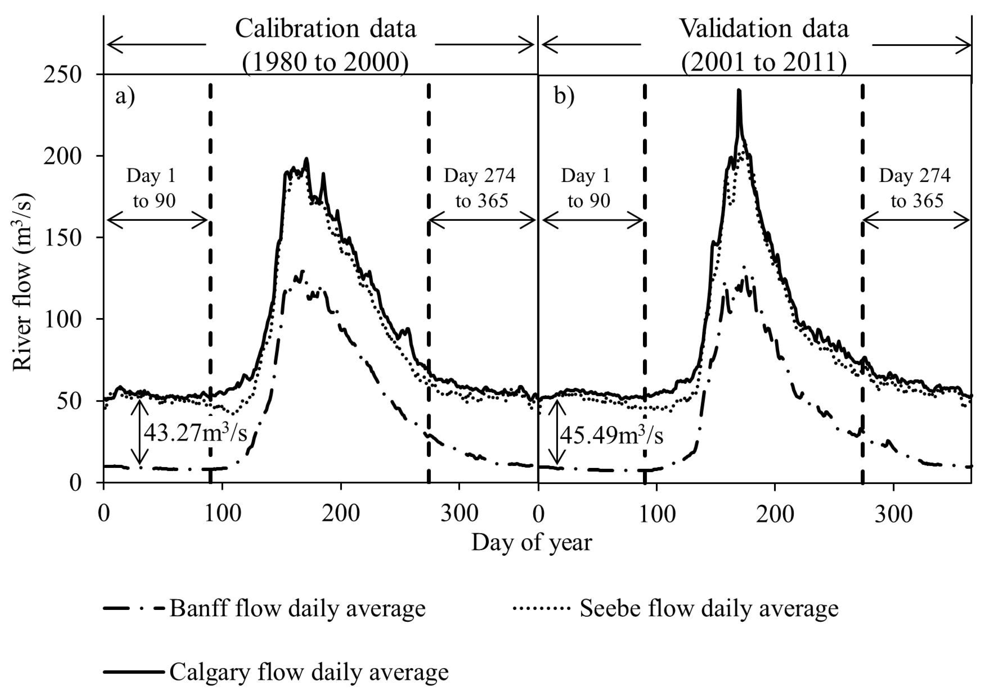
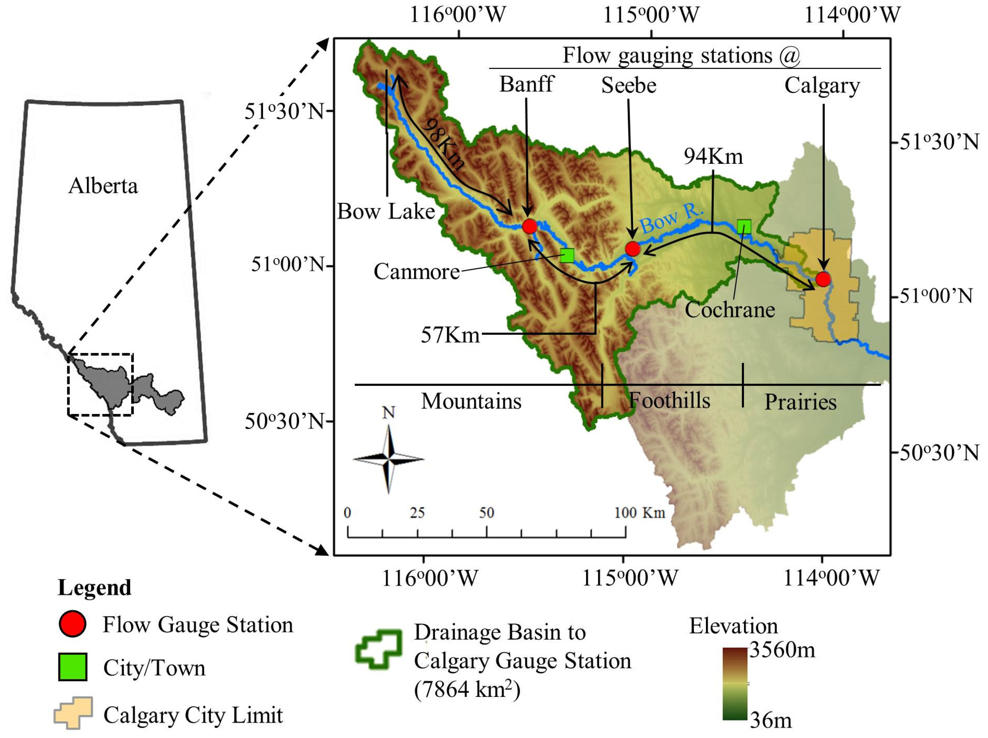
2. Study Area and Data

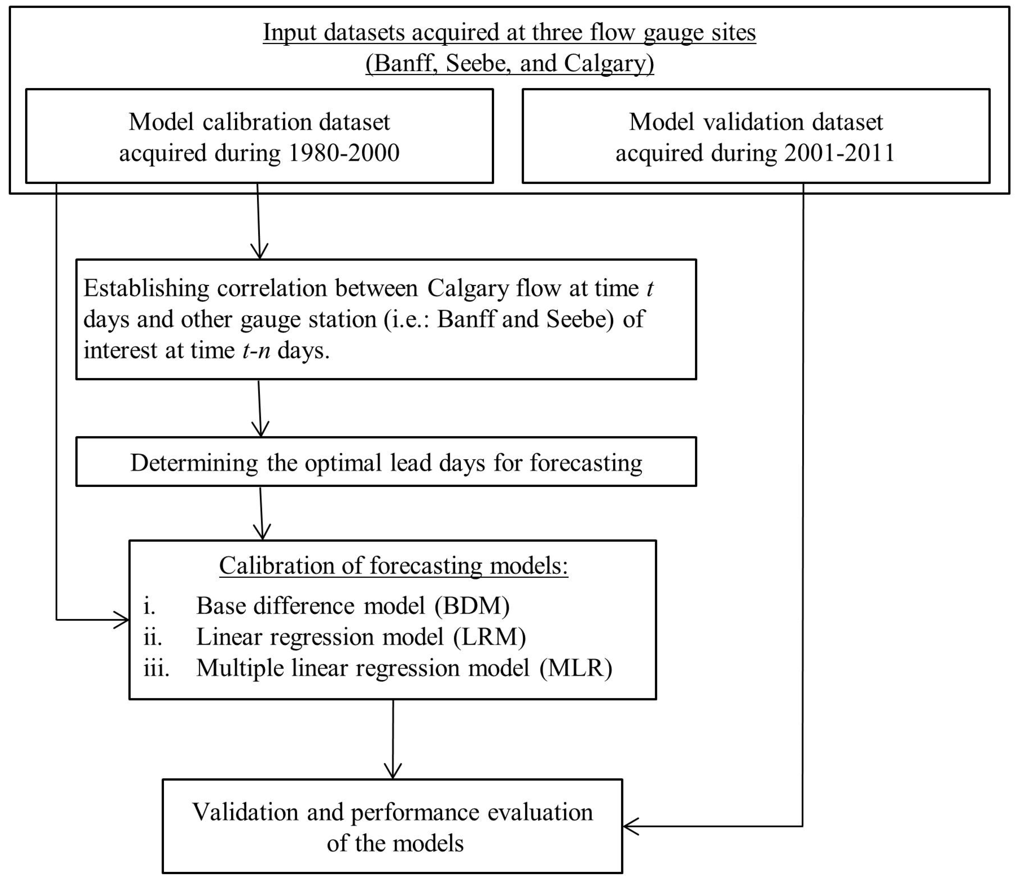
The Bow River originates from the Canadian Rockies flowing through three geographic regions: the mountains, the foothills, and the prairies. The scope of this study revolves around the upper Bow River basin, and spans from the headwaters of the Bow River, at 1920 m above sea level, to the city of Calgary, at approximately 1050 m above sea level (Figure 1). In general, the river flow is influenced by the large variations in climatic conditions that are indicative of southern Alberta, with long, cold winters and short, warm summers [24]. Winters are characterized as cold with mean temperatures of approximately −11.7, −12.4 and −11.7 °C in the coldest months of the Rocky Mountains, foothills and plains, respectively. Alternatively, summers are relatively warm with mean temperatures of approximately 11, 14.3 and 17.8 °C in the warmest months of the Rocky Mountains, foothills and plains, respectively [25]. Annual precipitation in the upper Bow River ranges from 500 to 700 mm, with about half of that amount falling as snow; while at Calgary, annual precipitation is 412 mm, with about 78% of this precipitation coming in the form of rain [24]. Climatic conditions dictate the Bow River’s water sources, which include rainfall–runoff largely from late spring to early summer, groundwater recharge which is the major water source during winter, and snowmelt that occurs in spring and summer. These spatially and temporally varying climatic conditions, occasional dry westerly Chinook winds that can cause as much as a 30 °C change in temperature [24], the relative contribution of each water source to river flow, and the spatial geological characteristic of the watershed all pose a challenge in forecasting the flow in the Bow River. Thus, a data-driven model, which can bypass the need to model the complex underlying hydrologic processes governing the flow at Calgary is indeed preferred.

Figure 1. Study area and location of the three flow gauge stations where flow data were available and used. The extent of the figure is from the origin of the Bow River to just past Calgary.

Figure 1. Study area and location of the three flow gauge stations where flow data were available and used. The extent of the figure is from the origin of the Bow River to just past Calgary.

The Bow River flows through the heart of the city of Calgary, which is home to 1.1 million [26] and can be considered one of the main commercial and cultural centers of the province of Alberta. The Bow River is prone to flooding as demonstrated in most recent major floods of 2005 and 2013 in Calgary and southern Alberta. In June 2005, city-wide heavy rains caused floods and more than 1500 Calgarians were evacuated in a state of local emergency [27]. In 2013, parts of 32 communities were evacuated affecting about 80,000 people [28].

This study focused on investigating the use of antecedent flows to forecast future flows using simple modeling approaches. Antecedent flows have been used to forecast flows or water levels in a number of previous studies [10,12,19,29]. For this study, average daily flows over 30 years from 1980 to 2011 were collected from the Water Survey of Canada (WSC) at three stations: Banff at Bow River, Seebe at Bow River, and Calgary at Bow River (Figure 1), which were chosen considering data consistency and completeness. To forecast flows at Calgary, antecedent flows at Calgary and/or at upstream gauge stations, including Banff at Bow River and Seebe at Bow River, were used as the independent variables. Although data sets including more recent observations, in particular flows during the 2013 Calgary flood, are preferable for this research objective, it should be noted that verified flow data in 2012 and 2013 had not yet been released by the WSC at all gauges stations used during the time of this study. The data was then divided into two subsets: the data from 1980 to 2000 was used in the model calibration, and the remainder was used in the model validation. Despite the fact that more gauge stations exist along the upper Bow River, it was observed that their datasets are either incomplete or not sufficiently long.

3. Methods

Figure 2 shows a schematic diagram illustrating the method developed/implemented in this study. It consisted of three major components: (i) determination of optimal lead time for flow forecasting; (ii) calibration of three different forecasting models including base difference model (BDM), linear regression model (LRM), and multiple linear regression model (MLR); and (iii) validation of the models. Among the three types of modeling approaches, the base difference model was newly proposed in this paper. The methods and procedures adopted in this paper are described in detail in the following sub-sections.

Figure 2. Schematic diagram of the methods used in this study.

Figure 2. Schematic diagram of the methods used in this study.

3.1. Determination of Optimal Lead Days for Flow Forecasting

In order to determine the optimal lead time, we conducted a correlation analysis using the calibration dataset. In the analysis, correlation coefficients were calculated between the flow at Calgary at time t day and the flow at each selected gauge stations (i.e., Banff, Seebe, and Calgary) at different time lags between 1 and 10 days. In theory, the correlation for the same (in this case Calgary station) or relatively near gauge station (i.e., Seebe station) would exhibit a stronger relationship. Thus, we put more emphasis on the further site (i.e., Banff station) and the corresponding day of the highest correlation was defined as the optimal lead time. In order to ensure a fair and even comparison among all the models developed in this paper, a single optimal lead time was determined and employed in the development of all the flow forecasting models.

3.2. Development of the Base Difference Model

There are many existing data-driven modeling methods (Table 1) that can be used or potentially used to forecast flow for this study area. However as previously highlighted, the need for simplicity and prompt forecasting still remains important in flow forecasting for flood management purposes. The newly proposed base difference model (BDM) is a simple and intuitive flow forecasting method that was developed based upon the flow characteristics observed on the Bow River in winter seasons, when flows are not significantly influenced by both snowmelt and rainfall. As a first step, we plotted the flow time-series with the calibration and validation dataset for all three gauge stations. A more or less constant offset in flow was expected between Calgary and the other two gauge stations, respectively, during late fall to early spring season (i.e., between October and March). This expectation arose from the fact that during this time period most of the precipitation would take place in the form of snow, which would consequently have little to no influence on the flow regimes. The constant offset, i.e., the average of the flow offsets from October to March between Calgary and the other gauge stations of interest calculated using Equation (1), was termed as base difference throughout this paper. The base difference along with antecedent flows was used to forecast flows at Calgary using Equation (2):

$$\overline{Q_{bd}}=\frac{{{\displaystyle \sum }}_{i=1}^n\left(Q_{cal@t}-Q_{stn@t-lead time}\right)}{n}$$

(1)

$${\tilde{Q}}_{cal@t}=Q_{stn@t-lead time}+\overline{Q_{bd}}$$

(2)

where $\overline{Q_{bd}}$ is the average base difference between Calgary and Banff/Seebe/Calgary; $Q_{cal@t}$ is the flow at Calgary at time t; $Q_{stn@t-lead time}$ is the flow at Banff/Seebe/Calgary at time t-lead time; ${\tilde{Q}}_{cal@t}$ is the forecasted flow at Calgary; n is the number of observations.

3.3. Development of the Linear Regression Models

Besides the newly proposed BDM in this study, the other simple forecasting method is linear regression. Regression analysis has been one of the most widely used techniques for analyzing data and has been employed in various disciplines [30]. Here, we expected that the linear regression model had the capabilities to yield satisfactory flow forecasts at Calgary when using antecedent flows (i.e., t-optimal lead days) at Calgary and/or upstream of Calgary, as we assumed that the independent variables are highly correlated with the dependent variable. In this study, linear regression models with one, two, and three independent variables, respectively, were created using least squares analysis. These models were developed using the calibration dataset to regress the flows at the Calgary station at time t on the flows of the other gauge station(s) at time t-lead time. Regression analyses were conducted in order to establish relations between the Calgary gauge station and: (i) Banff; (ii) Seebe; (iii) Calgary; (iv) Banff and Seebe; (v) Banff and Calgary; (vi) Seebe and Calgary; and (vii) Banff, Seebe, and Calgary; stations. Then, in the model validation, the developed regression models were applied to forecast flows at the Calgary gauge station using the validation dataset.

3.4. Validation and Evaluation of the Models

The performance of the models was evaluated by using quantitative statistical metrics, including the coefficient of determination (r²), and root mean square error (RMSE), both of which have been used in previous forecasting studies [8,10,31]. The r² indicates the goodness-of-fit; while the RMSE was selected to measure absolute errors. Please note that besides these two statistical measures, many feasible alternatives, such as the mean absolute error and the mean square relative error, can be found from the literature and that different works have used different measures to evaluate model performance. The investigation of the effects of the use of different measures for model performance evaluation is beyond the scope of this study; thus it was not assessed and discussed in this paper. The quantitative statistical metrics are calculated as follows:

$$r^2={\left(\frac{{{\displaystyle \sum }}_{i=1}^n(X-\overline{X})(Y-\overline{Y})}{\sqrt{{{\displaystyle \sum }}_{i=1}^n{(X-\overline{X})}^2}\sqrt{{{\displaystyle \sum }}_{i=1}^n{(Y-\overline{Y})}^2}}\right)}^2$$

(3)

$$RMSE= \sqrt{\frac{1}{n}{\displaystyle \sum }_{i=1}^n{(X-Y)}^2}$$

(4)

where, $Y$ is the predicted flow; $\overline{Y}$ is the mean of the predicted flows; $X$ is the observed antecedent flow; $\overline{X}$ is the mean of the observed antecedent flows; n is the number of observations.

4. Results and Discussion

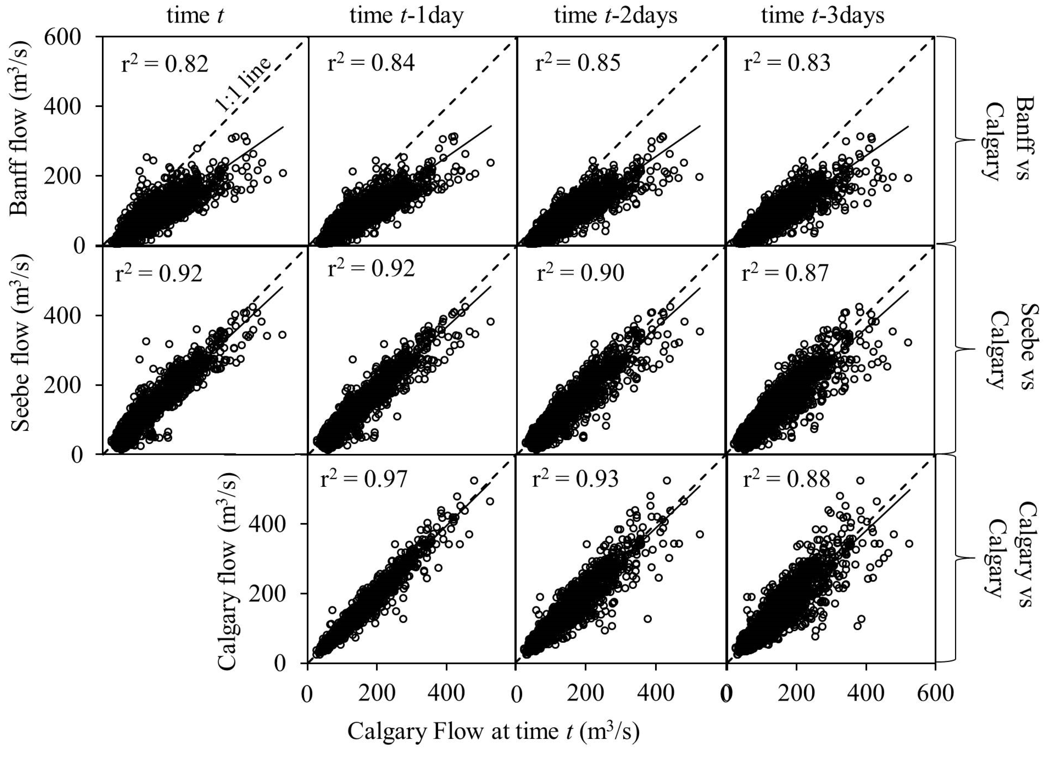
4.1. Determination of Optimal Lead Days for Flow Forecasting

Figure 3 illustrates examples of how the optimal lead time for the flow forecasting model was chosen. As expected, the graphs showed that the flow in the furthest station (i.e., Banff) had the lowest relationship (i.e., r² in between 0.82 and 0.85; top panel in Figure 3) with the flow at the prediction station (i.e., Calgary). The strongest relationships (i.e., r² in between 0.88 and 0.97) were seen using antecedent day flows at the same station as the prediction flow station (i.e., Calgary vs. Calgary; bottom panel in Figure 3). Seebe station (i.e., located between Calgary and Banff), demonstrated a middle of the pack relationship (i.e., r² in between 0.87 and 0.92; middle panel in Figure 3). Overall, the highest correlations were observed during 2, 0–1, and 1 days for Banff-Calgary, Seebe-Calgary and Calgary-Calgary stations, respectively. As previously stated, more emphasis was given on the furthest gauge station (i.e., Banff) and the corresponding day of the highest correlation (i.e., r² ≈ 0.85) was observed at 2 days. To confirm using a 2-day lead time forecasting period, a simple calculation was conducted. The average velocity measured in the Calgary reach in October of 2010 was approximately 1 m/s [32]. If we assumed this average was to be constant, then in a 2-day time period, the water would travel 172.8 km; which was close to the actual distance (i.e., ~151 km) between the two stations. In addition, for flood management perspective, longer lead time would be preferable. Considering all these factors, a time lag of 2 days was determined as the “optimal” lead time for this particular study and was employed to develop all forecasting models.

Figure 3. Determination of lead time determination for forecasting flow at Calgary using the measured flows from Banff, Seebe, and Calgary stations during the time t, t-1 day, t-2 days, t-3 days.

Figure 3. Determination of lead time determination for forecasting flow at Calgary using the measured flows from Banff, Seebe, and Calgary stations during the time t, t-1 day, t-2 days, t-3 days.

The acceptability of a forecast lead time could be relative to the size of the river and basin area to the prediction point. For example, over 90% of Bangladesh’s surface water is generated upstream of its border with respect to two major trans-boundary rivers, the Ganges and Brahmaputra, and the only reliable river flow data comes from Bangladesh gauge measurements once the rivers cross the India–Bangladesh border. Consequently, Bangladesh forecast lead times were limited to 2 or 3 days for the interior of the country and had essentially no lead time in areas close to the border [33,34]. The Ganges and the Brahmaputra basin have an area of approximately 1,087,300 and 543,400 km², respectively [35]. Together, both basins are shared among China, India, Bhutan, Nepal and Bangladesh. Yet, only 46,300 km² of the Ganges basin and 39,100 km² of the Brahmaputra lie within Bangladesh [35]. Furthermore, the Jamuna (i.e., main distributary channel of the Brahmaputra) and Padma (i.e., the main distributary of the Ganges) Rivers have an approximate length of 205 and 120 km, respectively. Our study observed a lead time of 2 days, with a drainage basin 7864 km² and a river length of 249 km from the source of the Bow River to the Calgary gauge station (see Figure 1). Although this comparison should be taken lightly, as there are many environmental factors that could influence flow forecasting besides basin size and river length, the 2-day lead time chosen for our study could be considered reasonable.

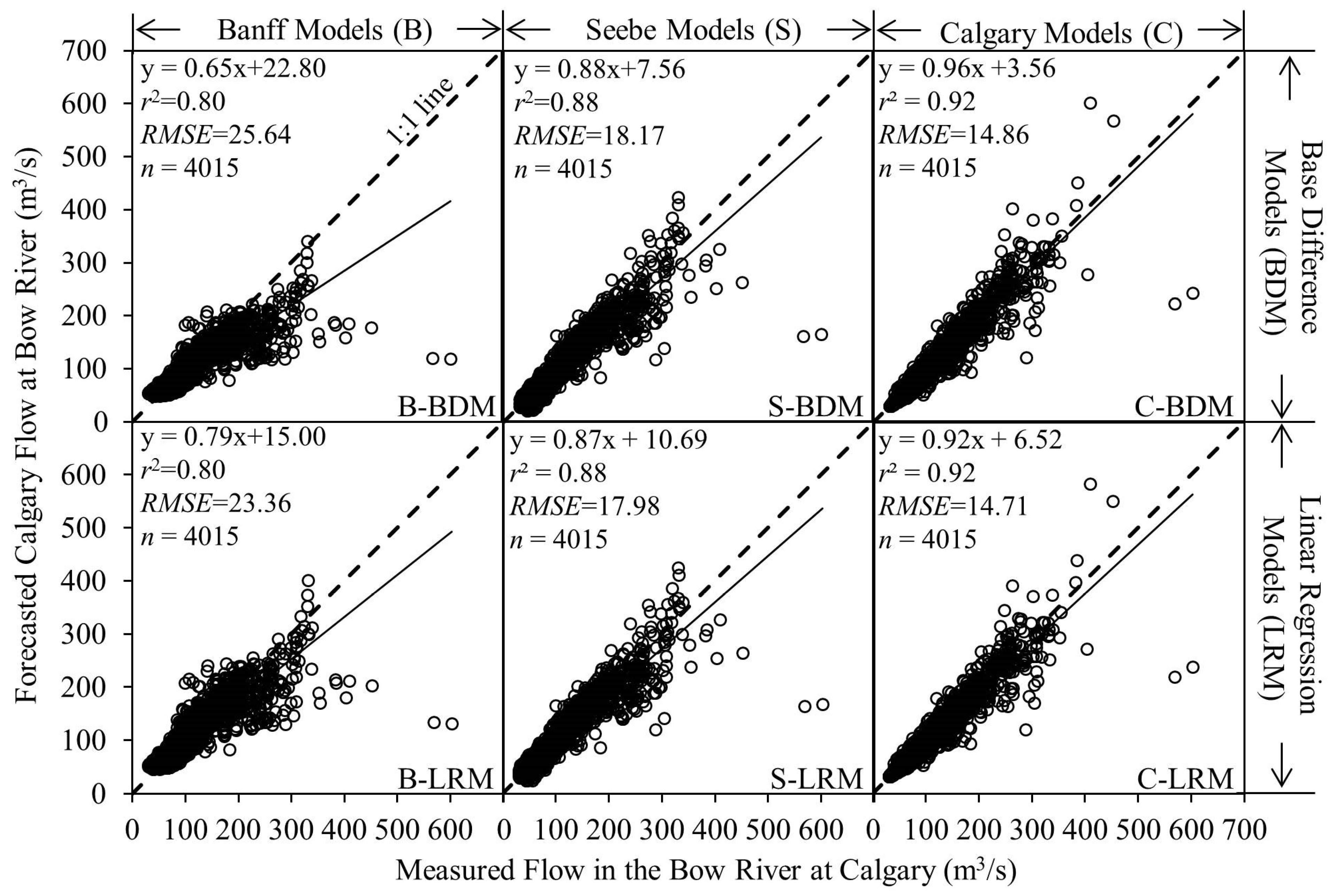
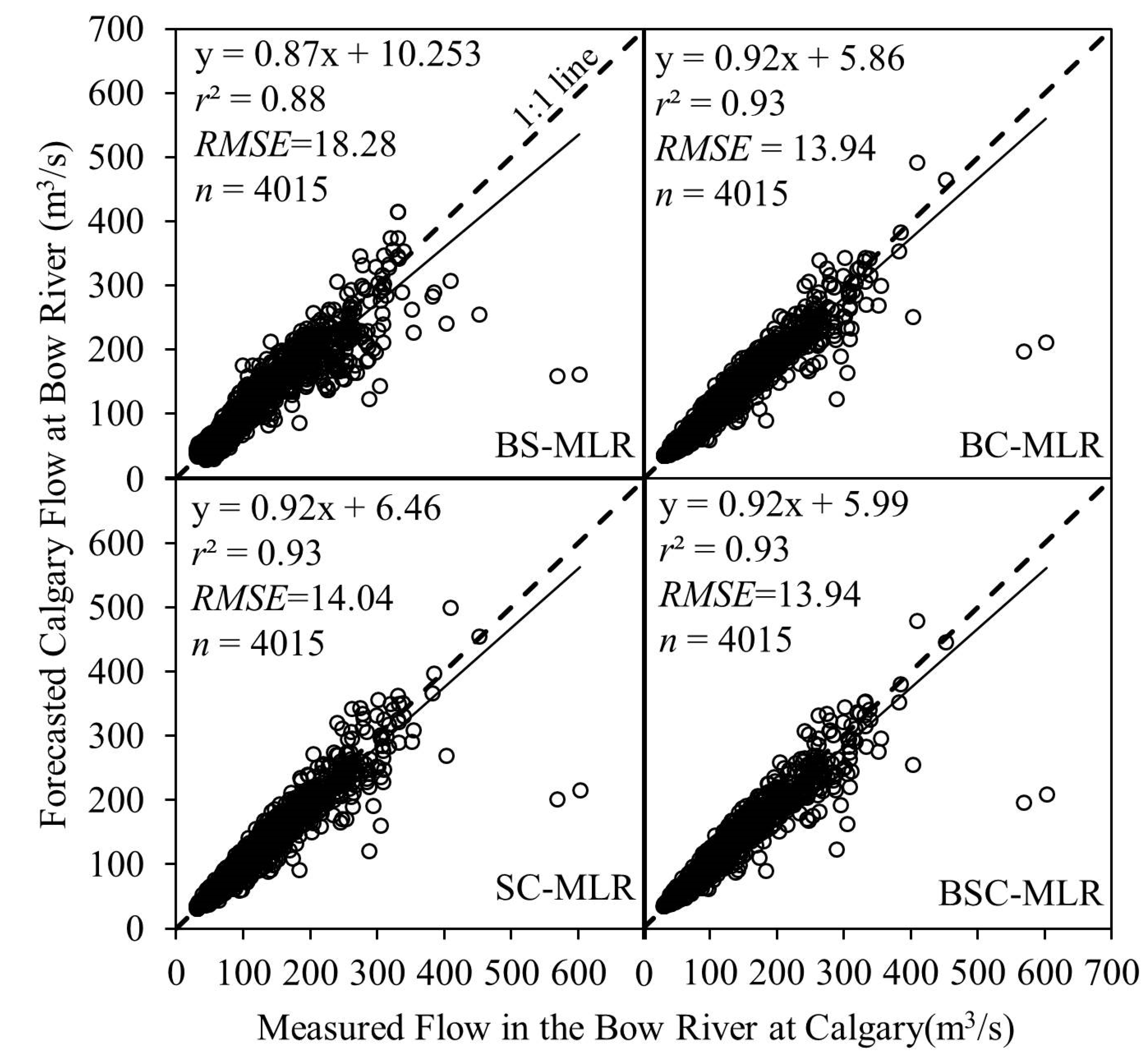
4.2. Model Calibration and Validation

Figure 4 shows average daily flows at the three gauge stations using both the calibration dataset (i.e., Figure 4a), and validation dataset (i.e., Figure 4b). During the 1980–2000 period, we observed that there was an almost constant offset (i.e., 43.27 m³/s) between Banff and Calgary within the day of year 1–90 (i.e., 1 January to 31 March) and 174–365 (i.e., 1 October to 31 December). Additionally, we noticed that the average daily flows between Calgary and Seebe within the same time periods were very similar with only an average offset of 3.25 m³/s (see Figure 4a). As mentioned in the Methods Section, the constant offsets between Banff and Calgary were expected during the observed time due to the cold weather causing precipitation to fall mostly in the form of snow and eventually accumulate on the ground. Thus, the flow during this time would primarily be influenced by groundwater recharge, and not rainfall or snowmelt. Finally, upon considering these constant offsets, we developed three base difference models as a function of optimal lead time of 2 days using the flows at Banff, Seebe, and Calgary gauge stations (see Table 2 for details).

Figure 4. Average daily river flow at each gauge station during the period: (a) 1980–2000 (i.e., the calibration dataset); and (b) 2001–2011 (i.e., validation dataset).

Figure 4. Average daily river flow at each gauge station during the period: (a) 1980–2000 (i.e., the calibration dataset); and (b) 2001–2011 (i.e., validation dataset).

In addition to the BDMs, we also developed both the linear regression models (LRMs) and multiple linear regression models (MLRs) models using the calibration dataset during the 1980–2000 period as a function of 2 days of optimal lead time (see Table 2 for details). It would be interesting to note that all of the developed models (that included BDMs, LRMs, and MLRs) demonstrated strong relationships (i.e., r² and RMSE were in the range of 0.84–0.94, and 13.63–24.16 m³/s, respectively). However, some LRMs and MLRs including C-LRM, BC-MLR, SC-MRL, and BSC-MLR, in which antecedent flows at Calgary were used as the independent variable or one of independent variables, produced more accurate forecasts according to the performance metrics. Overall, all regression models outperformed BDMs, which had the simplest mathematical formula; however, all BDMs produced sufficiently accurate forecasts, as r² of these models were all above 0.84. Despite the fact that in Table 2 the model comprising of all three station had the best agreements (i.e., r² and RMSE of 0.94, and 13.63 m³/s, respectively), we considered the MLR model comprising of the Banff and Calgary gauge stations as the most suitable (i.e., having r² and RMSE of 0.94 and 13.75 m3/s, respectively). This was because the inclusion of the Seebe station did not greatly improve performance, and as seen in Figure 4 the daily flow rates between Seebe and Calgary were somewhat redundant.

Table 2. Calibrated models and their performance metrics.

Model Type	Model	Model Equation	r2	RMSE
Base difference model	B-BDM	XBanff + 43.27	0.85	24.16
	S-BDM	XSeebe + 3.25	0.90	17.60
	C-BDM	XCalgary + 0.16	0.93	15.32
Single variable linear regression model	B-LRM	1.21 × XBanff + 39.84	0.85	21.87
	S-LRM	0.99 × XSeebe + 6.40	0.90	17.39
	C-LRM	0.96 × XCalgary + 3.25	0.93	15.17
Multiple linear regression model	BS-MLR	(0.26 × XBanff) + (0.80 × XSeebe) + 12.17	0.91	17.02
	BC-MLR	(0.36 × XBanff) + (0.72 × XCalgary) + 10.73	0.94	13.75
	SC-MLR	(0.36 × XSeebe) + (0.63 × XCalgary) + 2.75	0.94	14.12
	BSC-MLR	(0.27 × XBanff) + (0.16 × XSeebe)+(0.63 × XCalgary) + 8.69	0.94	13.63

Notes: Banff base difference model = B-BDM; Banff linear regression model = B-LRM; Seebe base difference model = S-BDM; Seebe linear regression model = S-LRM; Calgary base difference model = C-BDM; Calgary linear regression model = C-LRM; Banff & Seebe multiple linear regression model = BS-MLR; Banff & Calgary multiple linear regression model = BC-MLR; Seebe & Calgary multiple linear regression model = SC-MLR; Banff, Seebe & Calgary multiple linear regression model = BSC-MLR.

Table 2. Calibrated models and their performance metrics.

Model Type	Model	Model Equation	r2	RMSE
Base difference model	B-BDM	XBanff + 43.27	0.85	24.16
	S-BDM	XSeebe + 3.25	0.90	17.60
	C-BDM	XCalgary + 0.16	0.93	15.32
Single variable linear regression model	B-LRM	1.21 × XBanff + 39.84	0.85	21.87
	S-LRM	0.99 × XSeebe + 6.40	0.90	17.39
	C-LRM	0.96 × XCalgary + 3.25	0.93	15.17
Multiple linear regression model	BS-MLR	(0.26 × XBanff) + (0.80 × XSeebe) + 12.17	0.91	17.02
	BC-MLR	(0.36 × XBanff) + (0.72 × XCalgary) + 10.73	0.94	13.75
	SC-MLR	(0.36 × XSeebe) + (0.63 × XCalgary) + 2.75	0.94	14.12
	BSC-MLR	(0.27 × XBanff) + (0.16 × XSeebe)+(0.63 × XCalgary) + 8.69	0.94	13.63

Notes: Banff base difference model = B-BDM; Banff linear regression model = B-LRM; Seebe base difference model = S-BDM; Seebe linear regression model = S-LRM; Calgary base difference model = C-BDM; Calgary linear regression model = C-LRM; Banff & Seebe multiple linear regression model = BS-MLR; Banff & Calgary multiple linear regression model = BC-MLR; Seebe & Calgary multiple linear regression model = SC-MLR; Banff, Seebe & Calgary multiple linear regression model = BSC-MLR.

During the validation phase, all the developed models were used to conduct a 2-step ahead flow forecast using the independent validation dataset available during the 2001–2011 period. The results from the BDMs, LRMs, and MLRs are shown in Figure 5 and Figure 6. In Figure 5, the outcomes from BDMs and LRMs models were almost identical in terms of r² (i.e., in the range 0.80–0.92); however, differences were observed in RMSE-values (i.e., in the range: 14.86–25.64 m³/s for BDMs; and 14.71–23.36 m³/s for LRMs). In Figure 6, all the MLR models performed quite well with r² and RMSE in the range of 0.88–0.93 and 13.94–18.28 m³/s, respectively. However, as seen during the calibration phase, the highest performing MLR models all included antecedent flows at the Calgary gauge station (i.e., r² and RMSE were approximately 0.93 and 14.00 m³/s, respectively). In addition, the best assumed model in calibration phase (i.e., comprising of Banff and Calgary gauge stations; see Table 2) also demonstrated very strong agreements (i.e., r² and RMSE of 0.93, and 13.94 m³/s, respectively) during validation. Please also note that there appeared to be no difference in performance between BC-MLR and BSC-MLR as both the MLRs had the same performance metrics, r² and RMSE, in model validation. Their performance in model calibration also appeared to be very similar as the same r² and very similar RMSE were reported (Table 2). Therefore, it can be concluded that given that the antecedent flows at both Banff and Calgary were used as independent variables, the further inclusion of antecedent flows at Seebe was redundant as it did not enhance the model performance. In addition, these results also illustrate that all the developed models under-estimated the observed flows statistically as the regression lines of forecasted flows on observed flows locate below the 1:1 lines (Figure 5 and Figure 6).

Figure 5. Comparisons between observed flow at Calgary gauge station and predicted flow from Banff, Seebe, and Calgary using base difference and single variable linear regression models in model validation (2001–2011).

Figure 5. Comparisons between observed flow at Calgary gauge station and predicted flow from Banff, Seebe, and Calgary using base difference and single variable linear regression models in model validation (2001–2011).

It would be worthwhile to note that our findings (in particular to the model agreements) were quite comparable and/or superior to other studies. Rezaeianzadeh et al. [29] developed a multiple linear regression model as function of accumulated rainfall with 1 and 2 days antecedent flows for predicting the maximum daily flow at the outlet of the Khosrow Shirin watershed, located in the Fars Province of Iran. Although a low r² value of 0.525 was reported, similarly to our study it was observed that the inclusion of antecedent flows resulted in much better flow forecasts in both linear and nonlinear regression analyses. In addition, Sehgal et al. [36] used traditional multiple linear regression to forecast daily flow at the mouth of the delta region of Mahanadi river basin, India. This particular multiple linear regression model, which included antecedent flows of the gauge station under observation and two upstream gauge stations, saw a low r² value of 0.671 at a similar 2-day lead forecast time.

Based on the model development process of BDM, it can be seen that the flow contribution from snowmelt and rainfall can be isolated from baseflow, which is the major water source of the Bow River in winter seasons. Although the overall performance of the BDMs is not superior to other models developed in this study, their acceptable performance supports the rationale behind this modeling approach, which is that different hydrologic processes govern the flows in different seasons in this river. As BDM can forecast flows given known base difference, which can be obtained from flow observations over winter seasons, and flow at the upstream of the location of interest, this modeling approach is simpler and more intuitive compared to LRM and MLR, which would require observations to determine regression coefficients.

Figure 6. Comparisons between observed flow at Calgary gauge station and predicted flow using multiple linear regression models, i.e., BS-MLR, BC-MLR, SC-MLR, and BSC-MLR in model validation (2001–2011).

Figure 6. Comparisons between observed flow at Calgary gauge station and predicted flow using multiple linear regression models, i.e., BS-MLR, BC-MLR, SC-MLR, and BSC-MLR in model validation (2001–2011).

As illustrated in Table 2, the MLRs, in general, outperform all their counterpart models, LRMs and BDMs. It is not surprising that adding antecedent flow at one more flow gauge station, which is also strongly correlated to flows at Calgary, in MRLs would increase the models’ capability to explain the variation of flows at Calgary. The superior performance of MLRs and LRMs to BDMs might be attributed to the fact that the regressive relationship between flows at Calgary and the antecedent flows in the upstream gauge stations and/or at Calgary can account for the variation of flow resulting from the snowmelt and rainfall upstream of Calgary and in Calgary to a certain degree. On the other hand, the BDMs are developed based on the flow difference at two gauge stations and the antecedent flow, thus such models completely ignore effects of rainfall and snowmelt between Calgary and its upstream gauge station. However, please note that, despite their drawbacks, BDMs are overall capable of producing satisfactory forecasts as reflected by their performance metrics.

Despite the strong agreements between the observed and forecasted flows in both calibration and validation phases for the optimal model (i.e., BC-MLR), there were still small amounts of discrepancies (i.e., ~7% variations) that were not addressed. Within the validation of all the models, some outlier points at approximately 600 m³/s in the observed Calgary flow were apparent (see Figure 5 and Figure 6). This point corresponded to the flood that occurred in Calgary in June of 2005 due to heavy rainfalls. In Calgary, June 2005 had a total rainfall of 247.6 mm compared to a normal of 79.8 mm [37]. It was observed that none of the models developed in this study was able to account or predict for drastic changes from normal environmental conditions that influence the river flow, such as the heavy rainfalls experienced in June of 2005. Furthermore, if a large amount of rainfall or snowmelt suddenly would occur within the 2-day lead time period, the model prediction would be worse. The model performance in forecasting flow after extreme rainfall events using these simple modeling approaches is further recommended, such as in June of 2013 when extremely high flows at Calgary (e.g., 1700 m³/s) was recorded. As models were calibrated with 21 years of data (1980–2000), they reflected the average environmental conditions that occurred in our study area and could not deal with unusual scenarios. In order to reduce some of the variability that was not accounted for, a rainfall–runoff component would be worthwhile to consider. However, simply adding a rainfall–runoff term to a regression model was found to be inadequate in some studies (e.g., Shamseldin [38] and Rezaeianzadeh et al. [29]). Thus, we would suggest incorporating a more complex solution, which could represent the influence of rainfall and snowmelt on the flow regime spatially.

5. Concluding Remarks

In this paper, we developed simple and intuitive models to forecast 2-day ahead daily average river flow in the Bow River at the city of Calgary. These developments included BDMs, which was proposed based upon the fact that flows were more or less constant when the contribution of rainfall and snowmelt was negligible during winter seasons; and traditional regression models, both LRMs and MLRs. Although all these models produced acceptable results, using the regression models that included antecedent flow at the gauge station where flows were forecasted (Calgary) and an upstream station gave the most promising results. Moreover, significant improvement was not seen by using antecedent flows at all three gauge stations. The results from this study, especially results from BDMs, recommended the need to incorporate rainfall and snowmelt components to the models in order to capture their contribution. Although BDMs appear to be capable of producing satisfactory forecasts for the Bow River, its applicability to other rivers needs to be verified as the BDM was proposed based on flow characteristics observed from the Bow River. Statistically, all the developed models under-estimated flows; while a large discrepancy between observed and forecasted flows was obvious for extremely high flows, such as flow in 2005 flood. This implies that the models developed in this study did not successfully capture drastic environmental changes, such as high flows resulting from extreme rain events. In addition, the results, especially results from BDMs, obtained from this study recommended the need to incorporate rainfall and snowmelt components to the models in order to capture their contribution for further enhancing the accuracy in the forecast. It is speculated that the use of ground observations of meteorological variables might be questionable as the limited ground observations normally lack the capability to explain their spatial variation over a large area. Remote sensing has the potential to capture the spatial variability of meteorological variables in a watershed which makes it very promising in flow forecasting from this point of view. Finally, we believe that our outcomes would build a solid foundation as to compare other models that might be used in the Bow River to forecast river flows at the city of Calgary.

References

1. Wang, W. Stochasticity, Nonlinearity and Forecasting of Streamflow Processes; IOS Press: Amsterdam, The Netherlands, 2006. [Google Scholar]
2. Shrestha, R.R.; Nestmann, F. Physically based and data-driven models and propagation of input uncertainties in river flood prediction. J. Hydrol. Eng. 2009, 14, 1309–1319. [Google Scholar]
3. Beven, K. Changing ideas in hydrology—The case of physically-based models. J. Hydrol. 1989, 105, 157–172. [Google Scholar]
4. Tokar, A.S.; Markus, M. Precipitation–runoff modeling using artificial neural networks and conceptual models. J. Hydrol. Eng. 2000, 5, 156–161. [Google Scholar] [CrossRef]
5. Beven, K.J.; Kirkby, M.J. A physically based, variable contributing area model of basin hydrology/un modèle à base physique de zone d'appel variable de l'hydrologie du bassin versant. Hydrol. Sci. Bull. 1979, 24, 43–69. [Google Scholar]
6. Vieux, B.E.; Cui, Z.; Gaur, A. Evaluation of a physics-based distributed hydrologic model for flood forecasting. J. Hydrol. 2004, 298, 155–177. [Google Scholar] [CrossRef]
7. Marsik, M.; Waylen, P. An application of the distributed hydrologic model CASC2D to a tropical montane watershed. J. Hydrol. 2006, 330, 481–495. [Google Scholar] [CrossRef]
8. Chau, K.W.; Wu, C.L.; Li, Y.S. Comparison of several flood forecasting models in Yangtze river. J. Hydrol. Eng. 2005, 10, 485–491. [Google Scholar] [CrossRef]
9. Rosenberg, E.A.; Wood, A.W.; Steinemann, A.C. Statistical applications of physically based hydrologic models to seasonal streamflow forecasts. Water Resour. Res. 2011, 47. [Google Scholar] [CrossRef]
10. Firat, M.; Güngör, M. River flow estimation using adaptive neuro fuzzy inference system. Math. Comput. Simul. 2007, 75, 87–96. [Google Scholar] [CrossRef]
11. Jain, A.; Kumar, A.M. Hybrid neural network models for hydrologic time series forecasting. Appl. Soft Comput. 2007, 7, 585–592. [Google Scholar] [CrossRef]
12. Kişi, Ö. River flow modeling using artificial neural networks. J. Hydrol. Eng. 2004, 9, 60–63. [Google Scholar]
13. Noakes, D.J.; McLeod, A.I.; Hipel, K.W. Forecasting monthly riverflow time series. Int. J. Forecast. 1985, 1, 179–190. [Google Scholar] [CrossRef]
14. Wu, C.L.; Chau, K.W.; Li, Y.S. Predicting monthly streamflow using data-driven models coupled with data-preprocessing techniques. Water Resour. Res. 2009, 45. [Google Scholar] [CrossRef]
15. Shamseldin, A.Y. Artificial neural network model for river flow forecasting in a developing country. J. Hydroinform. 2010, 12, 22–35. [Google Scholar]
16. Cigizoglu, H.K. Estimation, forecasting and extrapolation of river flows by artificial neural networks. Hydrol. Sci. J. 2003, 48, 349–361. [Google Scholar] [CrossRef]
17. Taormina, R.; Chau, K.; Sethi, R. Artificial neural network simulation of hourly groundwater levels in a coastal aquifer system of the venice lagoon. Eng. Appl. Artif. Intell. 2012, 25, 1670–1676. [Google Scholar] [CrossRef]
18. Nayak, P.C.; Sudheer, K.P.; Ramasastri, K.S. Fuzzy computing based rainfall–runoff model for real time flood forecasting. Hydrol. Process. 2005, 19, 955–968. [Google Scholar] [CrossRef]
19. Liong, S.Y.; Lim, W.H.; Kojiri, T.; Hori, T. Advance flood forecasting for flood stricken bangladesh with a fuzzy reasoning method. Hydrol. Process. 2000, 14, 431–448. [Google Scholar] [CrossRef]
20. McKerchar, A.I.; Delleur, J.W. Application of seasonal parametric linear stochastic models to monthly flow data. Water Resour. Res. 1974, 10, 246–255. [Google Scholar] [CrossRef]
21. Wu, C.L.; Chau, K.W. Data-driven models for monthly streamflow time series prediction. Eng. Appl. Artif. Intell. 2010, 23, 1350–1367. [Google Scholar]
22. Yonaba, H.; Anctil, F.; Fortin, V. Comparing sigmoid transfer functions for neural network multistep ahead streamflow forecasting. J. Hydrol. Eng. 2010, 15, 275–283. [Google Scholar] [CrossRef]
23. Abrahart, R.J.; Anctil, F.; Coulibaly, P.; Dawson, C.W.; Mount, N.J.; See, L.M.; Shamseldin, A.Y.; Solomatine, D.P.; Toth, E.; Wilby, R.L. Two decades of anarchy? Emerging themes and outstanding challenges for neural network river forecasting. Prog. Phys. Geogr. 2012, 36, 480–513. [Google Scholar]
24. Bow River Basin State of the Watershed Summary. 2010. Available online: http://www.brbc.ab.ca/index.php/resources/publications/our-publications (accessed on 13 November 2014).
25. Natural Regions Commitee. Natural Regions and Subregions of Alberta. Available online: http://www.albertaparks.ca/media/2942026/nrsrcomplete_may_06.pdf (accessed on 13 November 2014).
26. Statistics Canada, 2012. Calgary, Census Profile. Available online: http://www12.statcan.gc.ca/census-recensement/2011/dp-pd/prof/index.cfm?Lang=E (accessed on 10 November 2014).
27. Flooding in Calgary. Available online: http://www.calgary.ca/UEP/Water/Pages/Flooding-and-sewer-back-ups/Flooding-and-Sewer-Back-Ups.aspx (accessed on 13 November 2014).
28. Calgary 2013 flood—Fast facts. Available online: http://www.calgary.ca/General/flood-commemoration/Pages/Media/Media-Relations-Response-June-20-21.aspx (accessed on 13 November 2014).
29. Rezaeianzadeh, M.; Tabari, H.; Arabi Yazdi, A.; Isik, S.; Kalin, L. Flood flow forecasting using ANN, ANFIS and regression models. Neural Comput. Appl. 2014, 25, 25–37. [Google Scholar] [CrossRef]
30. Montgomery, D.C.; Peck, E.A.; Vining, G.G. Introduction to linear regression analysis. In Wiley Series in Probability and Statistics, 5th ed.; John Wiley & Sons, Inc: Hoboken, NJ, USA, 2012. [Google Scholar]
31. Cheng, C.; Chau, K.; Sun, Y.; Lin, J. Long-term prediction of discharges in manwan reservoir using artificial neural network models. Lect. Notes Comput. Sci. 2005, 3498, 1040–1045. [Google Scholar]
32. Bow River BioSonics Pilot Survey with Water Quality Ground-truth Monitoring. Available online: http://environment.gov.ab.ca/info/library/8411.pdf (accessed 13 November 2014).
33. Biancamaria, S.; Hossain, F.; Lettenmaier, D.P. Forecasting transboundary river water elevations from space. Geophys. Res. Lett. 2011, 38. [Google Scholar] [CrossRef]
34. Hopson, T.M.; Webster, P.J. A 1–10-Day ensemble forecasting scheme for the major river basins of Bangladesh: Forecasting severe floods of 2003–07. J. Hydrometeorol. 2010, 11, 618–641. [Google Scholar] [CrossRef]
35. FAO. AQUASTAT—Ganges/Brahmaputra/Meghna Basin. Available online: http://www.fao.org/nr/water/aquastat/basins/gbm/index.stm (accessed 13 November 2014).
36. Sehgal, V.; Tiwari, M.K.; Chatterjee, C. Wavelet bootstrap multiple linear regression based hybrid modeling for daily river discharge forecasting. Water Resour. Manag. 2014, 28, 2793–2811. [Google Scholar]
37. Canada’s Top Ten Weather Stories For 2005. Available online: http://ec.gc.ca/meteo-weather/default.asp?lang=En&n=A4DD5AB5-1 (accessed 13 November 2014).
38. Shamseldin, A.Y. Application of a neural network technique to rainfall–runoff modelling. J. Hydrol. 1997, 199, 272–294. [Google Scholar] [CrossRef]