Volumetric Concentration Maximum of Cohesive Sediment in Waters: A Numerical Study

Abstract

Cohesive sediment has different characteristics compared to non-cohesive sediment. The density and size of a cohesive sediment aggregate (a so-called, floc) continuously changes through the flocculation process. The variation of floc size and density can cause a change of volumetric concentration under the condition of constant mass concentration. This study investigates how the volumetric concentration is affected by different conditions such as flow velocity, water depth, and sediment suspension. A previously verified, one-dimensional vertical numerical model is utilized here. The flocculation process is also considered by floc in the growth type flocculation model. Idealized conditions are assumed in this study for the numerical experiments. The simulation results show that the volumetric concentration profile of cohesive sediment is different from the Rouse profile. The volumetric concentration decreases near the bed showing the elevated maximum in the cases of both current and oscillatory flow. The density and size of floc show the minimum and the maximum values near the elevation of volumetric concentration maximum, respectively. This study also shows that the flow velocity and the critical shear stress have significant effects on the elevated maximum of volumetric concentration. As mechanisms of the elevated maximum, the strong turbulence intensity and increased mass concentration are considered because they cause the enhanced flocculation process. This study uses numerical experiments. To the best of our knowledge, no laboratory or field experiments on the elevated maximum have been carried out until now. It is of great necessity to conduct well-controlled laboratory experiments in the near future.

1. Introduction

Generally, sediment can be classified into two groups: non-cohesive sediment such as sand and cohesive sediment such as mud. Particles of non-cohesive sediment move individually. Sediment smaller than 63 µm is generally defined as cohesive sediment [1,2,3,4]. Cohesive sediments in waters form aggregated larger particles (so-called “flocs”) by through binding together (aggregation). The flocs disaggregate into smaller micro-flocs (breakup or disaggregation) mainly due to turbulent and internal shear [5], rather than breaking up into the single constituent grains [6]. This series of aggregation and breakup due to cohesive properties of sediment and flow turbulence is referred to as the flocculation process. The chance of particle collisions resulting in flocculation is caused by Brownian motion, different settling velocities of particles, and turbulence. From many studies (e.g., [7,8,9]), it is known that turbulent motions are the main mechanism in the flocculation process. The cohesive sediment continuously experiences changes of density and size through the flocculation process. Due to the change of density and size, the settling velocity of cohesive sediment also varies depending on many conditions such as particle properties, turbulence intensity, and sediment concentration. The settling velocity of particles is one of the most important factors in sediment suspension. Therefore, the flocculation process is of great interest when the suspension of cohesive sediment is studied. It is not simple to understand the mechanism of cohesive sediment transport because of the flocculation process.

In many studies, flocculation models are proposed under the assumption of self-similarity, the main concept of fractal theory (e.g., [6,9,10,11,12,13,14,15]). Kranenburg [12] proposes the proportional relationship between excessive density and yield strength of floc based on experimental results of [16,17]. It is known from Kranenburg [12] that the empirical proportionality constants represent the properties of material. It is also stated that the fractal dimension of floc is in the range of 1.4 (marine snow) to 2.2 (lacustrine flocs). Winterwerp [9] developed a floc growth type flocculation model. The model of Winterwerp [9] considers turbulence as the most dominant mechanism for floc aggregation and breakup. The empirical parameters of the model are calibrated with field data of van Leussen [18] and simulation results are in satisfactory agreement with the field results. Khelifa and Hill [11] propose a power law equation for the fractal dimensions of flocs by analyzing many observation results. Consequently, Khelifa and Hill [11] suggest a settling velocity formulation for floc under the assumption of variable fractal dimension, which depends on floc size whereas that of Winterwerp [9] is assumed to be constant. Son and Hsu [19] propose a floc growth type flocculation model for variable fractal dimension and yield strength of floc. The model is validated with laboratory experiments of [20,21,22]. The results show that a new model with variable fractal dimension and yield strength has the capability to simulate the temporal evolution of floc size reasonably well. As mentioned, properties of floc such as density and yield strength change as the floc size increases or decreases following the fractal geometry. This has a significant effect on suspension behavior of the floc because the size and density of the suspended matter (floc in this study) have a direct relationship with the settling velocity. The volumetric concentration is defined as the volume of suspended particles (flocs in this study) divided by the total volume of the fluid-particle mixture. The hindered settling effect is affected by the volumetric concentration of suspended matters. Thus, it is also known that the volumetric concentration plays an important role in calculating the settling velocity of flocs [23,24]. Turbulence is also affected by the volumetric concentration (see Equations (8) and (9)). Because the size and density of floc are variable through the flocculation process, the volumetric concentration also varies under the condition of constant mass concentration.

There are many methods for observing of floc concentration such as bottle sampling, pump sampling, acoustic method, and the nuclear method [4,25]. Among these, optical and laser diffraction systems are widely used in order to avoid disturbance of floc structure [26]. For example, the LISST (Laser In Situ Scattering and Transmissometry), one of the most popular instruments for floc observation, measures the volume of suspended flocs using the diffraction pattern created in a laser beam [27]. Results obtained by the LISST are analyzed under the assumption that particles are transparent spheres [28]. Through a comparative study, Mikkelsen et al. [29] find that a digital floc camera (DFC) underestimates the floc size compared to the LISST. They further conclude that an accurate measurement of floc volumetric concentration is of great importance when floc dynamics is studied. Milligan et al. [30] show the successive increase or decrease of concentration and median size of floc under tidal conditions. The study of Milligan et al. [30] focuses on the temporal variation of concentration and size rather than spatial variation, such as the vertical profile. Fox et al. [31] analyze field results measured in the Po River pro-delta using optical systems. The size of floc in an image is converted to the equivalent spherical diameter in order to estimate the volumetric concentration of suspended flocs. Fox et al. [31] find that the maximum volumetric concentration of floc is located not at the bed but above the bed. The vertical distribution of sediment mass concentration is usually represented by the Rouse profile. The Rouse profile has a continuous decrease of sediment concentration with increase in elevation from the bed. However, the volumetric concentration measured by Fox et al. [31] increases with elevation from the bed up to certain elevation. Fox et al. [31] insist that the elevated maximum of floc volumetric concentration is due to resuspension of coarse single particles near the bed under the assumption that the size of floc is larger than 125 μm. However, it is well known that the resuspension from the cohesive bed is caused mainly by aggregated flocs rather than individual particles [32]. Dey et al. [33] carry out experiments to understand the turbulence structure under the condition of sediment suspension and find an increase of turbulence intensity near the bed. The increased turbulence has a significant effect on floc breakup. Therefore, the conclusion of Fox et al. [31] is questionable and it is necessary to investigate the elevated maximum of floc volume concentration more intensively. The elevated maximum of floc volume concentration is found in the numerical study by Son and Hsu [34]. They find results of numerical experiments conducted by a one dimensional vertical (1DV) transport model incorporated with a floc growth type flocculation model which ensures mass conservation. Son and Hsu [34] find that the maximum volumetric concentration of floc is located at an elevation of 0.1 to 0.6 m above the bed whereas the mass concentration of floc has a maximum value at the bed. In the case of non-cohesive sediment in Son and Hsu [34], both the volumetric concentration and the mass concentration have maximum values at the bed. To the best of our knowledge, no numerical research except for Son and Hsu [34] has calculated the elevated maximum of volumetric concentration so far. However, no detailed discussion of the elevated maximum of volumetric concentration is provided in the study of Son and Hsu [34].

This study aims to investigate the volumetric concentration maximum of cohesive sediment using the 1DV numerical model developed by Son and Hsu [34]. The 1DV model of Son and Hsu [34] has been validated with field results (e.g., [34,35]) and has been adopted for numerical studies of cohesive sediment suspension (e.g., [36,37]). A detailed description of the sediment transport model and flocculation model are given in Section 2. In Section 3, the results of the numerical experiments are discussed. The final conclusions of this study are drawn in Section 4.

2. Methods and Model Descriptions

2.1. Flocculation Model

Son and Hsu [38] develop a floc growth type flocculation model which considers the flocculation process as a competition relationship between aggregation and disaggregation (Equation (1)). The first term and the second term on the right-hand-side of Equation (1) represent the aggregation process mainly due to collisions and the breakup process by which floc size decreases.

$$\frac{dD}{dt}=\frac{G{d}^{\mathrm{\beta }}}{\mathrm{\beta }\ln \frac{D}{d}+1}\left[\frac{c}{3{\mathrm{\rho }}_s}{k}_A^{’}{d}^{F-3}{D}^{-F+4-\mathrm{\beta }}-\frac{k_B^{’}}{3}{\left(\frac{\mathrm{\mu }G}{B_1}\right)}^q{d}^{-p+\frac{2q}{3}F}{D}^{-\mathrm{\beta }+\frac{2q}{3}(3-F)+1}{(D-d)}^p\right]$$

(1)

where $k_A^{’}$ = dimensionless empirical coefficient for efficiency of aggregation; $k_B^{’}$ = dimensionless empirical coefficients for efficiency of breakup; c = mass concentration of sediment (kg/m³); ρs = density of primary particle (kg/m³); D = diameter of floc; d = diameter of primary particle; F = three dimensional fractal dimension of floc; µ = dynamic viscosity of fluid (N∙s/m²); $B_1$ = coefficient related to the yield strength of floc (see [38], for more details); G = dissipation parameter (so-called “shear rate”, s⁻¹); and p and q = empirical coefficients. Winterwerp [9] suggests the values of p = 1.0 and q = 0.5 based on several constraints. The dissipation parameter, G, is calculated by the ratio of turbulent energy dissipation rate to kinematic viscosity ($G=\sqrt{\raisebox{1ex}{$ϵ$}\!\left/ \!\raisebox{-1ex}{$\nu $}\right.}$). It represents the collision frequency causing the aggregation and breakup of flocs. Khelifa and Hill [11] propose a power-law relationship of fractal dimension based on measurement results (Equation (2)).

$$F=\mathrm{\alpha }{\left(\frac{D}{d}\right)}^{\mathrm{\beta }}$$

(2)

In Equation (2), α and β are specified as α = 3.0 and $\mathrm{\beta }=\frac{\text{log}(F_c/3)}{\text{log}(D_{fc}/d)}$. The representative floc size (Dfc) and fractal dimension ($F_c$) are suggested to be Dfc = 2000 μm and Fc = 2.0 in the study of Khelifa and Hill [11], where 26 series of field/laboratory data from various sources are analyzed. The values of empirical parameters calibrated in this study are summarized in Table 1. This study is an idealized study. Therefore, it is important to keep the same conditions of flocculation process for all experiments. The values of empirical parameters for the flocculation model summarized in Table 1 are applied to all simulations in this study. The values of p, q, and B1 are proposed in the previous studies of Son and Hsu [38] and Winterwerp [9]. With these values, the flocculation model (Equation (1)) predicts the time evolution and equilibrium size of floc reasonably well (see Figure 1 of [38]). The efficiency coefficients ($k_A^{’}$ and $k_B^{’}$) are determined based on simulation results of this study. With values for $k_A^{’}$ and $k_B^{’}$, the floc size and the mass concentration are calculated to be D = O{10²} μm and c = {10°} kg/m³, respectively (see Figure 1 and Figure 2). These results are consistent with the previous in situ measurements (e.g., [39,40]).

Table 1. Empirical parameters of flocculation model.

Parameter	$k_A^{’}$	$k_B^{’}$	p	q	B1
Value	64.4770	4.82 × 10−3	1.0	0.5	2.63 × 10−14

Table 1. Empirical parameters of flocculation model.

Parameter	$k_A^{’}$	$k_B^{’}$	p	q	B1
Value	64.4770	4.82 × 10−3	1.0	0.5	2.63 × 10−14

Figure 1. Vertical profiles of calculated concentrations. The solid curves and the dashed curves represent results of non-cohesive sediment and cohesive sediment, respectively. (a) Mass concentration under a steady current; (b) Volumetric concentration under a steady current; (c) Mass concentration under the oscillatory flow condition; and (d) Volumetric concentration under the oscillatory flow condition.

Figure 1. Vertical profiles of calculated concentrations. The solid curves and the dashed curves represent results of non-cohesive sediment and cohesive sediment, respectively. (a) Mass concentration under a steady current; (b) Volumetric concentration under a steady current; (c) Mass concentration under the oscillatory flow condition; and (d) Volumetric concentration under the oscillatory flow condition.

Figure 2. Vertical profiles of volumetric concentration (a); size (b); and density (c) of suspended floc under a steady current. The volumetric concentration has a maximum around 0.2 m above the bed. The maximum floc size is shown at 0.23 m of elevation. The minimum density of floc is also located at the same elevation.

Figure 2. Vertical profiles of volumetric concentration (a); size (b); and density (c) of suspended floc under a steady current. The volumetric concentration has a maximum around 0.2 m above the bed. The maximum floc size is shown at 0.23 m of elevation. The minimum density of floc is also located at the same elevation.

The density of floc (${\mathrm{\rho }}_f)$ is calculated by Equation 3 [12]:

$${\mathrm{\rho }}_f={\mathrm{\rho }}_w+({\mathrm{\rho }}_s-{\mathrm{\rho }}_w){\left(\frac{D}{d}\right)}^{F-3}$$

(3)

where ρw = density of water. The relationship between the volumetric concentration of flocs (${\mathrm{\varphi }}_f$) and c is written as [41]:

$${\mathrm{\varphi }}_f=\left(\frac{{\rho }_s-{\rho }_w}{{\rho }_f-{\rho }_w}\right){\mathrm{\varphi }}_s=\left(\frac{{\rho }_s-{\rho }_w}{{\rho }_f-{\rho }_w}\right)\frac{c}{{\rho }_s}$$

(4)

where the volumetric concentration of sediment solid (volumetric concentration of primary particles), ${\mathrm{\varphi }}_s$, is linearly proportional to the mass concentration because the density of primary particles is usually assumed to be constant. The volumetric concentration is not linearly proportional to the mass concentration because the density of floc varies throughout the flocculation process [38].

2.2. Sediment Transport Model

Son and Hsu [34] propose model formulations for cohesive sediment transport by simplifying Eulerian-Eulerian two-phase equations of Hsu et al. [42]. The model of Son and Hsu [34] considers the continuous change of floc size and density. The x-directional (i.e., streamwise) flow momentum equation is written as:

$$\frac{\partial u}{\partial t}=-\frac{1}{{\mathrm{\rho }}_w}\frac{\partial p}{\partial x}+\frac{1}{{\mathrm{\rho }}_w\left(1-{\mathrm{\varphi }}_s\right)}\frac{\partial {\mathrm{\tau }}_{xz}^w}{\partial z}+\frac{\left(s_s-1\right){\mathrm{\varphi }}_s}{1-{\mathrm{\varphi }}_s}g{\text{sin}\mathrm{\alpha }}_s$$

(5)

where u = x-directional flow velocity; Ss = specific gravity of primary particles; $g$ = gravitational acceleration; and αs = bed slope. In this study, the bed slope is assumed to be zero. The pressure gradient in the x-direction, $\frac{\partial p}{\partial x}$, is implemented as flow forcing in the numerical model. In Equation (5), the second term on the right-hand-side represents the gradient of fluid stress. Turbulence plays a very important role in sediment suspension and flocculation of cohesive sediment. Therefore, the fluid stress is determined by an eddy viscosity model:

$${\mathrm{\tau }}_{xz}^w={\mathrm{\rho }}_w(\nu +{\nu }_t)\frac{\partial u}{\partial z}$$

(6)

where v = kinematic viscosity of fluid; and v_t = eddy viscosity. The sum of v and v_t is defined as the effective viscosity [43]. In this study, v_t is determined by the k-ε model for cohesive sediment:

$${\nu }_t=C_{\mathrm{\mu }}\frac{k^2}{ϵ}\left(1-{\mathrm{\varphi }}_f\right)$$

(7)

where Cμ = empirical coefficient set to be 0.09 in this study following the previous study of [34]; k = turbulent kinetic energy (m2/s2); and ϵ = turbulent energy dissipation rate (m2/s3). The term, (1 − ${\mathrm{\varphi }}_f$) is shown in the equation under the assumption that turbulence does not exist within a floc. These are calculated from the turbulent energy balance equation:

$$(1-{\mathrm{\varphi }}_f)\frac{\partial k}{\partial t}={\nu }_t\left[{\left(\frac{\partial u}{\partial z}\right)}^2+{\left(\frac{\partial v}{\partial z}\right)}^2\right]+\frac{\partial }{\partial \text{z}}\left[\left(\nu +\frac{{\nu }_t}{{\text{σ}}_k}\right)\frac{\partial (1-{\mathrm{\varphi }}_f)k}{\partial z}\right]-(1-{\mathrm{\varphi }}_f)ϵ+(s_s-1)g\frac{{\nu }_t}{{\sigma }_c}\frac{\partial {\mathrm{\varphi }}_s}{\partial z}$$

(8)

$$(1-{\mathrm{\varphi }}_f)\frac{\partial ϵ}{\partial t}=C_{ϵ1}\frac{ϵ}{k}{\nu }_t\left[{\left(\frac{\partial u}{\partial z}\right)}^2+{\left(\frac{\partial v}{\partial z}\right)}^2\right]+\frac{\partial }{\partial \text{z}}\left[\left(\nu +\frac{{\nu }_t}{{\sigma }_{ϵ}}\right)\frac{\partial (1-{\mathrm{\varphi }}_f)ϵ}{\partial z}\right]-C_{ϵ2}(1-{\mathrm{\varphi }}_f)\frac{{ϵ}^2}{k}+C_{ϵ3}\frac{ϵ}{k}(s_s-1)g\frac{{\nu }_t}{{\sigma }_c}\frac{\partial {\mathrm{\varphi }}_s}{\partial z}$$

(9)

where C_ϵ1, C_ϵ2, C_ϵ3, σ_k and σ_ϵ = numerical coefficients; and σ_c = Schmidt number. The values of these numerical coefficients are summarized in Table 2 (see [34], for more details).

Table 2. Numerical coefficients of turbulence balance equations.

Coefficient	$C_{ϵ1}$	$C_{ϵ2}$	$C_{ϵ3}$	σk	σϵ	σc
Value	1.44	1.92	0.00	1.00	1.30	0.5

Table 2. Numerical coefficients of turbulence balance equations.

Coefficient	$C_{ϵ1}$	$C_{ϵ2}$	$C_{ϵ3}$	σk	σϵ	σc
Value	1.44	1.92	0.00	1.00	1.30	0.5

The governing equation for sediment solid volume concentration is calculated by an advection-diffusion process:

$$\frac{\partial {\mathrm{\varphi }}_s}{\partial t}=\frac{\partial }{\partial z}\left({\mathrm{\varphi }}_s{W}_s+\frac{{\nu }_t+\nu }{{\text{σ}}_c}\frac{\partial {\mathrm{\varphi }}_s}{\partial z}\right)$$

(10)

The first and second terms on the right-hand-side represent the advection by particle settling and diffusion by molecular and turbulent motion. The settling velocity of floc particle (W_s) is determined by Stokes’ law of settling particle:

$$W_s=\frac{1}{18\mathrm{\mu }}g{D}^2({\mathrm{\rho }}_f-{\mathrm{\rho }}_w){(1-{\mathrm{\varphi }}_f)}^4$$

(11)

The density (ρ_f) and size (D) of floc are variables in Equation (11) due to the flocculation process. Therefore, the settling velocity (W_s) also changes according to flow condition and sediment concentration.

The numerical model of this study is a time-dependent flow model. The pressure gradient term of Equation (5) is calculated by an approach of Uittenbogaard et al. [44]:

$$\frac{1}{{\rho }_w}\frac{\partial p}{\partial x}=\frac{{\tau }_s-{\tau }_b}{{\rho }_{w}h}+\frac{U(t)-U_0(t)}{T_{rel}}$$

(12)

where U(t) = computed depth-averaged flow velocity; U₀(t) = prescribed depth-averaged flow velocity; τ_s = surface shear stress set to be zero in this study; h = flow depth; and T_rel = relaxation time set to be 2 × ∆t (time step of computation) in this study. The bottom shear stress (τ_b) is calculated by the bottom friction velocity (u_τ)

$${\mathrm{\tau }}_b(t)={\mathrm{\rho }}_w{u}_{\mathrm{\tau }}{(t)}^2$$

(13)

$$u_{\mathrm{\tau }}(t)={|{\mathrm{\tau }}_0(t)|}^{1/2}$$

(14)

where τ₀ = shear stress at the bottom (see [45] for more details).

For the bottom boundary condition, the continuous erosion formulation is used (e.g., [19]) and the upward erosion flux (E) is:

$$E=\text{MAX}\left[{\mathrm{\beta }}_e\left(\frac{{\mathrm{\tau }}_b(t)}{{\mathrm{\tau }}_c}-1\right),0\right]$$

(15)

where β_e = empirical erosion flux coefficient.

A no-flux boundary condition for turbulence kinetic energy is adopted in the recent model ($\raisebox{1ex}{$\partial k$}\!\left/ \!\raisebox{-1ex}{$\partial z$}\right.=0$). The bottom boundary condition for turbulence dissipation rate is calculated by a standard near-wall approximation:

$$ϵ=\frac{C_{\mathrm{\mu }}^{3/4}{k}^{3/2}}{\kappa z}$$

(16)

where $\kappa$ = von karman constant set to be 0.41 in this study.

For all simulations in this study, the height of calculation domain is fixed to be 2.0 m. The cell size is 2.0 mm. Including two ghost cells, the total number of cells is 1002. The time step is determined by Courant-Friedrichs and Lewy condition at every time step.

3. Results and Discussion

Numerical experiments are conducted here in order to study the vertical profile of volumetric concentration of flocs. The flow condition of simulation is set to be 0.5 m/s of depth-averaged velocity (uavg) in most simulation cases of this study based on in situ measurements of Fox et al. [31]. In the study of Fox et al. [31], the volumetric concentration has a maximum above the bed (not on the bed) when uavg is about 0.5 m/s. In many cases, the cohesive bed has a variable critical shear stress mainly due to consolidation. However, the critical shear stress (τc) of cohesive bed is set to be 0.17 kPa here following the previous study of Hsu et al. [42] and Son and Hsu [34,36] because we like to exclude the effect of erodibility parameters (e.g., [8]) on behaviors of sediment suspension. In the case of non-cohesive sediment simulation, the critical shear stress is calibrated to fit the depth-averaged concentration of non-cohesive sediment to that of cohesive sediment. The density and size of non-cohesive sediment are also determined using the average values of cohesive sediment results in order to investigate the effect of flocculation on ${\mathrm{\varphi }}_f$ under the similar conditions of flow and suspension. All results discussed in this study are obtained after the equilibrium state is achieved.

The numerical experiments are carried out under two different flow conditions: pure current condition of u_avg = 0.5 m/s and oscillatory flow replicating U-tube experiments. The oscillatory flows are defined by the free-stream flow velocity (U) for simplicity (Equation (17)). The oscillatory flow conditions are symmetric in this study.

$$U(t)=u_{amp}\text{sin}\left(\frac{2\pi t}{T}\right)$$

(17)

where u_amp = orbital amplitude; T = period of oscillation; and t = time.

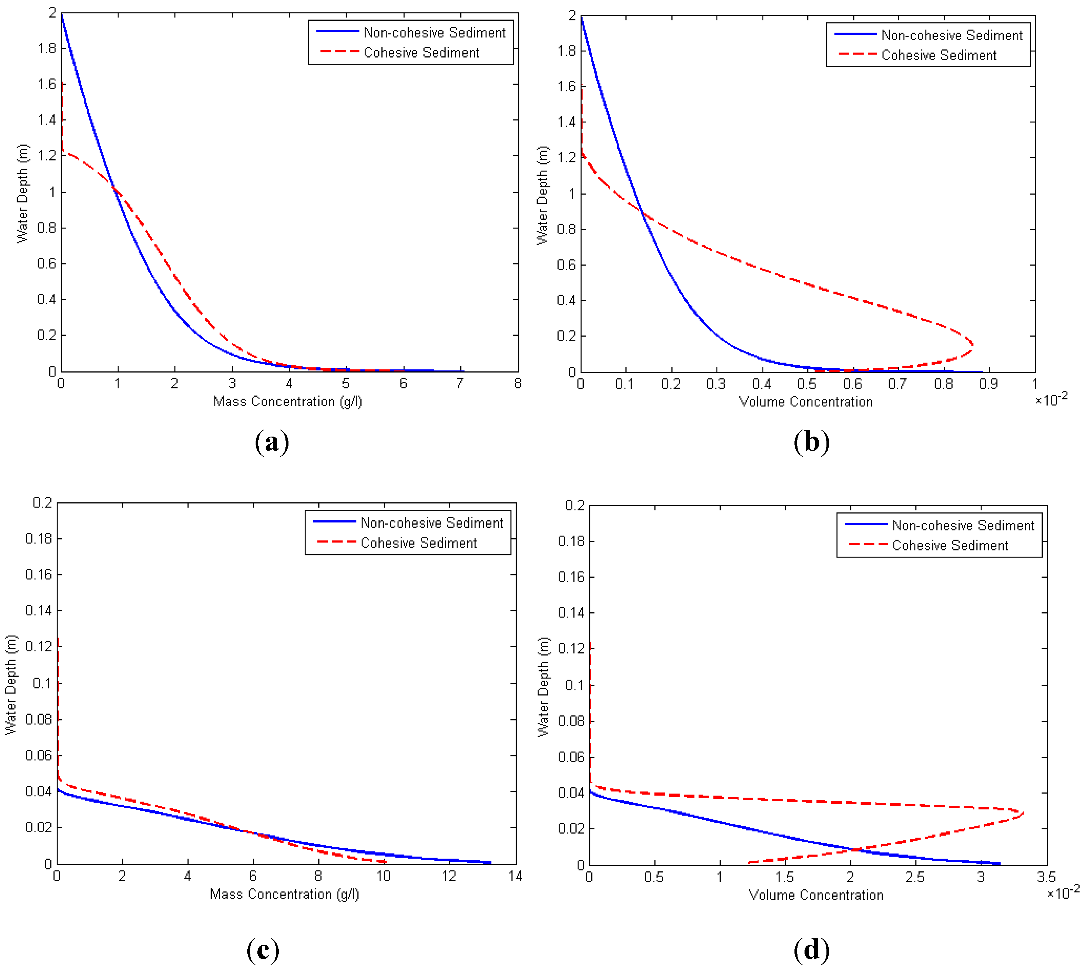
Figure 1 shows the vertical profiles of suspended sediment concentration. The solid curve and the dotted curve represent results of non-cohesive sediment and cohesive sediment, respectively. Figure 1a,b are results under the steady current condition. Figure 1c,d show the phase-averaged profiles under the oscillatory flow condition of u_amp = 0.5 m/s and T = 7.0 s. In simulation results of cohesive sediment under a steady current, it is seen that the mean size and density of flocs are 73.8 μm and 1496 kg/m³, respectively (refer to Figure 2). In the case of oscillatory flow, those are 148 μm and 1263 kg/m³. Based on the calculation result of cohesive sediment case, the density and size of non-cohesive sediment are fixed to be 73.8 μm and 1496 kg/m³ under a steady current. Under the condition of oscillatory flow, those are set to be 148 μm and 1263 kg/m³. The depth-averaged mass concentrations in the cases of current and oscillatory flow are 1.166 kg/m³ and 0.1116 kg/m³, respectively. The mass concentration profile of non-cohesive sediment continuously decreases in the vertical direction. The mass concentration of cohesive sediment under a steady current has a clear lutocline around 1 m above the bed. The volumetric concentration profile of non-cohesive sediment is linearly proportional to the mass concentration because the density of sediment is constant. It is found in Figure 1b that the profile of ${\mathrm{\varphi }}_f$ for cohesive sediment shows a peak value around 0.2 m above the bed under a steady current. ${\mathrm{\varphi }}_f$ of cohesive sediment increases in the range of 0 m to 0.2 m from the bed whereas the mass concentration of cohesive sediment shows the typical shape of a Rouse profile (see Figure 1a). The sediments under the oscillatory flow condition are confined near the bed similar to sheet flow. However, the maximum value of ${\mathrm{\varphi }}_f$ exists at the elevation of 4 cm above the bed whereas that of the non-cohesive sediment exists at the bed. In Figure 1, it can be seen that the elevated maximum of ${\mathrm{\varphi }}_f$ is not caused by the type of flow condition because the elevated maximum is shown under both steady and oscillatory currents. The difference between profiles of mass and ${\mathrm{\varphi }}_f$ result from the spatial variation of floc density and size. The density of floc decreases as the size of floc increases (see Equations (2) and (3)). Thus, it is deduced that the size of floc is large and the density is low near the elevation where the maximum value of ${\mathrm{\varphi }}_f$ exists. 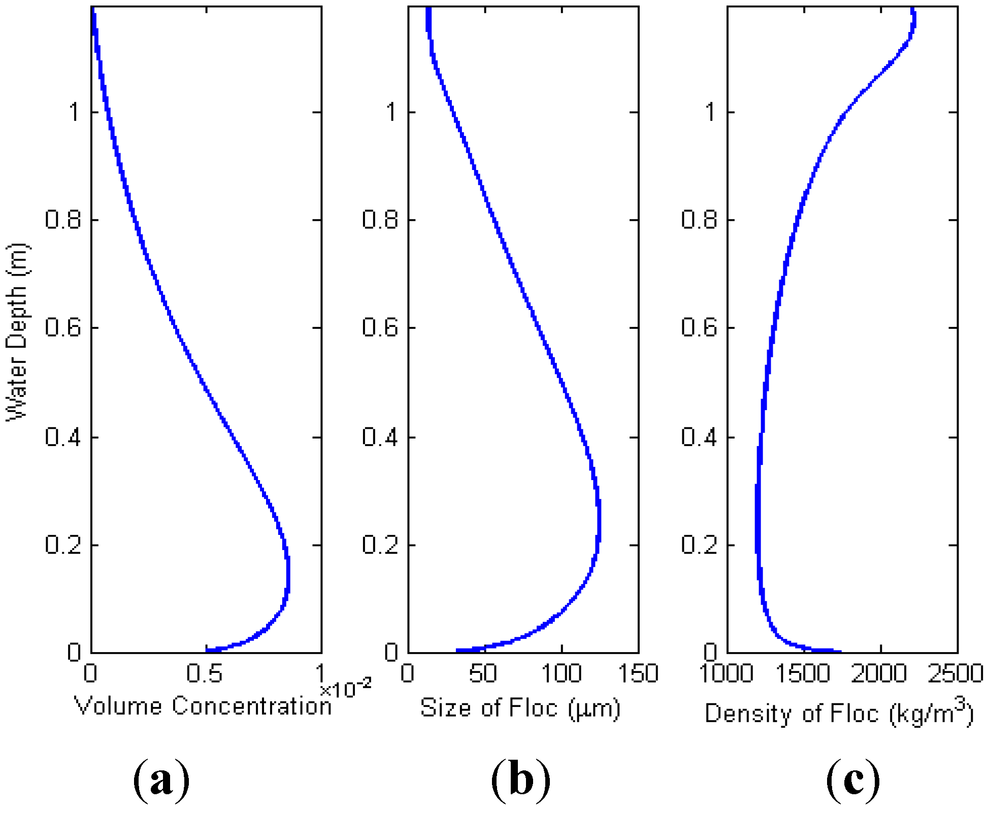Figure 2 shows the vertical profiles of ${\mathrm{\varphi }}_f$, size, and density of floc under the steady current (uavg = 0.5 m/s). As discussed above, the maximum size and the minimum density of floc are calculated near the elevation at which the maximum value of ${\mathrm{\varphi }}_f$ is located.

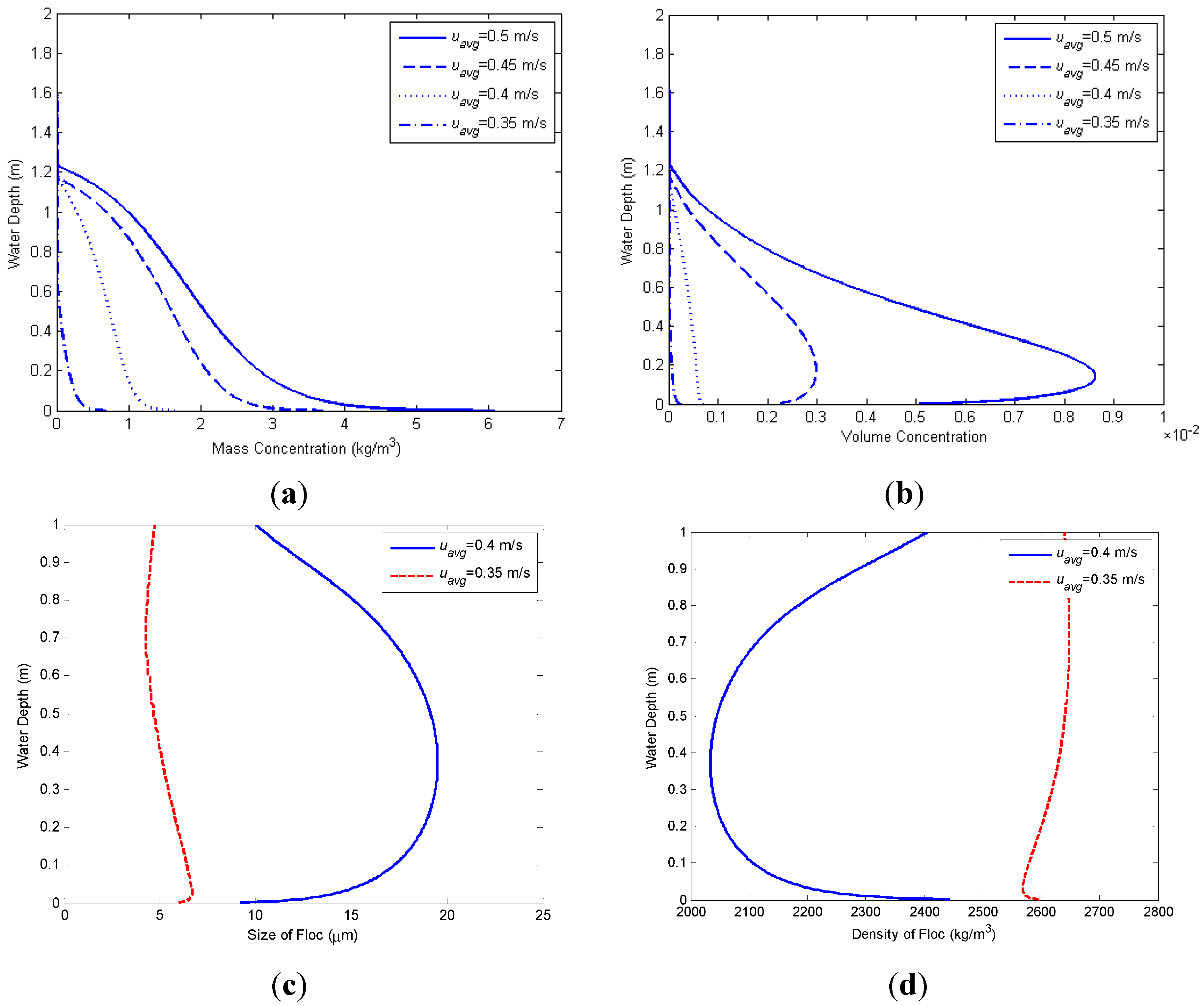
Figure 3 represents the profiles of c, ${\mathrm{\varphi }}_f$, D, and ρf under the different conditions of flow velocity. In Figure 3, it can be seen that both depth-averaged and near-bed concentrations are decreased as uavg decreases. The elevated maximum of ${\mathrm{\varphi }}_f$ is found when uavg is larger than 0.4 m/s. The profiles of ${\mathrm{\varphi }}_f$ under the conditions of uavg = 0.4 m/s and uavg = 0.35 m/s are similar to those of mass concentration. The maximum size and the minimum density of floc under the conditions of uavg = 0.4 m/s and uavg = 0.35 m/s are also located at elevations of 0.35 m and 0.03 m, respectively (see Figure 3c,d). Therefore, the near-bed maximum concentration in the cases of uavg = 0.4 m/s and uavg = 0.35 m/s is not denyed by the location of maximum floc size and the minimum floc density. The maximum floc size in the cases of uavg = 0.4 m/s and uavg = 0.35 m/s is calculated to be less than 20 μm. Compared to the size of the primary particle (4 μm), 20 μm of floc size is still small. This means that flocs have not experienced sufficient size evolution in the cases of uavg = 0.4 m/s and uavg = 0.35 m/s. As mentioned in the first paragraph of this section, ${\mathrm{\tau }}_c$ is set to be 0.17 kPa in this study. The aggregation process is affected by c (see Equation (1)). As shown in Figure 3a, c under the conditions of of u_avg = 0.4 m/s and u_avg = 0.35 m/s is relatively small compared to the cases of of u_avg = 0.45 m/s and u_avg = 0.50 m/s.

Figure 3. Vertical profiles of floc concentration under the different conditions of current velocity. (a) c under Different Conditions of u_avg; (b) ϕ_f under different conditions of u_avg; (c) D under different condition of u_avg; and (d) ρ_f under different condition of u_avg. (a) The mass concentration shows a lutocline which is the important characteristics of cohesive sediment suspension; (b) The volumetric concentration shows the elevated maximum when the velocity exceeds 0.4 m/s; (c) The maximum size of floc in the cases of u_avg = 0.40 m/s and u_avg = 0.35 m/s is also located at elevations of 0.35 m and 0.03 m (not at the bed); (d) The resulting density of floc shows the maximum values not at the bed but above the bed. In (a) and (b), the solid, dashed, dotted and dash-dotted curves represent results of u_avg = 0.50 m/s, u_avg = 0.45 m/s, u_avg = 0.40 m/s, and u_avg = 0.35 m/s, respectively. In (c) and (d), the solid and dashed curves show the results of u_avg = 0.40 m/s and u_avg = 0.35 m/s.

Figure 3. Vertical profiles of floc concentration under the different conditions of current velocity. (a) c under Different Conditions of u_avg; (b) ϕ_f under different conditions of u_avg; (c) D under different condition of u_avg; and (d) ρ_f under different condition of u_avg. (a) The mass concentration shows a lutocline which is the important characteristics of cohesive sediment suspension; (b) The volumetric concentration shows the elevated maximum when the velocity exceeds 0.4 m/s; (c) The maximum size of floc in the cases of u_avg = 0.40 m/s and u_avg = 0.35 m/s is also located at elevations of 0.35 m and 0.03 m (not at the bed); (d) The resulting density of floc shows the maximum values not at the bed but above the bed. In (a) and (b), the solid, dashed, dotted and dash-dotted curves represent results of u_avg = 0.50 m/s, u_avg = 0.45 m/s, u_avg = 0.40 m/s, and u_avg = 0.35 m/s, respectively. In (c) and (d), the solid and dashed curves show the results of u_avg = 0.40 m/s and u_avg = 0.35 m/s.

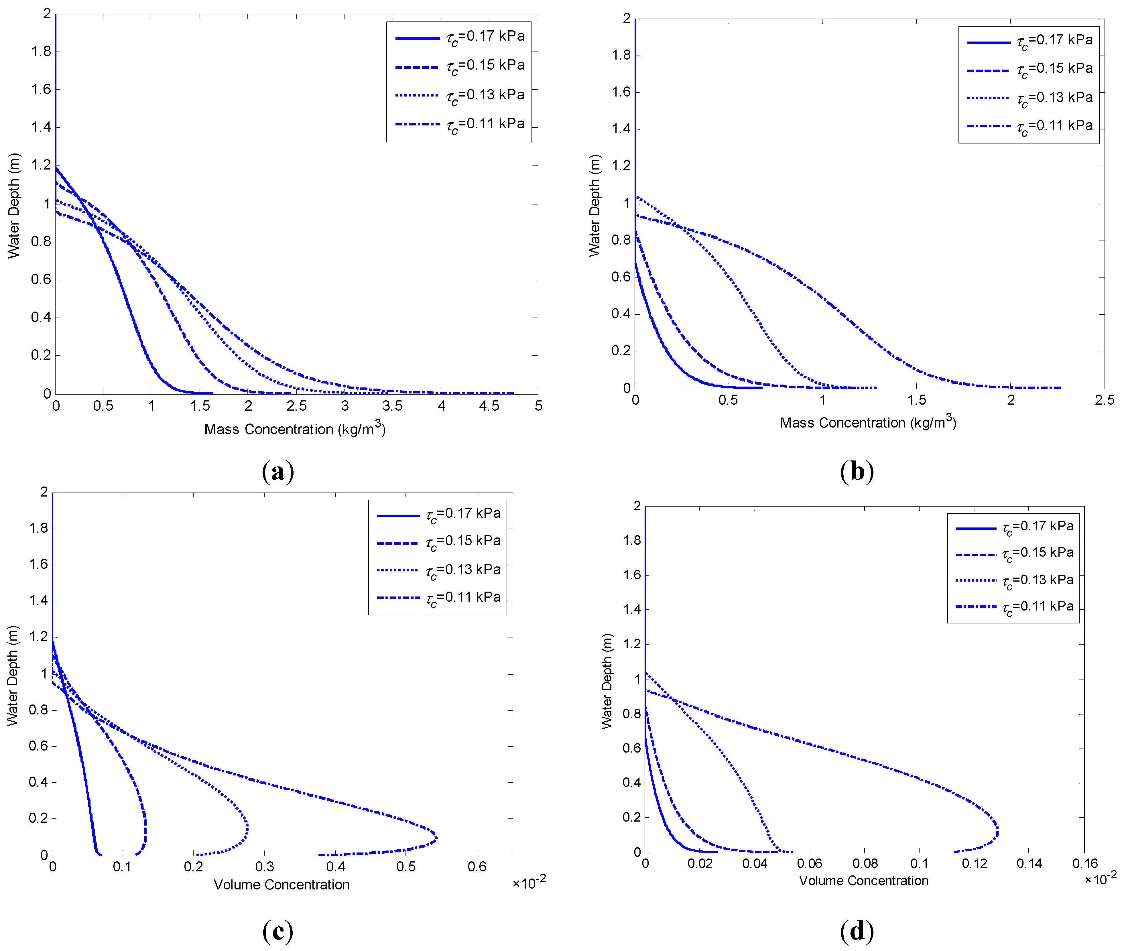
To examine the effect of mass concentration on volumetric concentration, concentration profiles calculated with different values of τ_c are plotted in Figure 4. The solid, dashed, dotted, and dash-dotted curves represent calculation results under the conditions of τ_c = 0.17 kPa, τ_c = 0.15 kPa, τ_c = 0.13 kPa, and τ_c = 0.11 kPa, respectively. When u_avg is set to be 0.4 m/s, the elevated maximum of volumetric concentration is calculated as τ_c is decreased from 0.17 to 0.15 kPa. In the case of u_avg = 0.35 m/s, the elevated maximum is calculated with τ_c = 0.11 kPa. As shown in Figure 4a,b, the mass concentration is increased according to decrease of τ_c. The increased mass concentration enhances the aggregation process (the first term of Equation (1)) resulting in calculating the elevated maximum of volumetric concentration.

Figure 4. Vertical profiles of concentrations under different conditions of critical shear stress. (a) The mass concentration under the condition of u_avg = 0.40 m/s; (b) The mass concentration under the condition of u_avg = 0.35 m/s; (c) The volumetric concentration under the condition of u_avg = 0.40 m/s; (d) The volumetric concentration under the condition of u_avg = 0.35 m/s. The solid, dashed, dotted, and dash-dotted curves represent results of τ_c = 0.17 kPa, τ_c = 0.15 kPa, τ_c = 0.13 kPa, and τ_c = 0.11 kPa, respectively.

Figure 4. Vertical profiles of concentrations under different conditions of critical shear stress. (a) The mass concentration under the condition of u_avg = 0.40 m/s; (b) The mass concentration under the condition of u_avg = 0.35 m/s; (c) The volumetric concentration under the condition of u_avg = 0.40 m/s; (d) The volumetric concentration under the condition of u_avg = 0.35 m/s. The solid, dashed, dotted, and dash-dotted curves represent results of τ_c = 0.17 kPa, τ_c = 0.15 kPa, τ_c = 0.13 kPa, and τ_c = 0.11 kPa, respectively.

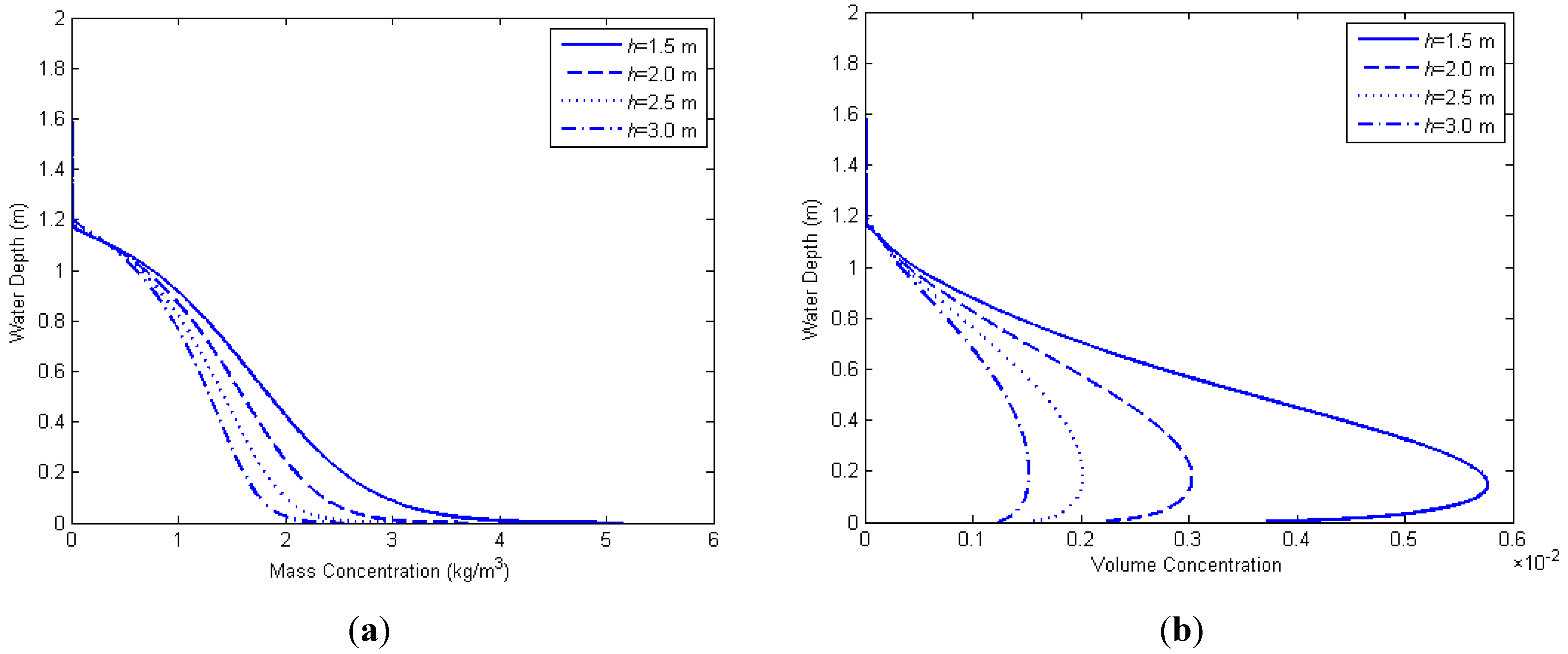
To investigate the effect of water depth (h) on the profile of volumetric concentration, different conditions of h are tested (Figure 5). In all cases of h, u_avg and τ_c are set to be 0.45 m/s and 0.17 kPa. As shown in Figure 5a, the mass concentration is increased in accordance with decrease of h whereas the suspension height is almost constant. Figure 5b represents the profiles of volumetric concentration. In Figure 5b, it is found that the vertical gradient of the volumetric concentration and the elevated maximum become more significant as h decreases. The profiles of mass concentration and volumetric concentration under the condition of h = 3.0 m are similar to those of h = 2.0 m and τ_c = 0.15 kPa (see Figure 4a,b).

Figure 5. Vertical profiles of concentration under different conditions of water depth (h). (a) The mass concentration profiles; and (b) The volumetric concentration profiles. The solid, dashed, dotted, and dash-dotted curves represent results of h = 1.5 m, h = 2.0 m, h = 2.5 m, and h = 3.0 m, respectively.

Figure 5. Vertical profiles of concentration under different conditions of water depth (h). (a) The mass concentration profiles; and (b) The volumetric concentration profiles. The solid, dashed, dotted, and dash-dotted curves represent results of h = 1.5 m, h = 2.0 m, h = 2.5 m, and h = 3.0 m, respectively.

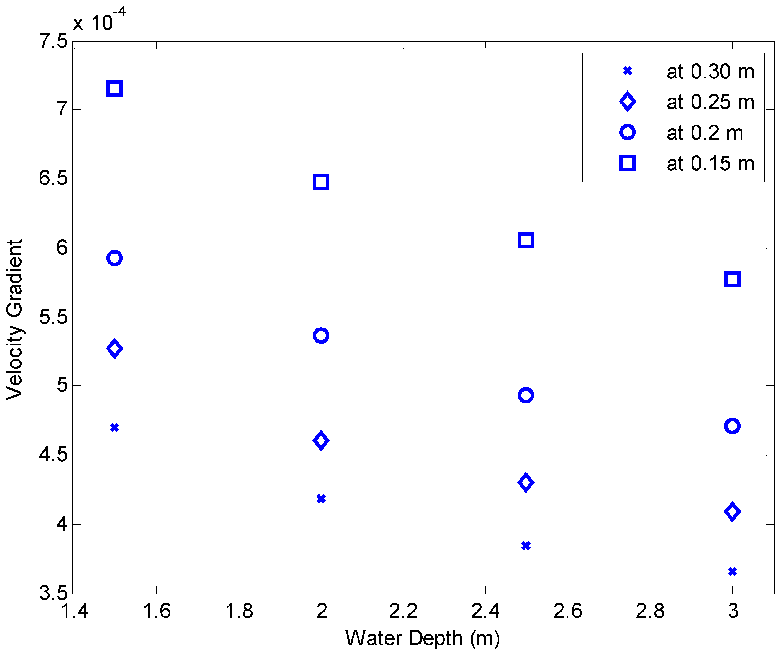
From this finding, it is known again that the shape of volumetric concentration significantly depends on mass concentration. Figure 6 shows the gradient of u_avg at the elevations of 0.30 m, 0.25 m, 0.20 m, and 0.15 m under the condition of Figure 5. It is found in Figure 6 that the velocity gradient near the bed decreases as the water depth increases. The fluid shear stress is considered to be proportional to the velocity gradient under the assumption of Newtonian shear stress relationship. Based on Newtonian shear stress relationship, it can be seen in Figure 6 that the fluid shear is also decreased as the water depth increases. Therefore, the sediment suspension is affected by the water depth under the constant conditions of u_avg and τ_c. However, the water depth is not considered as a dominant factor to determine the occurrence of elevated maximum because the elevated maximum of volumetric concentration is found in all cases of elevations tested in this study. This is also found in the study of Fox et al. [31]. In Figure 4 of Fox et al. [31], the elevated maximum of volumetric concentration is found at many different elevations. However, it is also difficult to make a generalized conclusion with Fox et al. [31] because of the hydrodynamics changes at different locations of measurement. In addition, it is impossible to replicate the measurements of Fox et al. [31] using a numerical model due to limited information on the hydrodynamic conditions of the measurements.

From Equation (4), it is known that ${\mathrm{\varphi }}_f$ is inversely proportional to the solid volume concentration of the primary particles within a floc, ${\mathrm{\varphi }}_{sf}$, defined below:

$${\mathrm{\varphi }}_{sf}=\frac{{\mathrm{\rho }}_f-{\mathrm{\rho }}_w}{{\mathrm{\rho }}_s-{\mathrm{\rho }}_w}=\frac{V_s}{V_f}$$

(18)

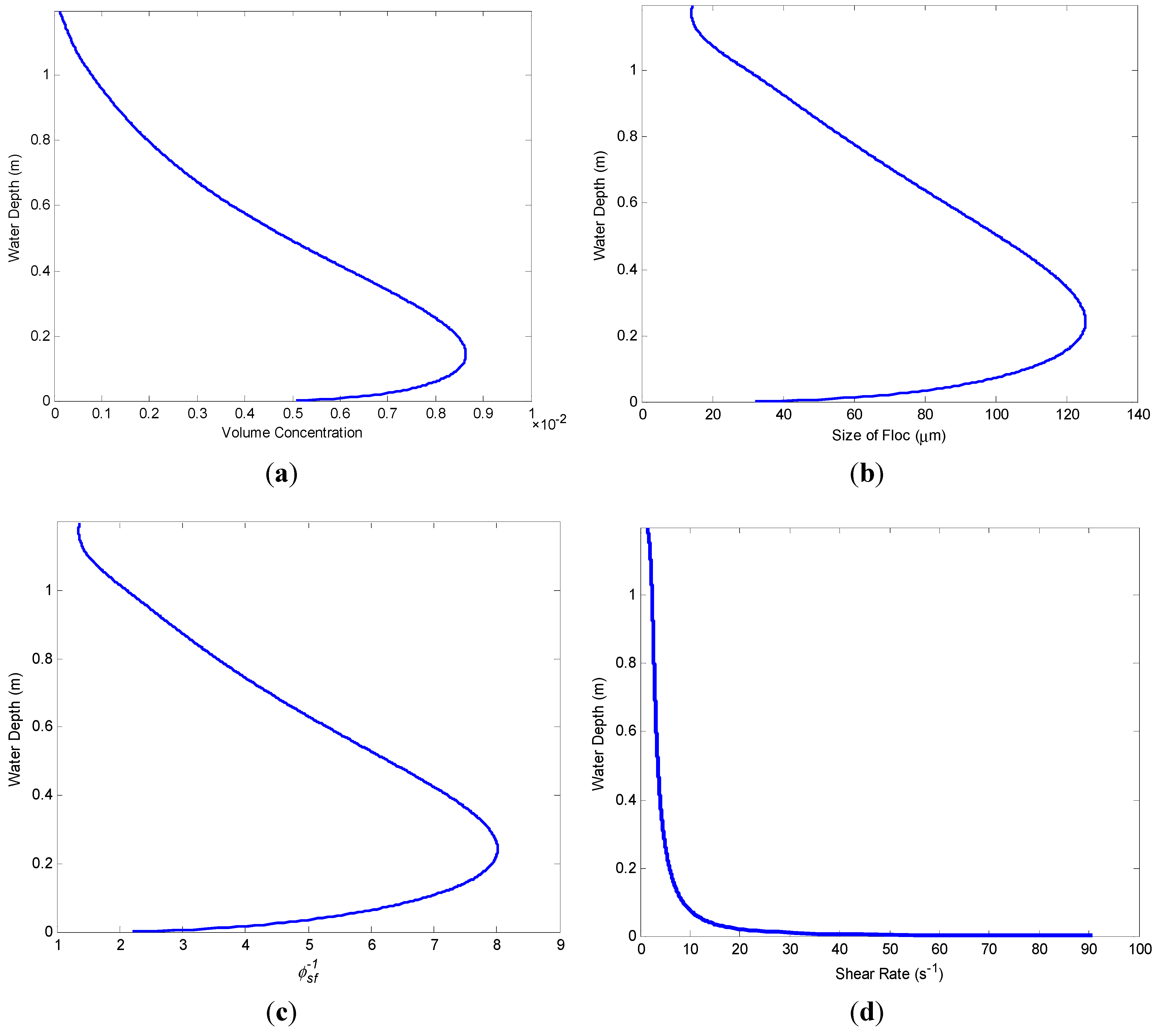
where V_f = volume of a floc; V_s = volume of primary particles within a floc; and ${\mathrm{\varphi }}_{sf}$ = ratio of the total volume of solids in a floc to the volume of a floc. Figure 7 shows the vertical profiles of ${\mathrm{\varphi }}_{sf}^{-1}$, ${\mathrm{\varphi }}_f$, D, and G when the elevated maximum of ${\mathrm{\varphi }}_f$ occurs. It is found in Figure 7 that ${\mathrm{\varphi }}_{sf}^{-1}$ and D have the same shape and elevation of maximum values. The elevation of maximum ${\mathrm{\varphi }}_{sf}^{-1}$ and D is slightly higher than that of ${\mathrm{\varphi }}_f$. The elevated maximum of ${\mathrm{\varphi }}_f$ means that larger flocs of which ${\mathrm{\varphi }}_{sf}$ is low exist near the location of the concentration maximum (see Figure 7a,b). From the low values of ${\mathrm{\varphi }}_{sf}^{-1}$ and D near the bed, it is also known that small and dense flocs, which have a large yield stress (see [38]), exist near the bed. A floc has a high density and a small size when the turbulence intensity is strong. Therefore, the intensity of turbulence near the elevation of the maximum value of ${\mathrm{\varphi }}_f$ is expected to be low whereas the turbulence intensity near the bed has a high value. Figure 7d shows the profile of G, which is a measure of turbulence intensity. G near the bed is about 90 s⁻¹ whereas G near the elevation of the maximum value of ${\mathrm{\varphi }}_f$ is about 5 s⁻¹. The strong turbulence near the bed enhances the breakup process of flow resulting in a small and dense floc. The low intensity of turbulence near the elevation of maximum ${\mathrm{\varphi }}_f$ causes growth of flocs having a low density and a large size. Mikkelsen et al. [46] measure the volumetric concentration at four different locations by estimating a proxy for current stress based on the squared current velocity. It is found in Mikkelsen et al. [46] that the volumetric concentration increases at the location where the current stress is high. It is also concluded in Mikkelsen et al. [46] find that the strong turbulence causes the erosion of micro-flocs (not primary particles) from the bed. This conclusion is consistent with the findings of this study. The floc size is calculated to be small near the bed due to the high intensity of turbulence (see Figure 7).

Figure 6. Variation of velocity gradients under different conditions of water depth. The asterisk, diamond, circle, and square symbols represent results at elevations of 0.3 m, 0.25 m, 0.2 m, and 0.15 m, respectively. The experimental condition is consistent with Figure 5.

Figure 6. Variation of velocity gradients under different conditions of water depth. The asterisk, diamond, circle, and square symbols represent results at elevations of 0.3 m, 0.25 m, 0.2 m, and 0.15 m, respectively. The experimental condition is consistent with Figure 5.

Figure 7. Vertical profiles of ϕ_f, D, ${\mathrm{\varphi }}_{sf}^{-1}$, and G. In Figure 7c, the inverse of ϕ_sf is plotted for convenience. (a) Volumetric concentration; (b) Floc size; (c) Solid volume concentration within a floc; and (d) Shear rate.

Figure 7. Vertical profiles of ϕ_f, D, ${\mathrm{\varphi }}_{sf}^{-1}$, and G. In Figure 7c, the inverse of ϕ_sf is plotted for convenience. (a) Volumetric concentration; (b) Floc size; (c) Solid volume concentration within a floc; and (d) Shear rate.

4. Conclusions

This study aims to investigate the characteristics of cohesive sediment suspension, with Specific focus on the elevated maximum of volumetric concentration is intensively discussed here. The decrease of volumetric concentration near the bed is found when the flocculation process is active (i.e., the mass concentration is high enough). The strong turbulence, which is quantified by G in this study, near the bed enhances the breakup process resulting in a decrease of floc size and an increase of floc density. In this region, the floc size is kept to be relatively small. Therefore, small and dense flocs exist near the bed. This idea is consistent with studies of Spicer et al. [22] and Mikkelsen and Pejrup [6]. Spicer et al. [22] and Mikkelsen and Pejrup [6] insist that the floc breakup occurs at the weakest part of the floc structure. This produces smaller fragments density and yield stress of which are higher than those of the parent floc. Dyer [7] argues that particle collisions become more significant as the mass concentration increases. Based on Dyer [7], it is deduced that the volumetric concentration decreases near the bed where the turbulence intensity is strong and the mass concentration is high. The increase of turbulence intensity near the bed is explained in many studies (e.g., [33,47]). The density of floc depends on the fractal dimension. From the study of Khelifa and Hill [11], it is known that the density of floc has a inversely proportional relationship with floc size because the fractal dimension decreases as the size of floc increases. Therefore, the decreased size and increased density of flocs can cause the lower volumetric concentration even if the mass concentration increases.

It is obvious that flocs experience a sufficient size increase at an elevation where G is low. For the suspension of particles up to this elevation, a high erosion flux from the bed is needed. The erosion flux is determined by the difference between the critical shear stress and the bottom fluid stress. Therefore, the elevated maximum is also affected by the critical shear stress under the condition of constant flow velocity.

This study also shows that the elevated maximum has a close relationship with the flocculation process rather than with flow type and water depth. Dey et al. [33] conducted experiments using non-cohesive sediment. Considering the effect of suspended sediment on turbulence, it is questionable wether the results of cohesive sediment are consistent with the study of Dey et al. [33]. Therefore, in the future, it is necessary to carry out well-controlled laboratory experiments using cohesive sediment.