Article

Potential Impacts of Climate Change on Precipitation over Lake Victoria, East Africa, in the 21st Century

1
Department of Civil Engineering, KU Leuven, Kasteelpark Arenberg 40, bus 2448, Leuven 3001, Belgium
2
Department of Civil and Environmental Engineering, Makerere University Kampala, P. O. Box 7062, Kampala 00256, Uganda
3
Department of Hydrology and Hydraulic Engineering, Vrije Universiteit Brussel, Pleinlaan 2, Brussels 1050, Belgium
*
Authors to whom correspondence should be addressed.
Water 2014, 6(9), 2634-2659; https://doi.org/10.3390/w6092634
Submission received: 3 June 2014 / Revised: 21 August 2014 / Accepted: 22 August 2014 / Published: 29 August 2014
(This article belongs to the Special Issue Water Resources in a Variable and Changing Climate)

Abstract

:
Precipitation over Lake Victoria in East Africa greatly influences its water balance. Over 30 million people rely on Lake Victoria for food, potable water, hydropower and transport. Projecting precipitation changes over the lake is vital in dealing with climate change impacts. The past and future precipitation over the lake were assessed using 42 model runs obtained from 26 General Circulation Models (GCMs) of the newest generation in the Coupled Model Intercomparison Project (CMIP5). Two CMIP5 scenarios defined by Representative Concentration Pathways (RCP), namely RCP4.5 and RCP8.5, were used to explore climate change impacts. The daily precipitation over Lake Victoria for the period 1962–2002 was compared with future projections for the 2040s and 2075s. The ability of GCMs to project daily, monthly and annual precipitation over the lake was evaluated based on the mean error, root mean square error and the frequency of occurrence of extreme precipitation. Higher resolution models (grid size <1.5°) simulated monthly variations better than low resolution models (grid size >2.5°). The total annual precipitation is expected to increase by less than 10% for the RCP4.5 scenario and less than 20% for the RCP8.5 scenario over the 21st century, despite the higher (up to 40%) increase in extreme daily intensities.

1. Introduction

Lake Victoria, Africa’s largest fresh water lake covers a surface area of about 68,800 km2 shared across three East African countries: Uganda (45%), Kenya (6%), and Tanzania (49%). Over 30 million inhabitants depend on Lake Victoria for their livelihoods. Therefore, precipitation changes over the lake are likely to affect the quality of life of many within the East Africa region. Lake Victoria has a complex shoreline structure comprising gulfs and bays that provide potable water abstraction points and also receive municipal and industrial waste from adjacent urban centers.
Due to the vast size of the Lake Victoria basin, it is considered that the average annual lake precipitation almost balances the annual evapotranspiration. Therefore, precipitation variations significantly influence water levels in Lake Victoria. This notion has been applied by several authors to study the water balance of the lake, often translated as changes in the lake levels or outflow regimes—with most variations in the water balance being attributed to the different calculation periods and methods used in estimation of the different balance components i.e., evapotranspiration, inflows, outflows and precipitation [1,2,3,4,5]. About 80% of the Lake Victoria refill is predominantly precipitation compared to the 20% from basin discharge [6]. Satellite remote sensing data was applied in [7] to monitor the water balance of Lake Victoria in comparison to other water bodies in the vicinity—climate forcing explained half of the lake level trends while the outflow patterns were responsible for the other half. Climate forcing is generally affected by the amount of aerosols and greenhouse gases (GHG) in the atmosphere. GHGs absorb and re-emit energy radiated from the Earth's surface, leading to a warming or cooling effect and changes in the Earth’s energy balance with time. Increasing greenhouse gas concentrations in the atmosphere leads to warming which in turn causes global atmospheric water vapor and precipitation to increase. Aerosols directly absorb and scatter incoming solar radiation leading to cooling at the surface and a reduction in precipitation. They can also affect precipitation through complex interactions with clouds [8]. At regional scales, changes in precipitation can also be influenced by anthropogenic activities that affect atmospheric transport of water vapor and circulation changes.
The importance of global precipitation changes as addresssed in [8] by the Intergovernmental Panel on climate Change (IPCC) fifth Assessment Report (AR5) suggests a need to understand and project effects of extreme climate conditions. This paper evaluates the newest generation models used in the CMIP5 project with the purpose of studying impact of climate change on the quantity and quality of water in Lake Victoria. Precipitation was aggregated at different temporal scales; daily, monthly and annually. Model evaluation was based on a range of statistical measures and visual graphical comparison for the same aggregation periods in order to postulate possible precipitation changes over Lake Victoria.

2. Data and Methods

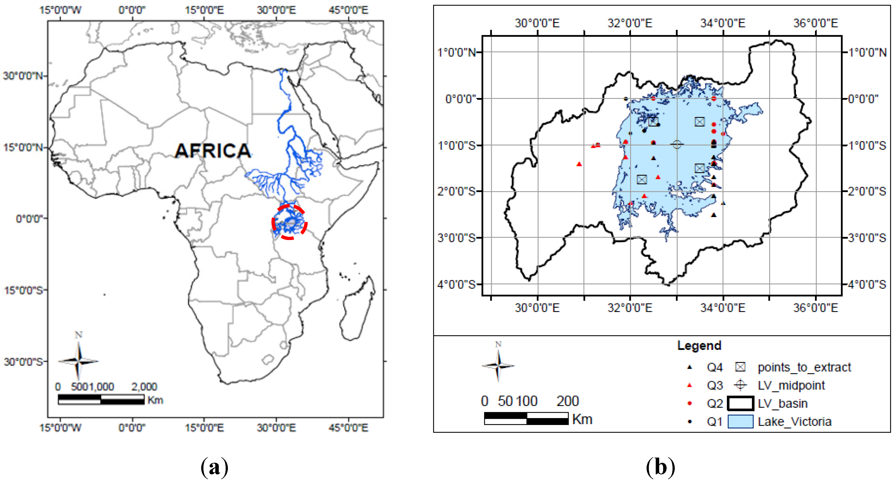
2.1. Description of the Study Area

Lake Victoria is located in the upper Nile basin in East Africa within latitudes 00°30′00″ N to 03°00′00″ S and longitudes 31°30′00″ E to 35°00′00″ E. The Lake surface is at an average elevation of about 1135 m.a.s.l (Figure 1). Lake Victoria covers a total catchment area of about 258,000 km2. The lake itself contributes about 27% of the total catchment area. Generally, the Lake Victoria basin climate is characterized by substantial precipitation occurring throughout the year; however, there are two distinct rainy seasons in which monthly precipitation is generally greater than 10% of the average monthly precipitation. Heavier precipitation occurs in the March-April-May (MAM) season, while the longer rainy season occurs in October-November-December (OND). Climate variability for the lake basin region is influenced by both large-scale and meso-scale circulations resulting from complex interactions of the Inter-Tropical Convergence Zone (ITCZ) and El Nino Southern Oscillation (ENSO), Quasi-biennial Oscillations, large-scale monsoonal winds, and extra-tropical weather systems [9,10,11,12].
Figure 1. (a) Location of Lake Victoria within Africa; (b) Coordinates where general circulation model (GCM) precipitation output for Lake Victoria was extracted.
Water 06 02634 g001

2.2. Precipitation and Lake Levels

Precipitation over Lake Victoria experienced a predominantly positive trend over the 20th century [12]. A sharp increase in water levels occurred in 1962—it was mainly attributed to the high precipitation in that year and the related high tributary inflows [3,13]. Precipitation occurrence had the largest effect on the lake levels and flow exiting the basin at the Victoria Nile river, while irrigation and hydropower developments had modest effects on these levels and flows [14]. However, commissioning of the Owen Falls Dam, located on the White Nile in 1954 (just prior to the lake rise in 1962) could also have had an impact on the water levels as the lake regained its level as noted by [13,15]. Figure 2 shows the cumulative precipitation and discharge trends from the Lake Victoria catchments compared to the water levels in the lake. It can be deduced that tributary inflows were more significant in increasing lake levels in 1962 and 1998, which years coincided with the El Nino years [9,10] as depicted by the jumps in the cumulative tributary inflows. In conclusion, both human management roles and natural factors affected the lake levels, but precipitation clearly is the major factor. Climate change impact investigations on the Lake Victoria water levels therefore should focus on the future changes in precipitation.
Figure 2. Lake level variations over time compared to cumulative average precipitation over the lake and cumulative total inflow into the lake. The calculated lake level variations are based on the precipitation and inflow [16].
Water 06 02634 g002

2.3. Climate Model Simulations

General circulation models (GCMs) are numerical models that describe physical processes of the global climate system in the atmosphere, ocean, cryosphere and land surface in response to changing GHG and aerosol concentrations. GCMs provide geographical and physical estimates of regional climate and climate change using three dimensional grids over the globe. The newest generation GCMs are used in the CMIP5 to understand the past and future climate changes. These are the models upon which the recent Fifth Assessment Report (AR5) of the IPCC is based [8]. The CMIPs attempt to address major priorities and incorporate ideas from a wide range of climate modelling communities. The climate change modelling experiments are integrated using atmosphere-ocean global climate models (AOGCMs). These models respond to specified, time-varying concentrations of various atmospheric constituents e.g., GHGs and include interactive representation of the atmosphere, ocean, land and sea ice. CMIP5 also introduces coupling of biogeochemical components to account for closing of carbon fluxes between the oceans, atmosphere and terrestrial biosphere carbon reservoirs for long term simulations in the earth system models. They are capable of using time-evolving emissions of constituents to interactively compute concentrations.
The main difference between these CMIP5 projections and the previous CMIP projections is that their climate change projections include policy intervention and mitigation measures [17]. CMIP5 provides a large set of runs that enable systematic model inter-comparison within each type of experiment and credible multi-model analysis. The core experiments include the historical runs covering much of the industrial period (mid-19th century to the near-present) and future projection simulations forced with specific GHG concentrations and anthropogenic aerosols emissions dubbed “Representative Concentration Pathways” (RCPs) e.g., RCP4.5 and RCP8.5. RCP8.5 is consistent with the high emissions scenario in which the radiative forcing increases throughout the 21st century before reaching 8.5 Wm−2 at the end of the century, while RCP4.5 signifies a mid-range mitigations emissions scenario where GHG valuation policies are applied to stabilize atmospheric radiative forcing to 4.5 Wm−2 in 2100 (Figure 3). These two CMIP5 scenarios were considered in this study as a basis of exploring climate change impacts and policy issues. RCPs enable investigations of uncertainties related to carbon cycle and atmospheric chemistry. They span a wide range of total forcing values though they do not cover the full range of emissions in the literature, particularly for aerosols [8].
Figure 3. Representative concentration pathways. (a) Changes in radiative forcing relative to pre-industrial conditions; (b) Energy and industry CO2 emissions for the different representative concentration pathway (RCP) candidates. The range of emissions in the recent (post 2001) literature is presented as a thick dashed curve for the maximum and minimum while the shaded area represents the 10th to 90th percentiles [17].
Water 06 02634 g003
According to [17], a realistic climate model should exhibit internal variability with spatial and temporal structure like the observed. However, in the long-term simulations, timing of individual unforced climate events like El Nino years in the historical runs will rarely (and only by chance) coincide with years of actual occurrence, since historical runs are initiated from an arbitrary point of quasi-equilibrium control run. Hence, the results should be analyzed in probabilistic terms in a similar manner as [18,19,20].
GCMs that were used for both RCP8.5 and RCP4.5 simulations were applied to project the precipitation patterns over Lake Victoria for the 2040s (2020–2060) and 2075s (2055–2095). The historical and future precipitation for the 2040s and 2075s was obtained by simply averaging the simulations from the different GCMs. This method is opposed to applying weighting factors described in [21] and was applied to avoid introducing extra uncertainties as tested by [22]. A total of 42 GCM runs obtained from 26 models simulated by 16 different modeling centers of the CMIP5 archive were used. GCM simulations for the historical period were obtained for the different quarters of Lake Victoria (Figure 1) and averaged to obtain the areal precipitation over the lake.
The performance of GCMs was evaluated based on the historical outputs using the absolute observed precipitation series over the lake for the 41-year period 1962–2002 provided by [12]. Precipitation measurements over the lake are sparse and of low quality. Kizza [16] compared satellite measurements to the lake surrounding observations—TRMM 3B43 product improved the quality of precipitation over the lake by 33% while the PERSIANN product improved the precipitation series by 76%. Kizza et al. [12] improved the spatial precipitation input using gridded monthly precipitation with a spatial resolution of 2 km for both ground based and satellite data for the period 1960–2004 providing a plausible lake balance model (Figure 2).
Due to the variation in GCM outputs and for clearer analysis of results, the precipitation simulations by the GCMs were further classified according to the GCM grid sizes. The spatial resolution of the CMIP5 coupled models range from 0.5° to 4° for the atmospheric component and 0.2° to 2° for the ocean component [17]. Table 1 shows an overview of the 26 GCMs used in this study. The model resolutions are classified as follows: Low Resolution (LR) models: grid size >2°, Medium Resolution (MR) models: 1.5° to 2°, High Resolution (HR) models: <1.5° based on their seasonal performance.
Table 1. Coupled Model Intercomparison Project (CMIP5) general circulation models (GCMs) considered in this study; blue (b), green (g) and red (r).
Modeling CenterCountryModelLat.Lon.Res.Color
i.  Commonwealth Scientific and Industrial Research Organization/ Bureau of Meteorology (CSIRO-BOM)AustraliaACCESS1.01.871.25MRg
ii.  College of Global Change and Earth System Science, Beijing Normal UniversityChinaBNU-ESM2.812.79LRr
iii.  Centro Euro-Mediterraneo per I Cambiamenti ClimaticiItalyCMCC-CESM3.753.71LRr
ItalyCMCC-CMS1.871.87MRg
iv.  Centre National de Recherches Meteorologiques / Centre Europeen de Recherche et Formation Avancees en Calcul Scientifique (CNRM/CERFACS)FranceCNRM-CM51.411.40HRb
v.  Commonwealth Scientific and Industrial Research Organization/ Queensland Climate Change Centre of Excellence (CSIRO-QCCCE)AustraliaCSIRO-Mk3.61.871.87MRg
vi.  Canadian Centre for Climate Modelling and AnalysisCanadaCanESM22.812.79LRr
vii.  Geophysical Fluid Dynamics LaboratoryUS-NJGFDL-ESM2G2.52.0LRr
US-NJGFDL-ESM2M2.52.0LRr
viii.  NASA Goddard Institute for Space StudiesUS-NYGISS-E2-H2.52.0LRr
US-NYGISS-E2-R2.52.0LRr
ix.  Met Office Hadley CentreUK-ExeterHadCM33.752.5LRr
UK-ExeterHadGEM2-CC1.871.25MRg
UK-ExeterHadGEM2-ES1.751.25MRg
x.  Institut Pierre-Simon LaplaceFranceIPSL-CM5A-LR3.751.89LRr
FranceIPSL-CM5A-MR2.501.26LRr
FranceIPSL-CM5B-LR3.751.89LRr
xi.  Atmosphere and Ocean Research Institute (The University of Tokyo), National Institute for Environmental Studies, and Japan Agency for Marine-Earth Science and TechnologyJapanMIROC-ESM2.812.79LRr
JapanMIROC51.401.40HRb
xii.  Max Planck Institute for Meteorology (MPI-M)GermanyMPI-ESM-LR1.871.87MRg
GermanyMPI-ESM-MR1.871.87MRg
xiii.  Meteorological Research InstituteJapanMRI-CGCM31.121.12HRb
xiv.  Norwegian Climate Centre (NCC)NorwayNorESM1-M2.501.89LRr
xv.  Beijing Climate Center, China Meteorological AdministrationChinaBCC-CSM1.1m1.121.12HRb
ChinaBCC-CSM1.12.812.79LRr
xvi.  Institute for Numerical MathematicsRussiaINM-CM42.01.5MRg

2.4. Model Performance Evaluation

Probabilistic analyses were performed to evaluate the effect of climate change on absolute precipitation for different aggregation scales i.e., yearly, monthly, daily; and to investigate reasons for the precipitation changes. The GCM performance was analyzed for the different seasons i.e., January-February (JF), March-May (MAM), June-September (JJAS) and October-December (OND) based on the Normalized Mean Error (NME) and the covariance between the observed and historical GCM output. The NME is defined as the ratio of mean error to sample mean of the observations, while covariance is a measure of how two variables change together—positive covariance implies variables increase or decrease together. Evaluation of GCM performance for annual precipitation was based on the Coefficient of Variation of the Root Mean Square Error (CV(RMSE)) as well. The CV(RMSE) was computed as the ratio of the RMSE to the mean of the observations. The ability of the GCMs to simulate high and extreme precipitation was checked for daily, monthly and annual time scales. For that purpose, precipitation amounts were ranked and plotted against the empirical return period to determine how well the GCMs perform in extreme precipitation distributions. This analysis is useful from a water engineering point of view: If the GCM results would be used for obtaining water engineering design or planning values in terms of precipitation amount for given return periods, the analysis shows the deviations that can be found in these design or planning values.
One important remark should be made about this GCM performance evaluation based on historical precipitation observations: model performance for the historical period, as evaluated here, is not equivalent to future model performance. The latter obviously cannot be validated; that is why the historical analysis is used instead as indicative for future performance.
To determine the influence of future climate change on precipitation, the ratios of potential future simulated precipitation to historical precipitation simulations—hereafter referred to as perturbation factors, were used to project impacts of climate change in the Lake Victoria basin. This approach has been applied to study climate change by several authors e.g., [19,23]. The source of future changes in precipitation reflected in the perturbation factors was further analyzed in the different seasons to understand the influence of individual effects like changes in intensities or number of wet days in each season on the global annual change using Box plots. This analysis aims to provide plausible quantifiable measures of precipitation changes over Lake Victoria in the 21st century.

3. Results and Discussion

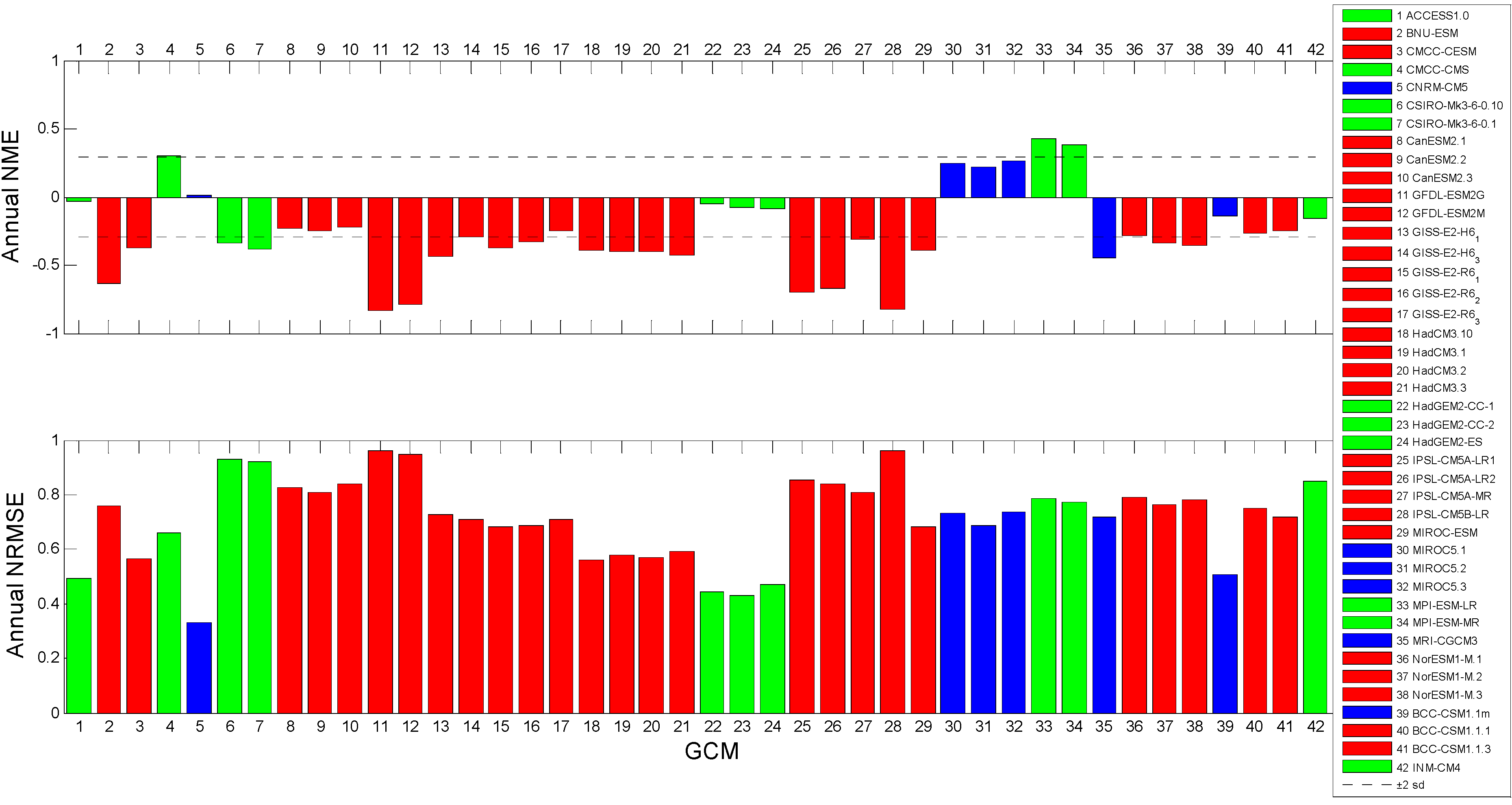
3.1. GCM Performance Evaluation

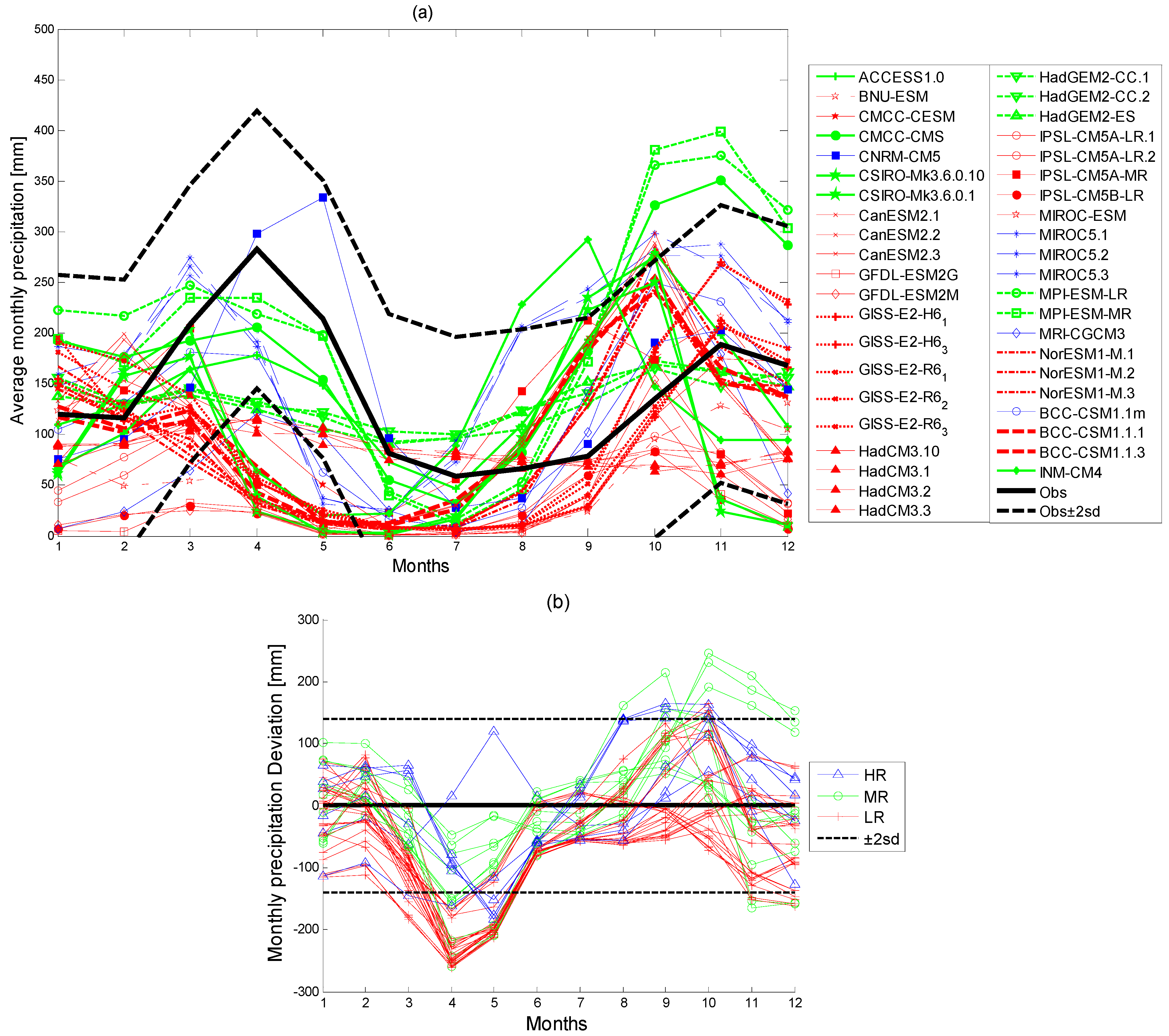
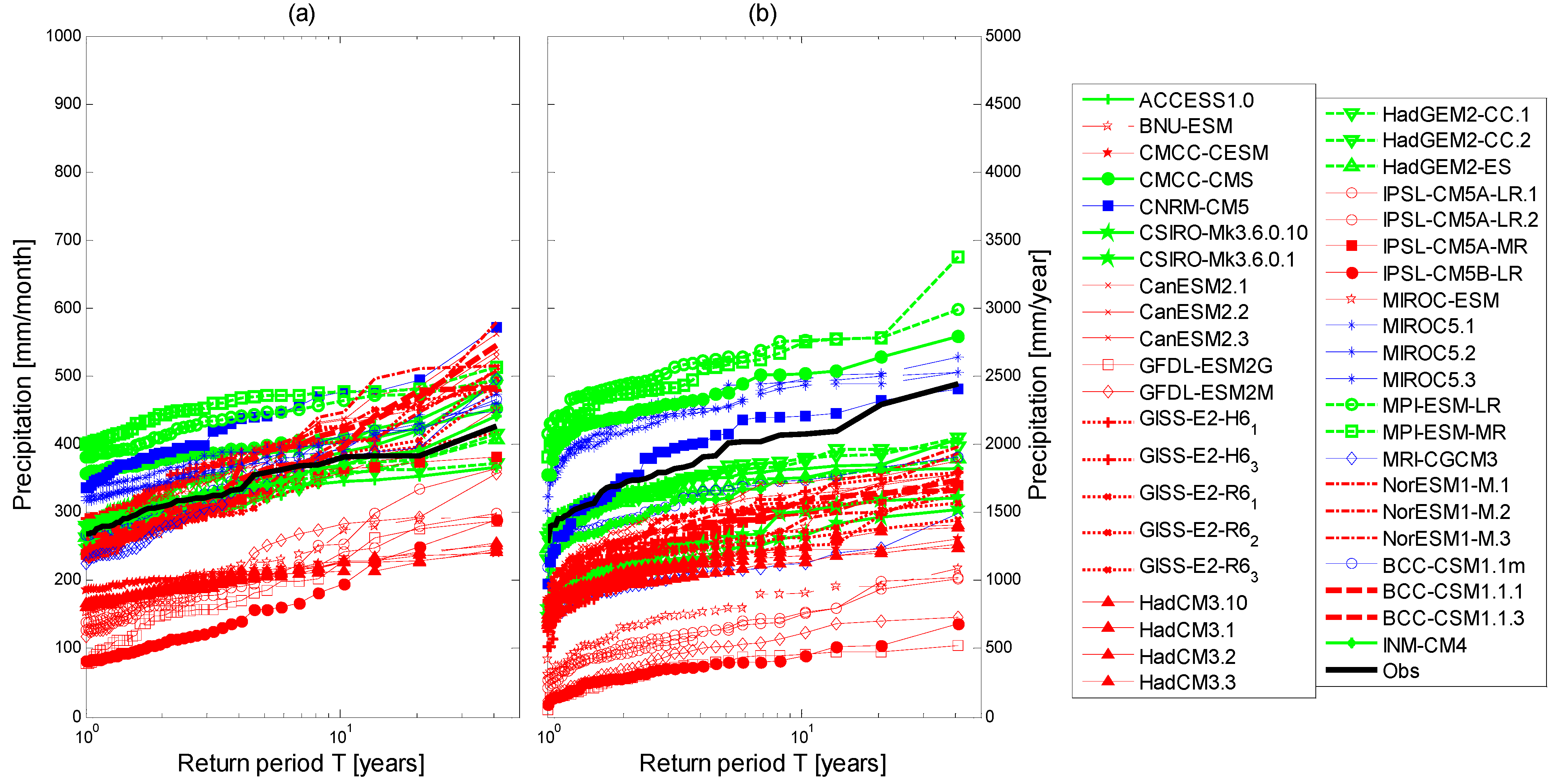
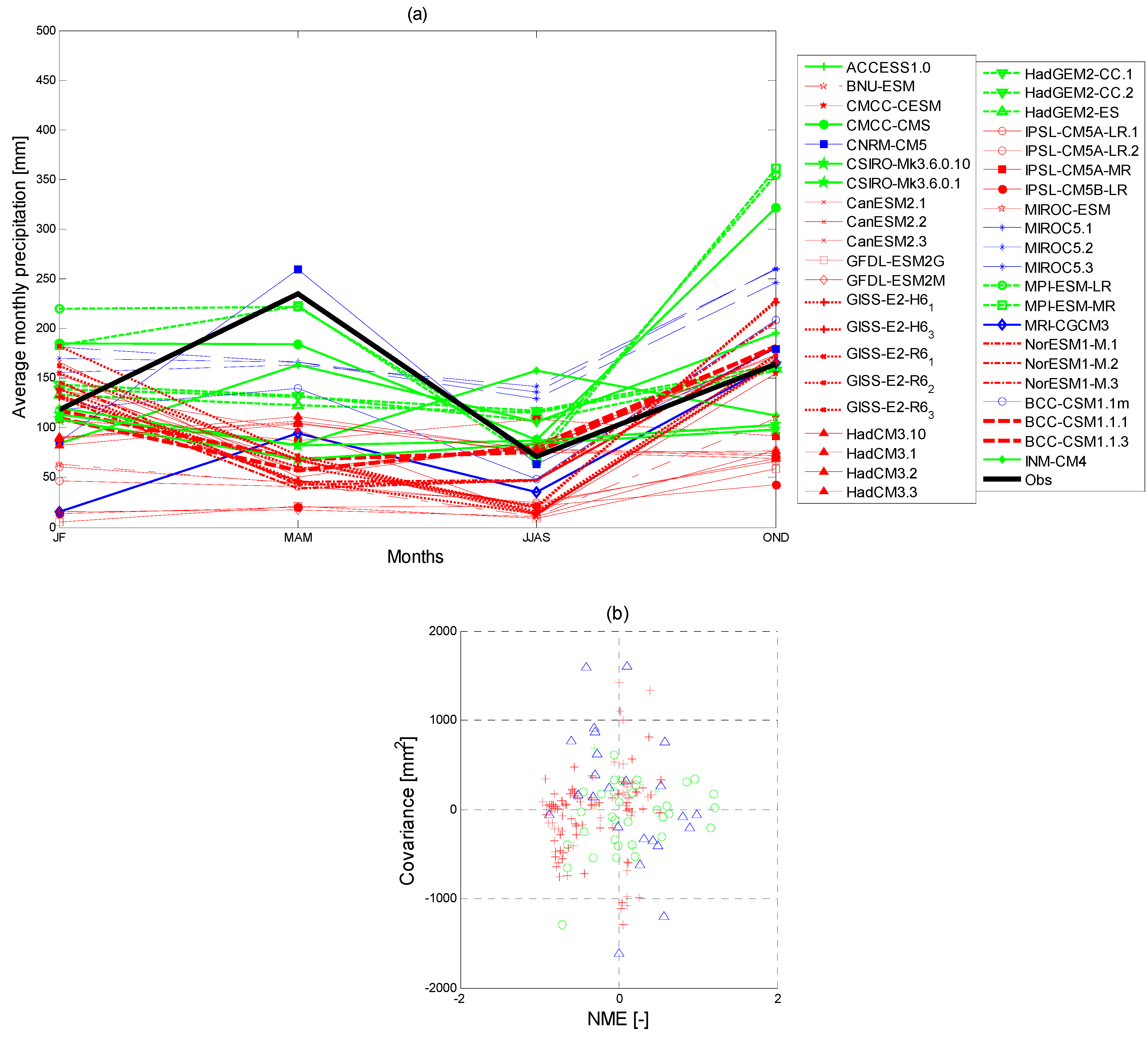
3.1.1. Monthly, Seasonal and Annual Precipitation

The GCM historical and observed series for the period 1962–2002 were aggregated over monthly time scales to evaluate the seasonal variations in the model based precipitation amounts and how much they deviate from the absolute observed values. This was done for the different resolution GCMs (Figure 4a). LR GCMs with grid sizes greater than 2° (>220 km) generally fail to simulate the wetter MAM rainy season depicted by the observed series while the HR GCMs (<165 km) show an acceptable seasonal pattern (Figure 4a). Based on the precipitation results only, the performance of the GCMs improved with the increase in resolution of the GCMs (Figure 4a). The different runs within the same GCMs did not necessarily produce a discrepancy as large as that between the different GCMs (Figure 4a) implying that model parameterization is probably more vital in determining GCM output compared to GCM initializations. For example, CanESM2.1, CanESM2.2, CanESM2.3 have different initializations but not different parameters compared to another model e.g., HadGEM2-CC.1 and HadGEM2-CC.2. From Figure 4a, we can see that differences between HadGEM-CC and CanESM2 models are larger than those arising between different runs within the same model.
Earlier research by [19] reported that there was no strong evidence to suggest that GCM performance improved with higher spatial resolution for the previous generation GCMs (4th Assessment Report of the IPCC based on CMIP3). Of the 18 GCMs of CMIP3 used by [19], only CCSM3.0 can be categorized as HR, based on the definition used in the present manuscript. The three other CMIP3 GCMs (MK3.0, MK3.5, and ECHAM5) similar to CSIRO-Mk3.6 and MPI-ESM-LR in CMIP5 are categorized as MR while the rest fall under LR models. HR and MR GCMs such as CCSM3.0, MK3.0, MK3.5 and ECHAM5 were ranked in the top five performing GCMs while most other GCMs performed poorly for the Katonga and Ruizi catchments, which are located within the Lake Victoria basin [19]. This study conforms to our hypothesis even though the areal extent of these catchments was in the order of 1000–3000 km2 [19] compared to the 68,800 km2 expanse of the lake. The improvement in the CMIP5 simulations in which higher spatial resolution coupled models were used to obtain a richer set of outputs cannot be neglected—however, IPCC [8] recognizes an undisputed similarity between CMIP3 and CMIP5 model simulations. This implies that model resolution was vital in determining the GCM performance.
Underestimation of monthly precipitation totals for the LR GCMs can be attributed to the large grid sizes that do not allow simulating different precipitation patterns over the northern and southern parts of the lake since rainfall patterns vary across the Lake Victoria basin. The universal kriging and inverse distance weighting methods used by [16] to obtain the spatial distribution of precipitation over the Lake Victoria basin show influence of the seasonal migration of the ITCZ on the rainy seasons such that the north eastern region generally receives more precipitation compared to the south eastern region. The GCMs underestimate precipitation in the rainy MAM season and the dry JJAS season, but overestimate the variable OND rainy season (Figure 4a,b). With the exception of the HadCM3 model, most GCMs simulate well the variable OND rainy season, which is highly influenced by complex interactions between the Indian and Pacific Oceans, a phenomenon that is well captured by the GCMs. HadCM3, HadGEM2-CC and HadGEM2-ES are developed by the same modeling center using similar radiative forcing. Although these models are essentially different, improved seasonal patterns are noticed in the finer HadGEM2-CC and HadGEM2-ES models compared to the coarser HadCM3 model (Figure 4a).
Figure 4. (a) Average monthly precipitation for the different GCMs compared to the observed series, red: Low resolution (LR) GCMs; blue: High resolution (HR) GCMs; green: Medium resolution (MR) GCMs; (b) Difference between modeled and observed precipitation for the different classifications of GCMs.
Water 06 02634 g004
There is a one month lag in the rainy seasons simulated by the GCMs as compared to the observed precipitation (Figure 4a). The monthly precipitation anomalies were calculated to account for the climatology simulated by the different GCMs as a difference between average monthly simulated precipitation, and the average monthly observed precipitation (Figure 4b). Most GCMs simulate the June-February precipitation well (lower monthly anomaly values) while the LR GCMs generally underestimate the MAM season even though there are more LR models compared to HR and MR models (Figure 4b). A more general seasonal check was applied in the JF, MAM, JJAS and OND seasons—to even out effects of the time lag exposed in Figure 4a, as shown in Figure 5a. The LR GCMs generally show lower (often negative) NME and covariance closer to zero or more negative implying that the observed and simulated historical seasonal precipitations did not change together for the LR models. From the covariance results (Figure 5b), it can be concluded that on average the tendency of a linear relationship between the observed and simulated seasonal precipitation decreased with increase in the grid size of the model. Most LR models showed negative covariance, while most HR models showed positive covariance for the average seasonal precipitation.
Figure 5. (a) Average seasonal precipitation for the different GCMs compared to the observed series for January-February (JF), March-May (MAM), June-September (JJAS) and October-December (OND) aggregations; (b) Covariance vs. normalized mean error (NME) for seasonal averages, red: LR GCMs; blue: HR GCMs; green: MR GCMs.
Water 06 02634 g005
Figure 6 shows the NME and its statistical significance compared to the uncertainty bounds approximated by twice the normalized standard deviation to approximate a 95% confidence interval. The best performing GCMs are again the higher resolution GCMs: CNRM-CM5, ACCESS1.0 and MRI-CGCM3, which lay within plotted uncertainty bounds. Figure 6 also shows the CV(RMSE) on the annual precipitation amounts. The GCMs: GFDL-ESM2G, GFDL-ESM2M, IPSL-CM5A-LR and IPSL-CM5B-LR (all of which are LR models) produce the highest CV(RMSE) and NME, henceforth are considered to be poorly performing. Generally, the GCMs perform better with the annual precipitation simulations compared to seasonal and monthly aggregations based on the NME (−1 to 2.5 for monthly; and −0.7 to 0.5 for annual aggregations in Figure 6).
Figure 6. NME and coefficient of variation of the root mean square error (CV(RMSE)) of average annual precipitation for the GCM simulations compared to the observed series, red: LR GCMs; blue: HR GCMs; green: MR GCMs.
Water 06 02634 g006
The GCMs show acceptable annual precipitation patterns (observed values located within the interval defined by the standard deviation of the GCM ensemble) but fail to simulate the peak precipitation (Figure 7a,b). The peak precipitation seasons are not well simulated in the GCMs; due to the inability of the GCMs to capture the heavy MAM precipitation even though model representation improves with increased model resolution. Although the peak annual precipitation is not well captured, the general annual variability trend is typically reproduced as it depends on the well simulated OND rainy season rather than the heavy MAM season. The OND and MAM seasons account for more than 65% of the total annual precipitation over the lake, however the variability of precipitation in the OND period has a greater influence on the annual precipitation compared to that in the MAM period [16]. The correlation coefficients between seasonal and annual precipitation totals for the OND and MAM periods were 0.71 and 0.5 respectively, i.e., peaks in annual precipitation totals tended to coincide with peaks in OND rather than MAM seasonal precipitation [24].
Figure 7. Annual variation of observed, and GCM output for (a) RCP4.5; (b) RCP8.5, GCM output bounds are based on twice the standard deviation.
Water 06 02634 g007

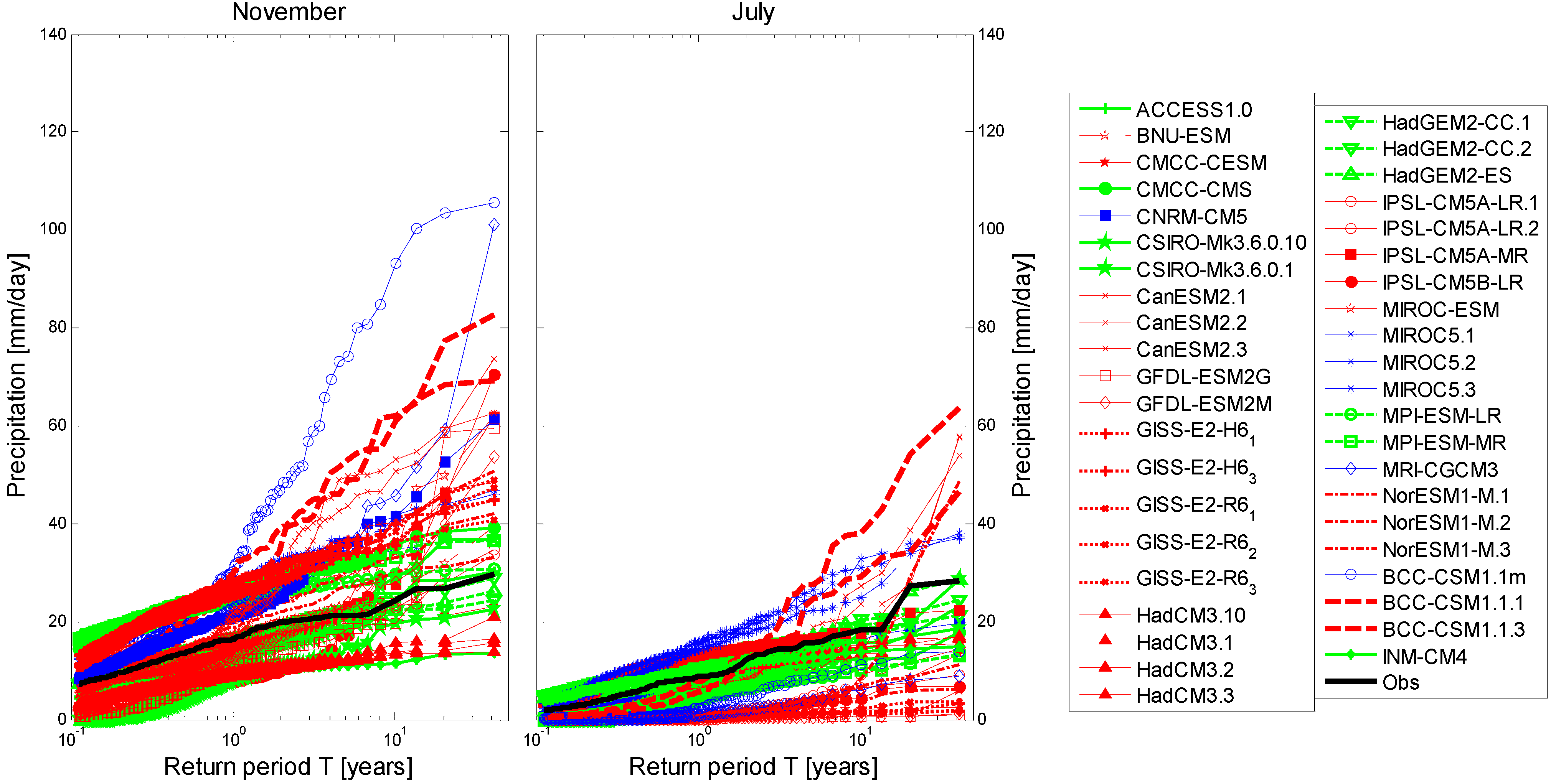
3.1.2. Precipitation Extremes

The LR GCMs underestimate the monthly and annual precipitation amount for given return periods (Figure 8). The underestimation of the precipitation amounts for the higher return periods is probably due to the large variations in topographical and areal properties that are evened out over wider areas while HR GCMs generally provide better simulations for monthly extremes. Some LR GCMs provide satisfactory monthly precipitation extremes, notably BCC-CSM1.1, IPSL-CM5A-MR, GISS-E2-H GISS-E2-R and NorESM-1 (Figure 8a)—this is misleading as monthly precipitation extremes are selected throughout the year yet the observed precipitation peaks in the MAM season may coincide with those in the OND season (Figure 4a). It is not surprising that the LR GCMs consistently simulated lower annual precipitation (Figure 8b). For this reason, monthly precipitation extremes are further classified in the different seasons in Section 3.1.2. CNRM-CM5 and MIROC5 gave the best estimations for both extreme monthly and annual precipitation as shown in Figure 8b.
The GCM performance was evaluated in the wet and dry months i.e., November and July respectively (Figure 9). For the rainy November, the uncertainty in simulating daily precipitation extremes with return periods higher than 4 years is very large, irrespective of the model resolution. The HR models overestimate the extreme precipitation amounts in the wet month of November. Many of these extreme events in the observed series are related to occurrence of El-Niño years as precipitation in the region is strongly quasi-periodic with a dominant ENSO timescale of variability of 5–6 years [9]. The monthly shift in the seasonal variations for the BCC-CSM1.1m, MRI-CGCM3 andBCC-CSM1.1 models was depicted in the daily extreme plots (Figure 9). These HR models overestimate extreme daily precipitation; yet in reality it is due to the one month time lag (Figure 4a). However, in July (the driest month), the GCM performance is very erratic with most LR GCMs underestimating the daily extremes. The uncertainty is higher in the driest month of July which experiences largely varying precipitation (Figure 9b).
Figure 8. (a) Return period of average monthly precipitation; (b) Average annual precipitation for the different GCM simulations as compared to the observed series; red: LR GCMs; blue: HR GCMs; green: MR GCMs.
Water 06 02634 g008
Figure 9. Return period of average daily precipitation for the different GCM simulations for November and July, red: LR GCMs; blue: HR GCMs; green: MR GCMs.
Water 06 02634 g009
The GCM evaluation showed that GCM outputs provide better results in terms of annual and seasonal precipitation compared to the daily scale analyses (Figure 8, Figure 9). Even if model performance cannot be evaluated based on a single index, an array of measures, such as those described in this section provide a good indication of the model overall performance. Higher resolution models provide better estimates of annual, seasonal and monthly precipitation; and precipitation variation (Figure 4, Figure 5, Figure 8). Table 2 provides a ranking of the good and poor performing GCMs based on annual, seasonal and monthly performance. Differences in latitudes are more significant in GCM precipitation performance than the differences in longitudes. CNRM-CM5 provides the best estimate for annual precipitation and seasonal variation with a minimum time shift in monthly simulations while HadCM3 fails to describe even the basic seasonal variation. As shown by Shaffrey et al. [25], reduction of the horizontal resolution e.g., in the HadGEM1 model, may result in reduced SST errors and more realistic approximations of small scale processes, especially the ENSO phenomenon leading to improvement of results simulated by the finer HiGEM model.
Table 2. Ranking of CMIP5 GCMs based on simulation of precipitation over Lake Victoria.
Good Performing GCMsLong.Lat.ResolutionPoor Performing GCMsLong.Lat.Resolution
CNRM-CM51.411.40HighHadCM33.752.5Low
MIROC51.401.40HighIPSL-CM5A-LR3.751.89Low
BCC-CSM1.1m1.121.12HighIPSL-CM5B-LR3.751.89Low
ACCESS1.01.871.25MediumGFDL-ESM2G2.52.0Low
HadGEM2-CC1.871.25MediumGFDL-ESM2M2.52.0Low
HadGEM2-ES1.751.25Medium

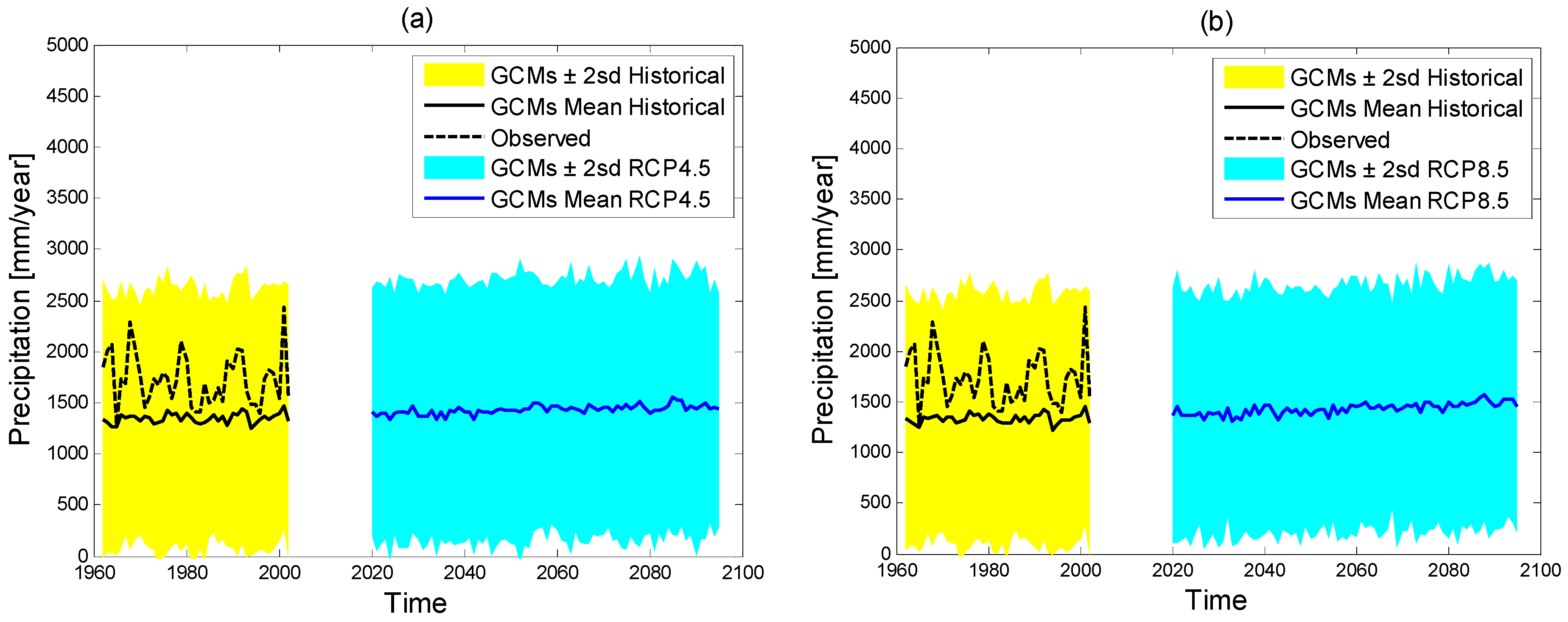
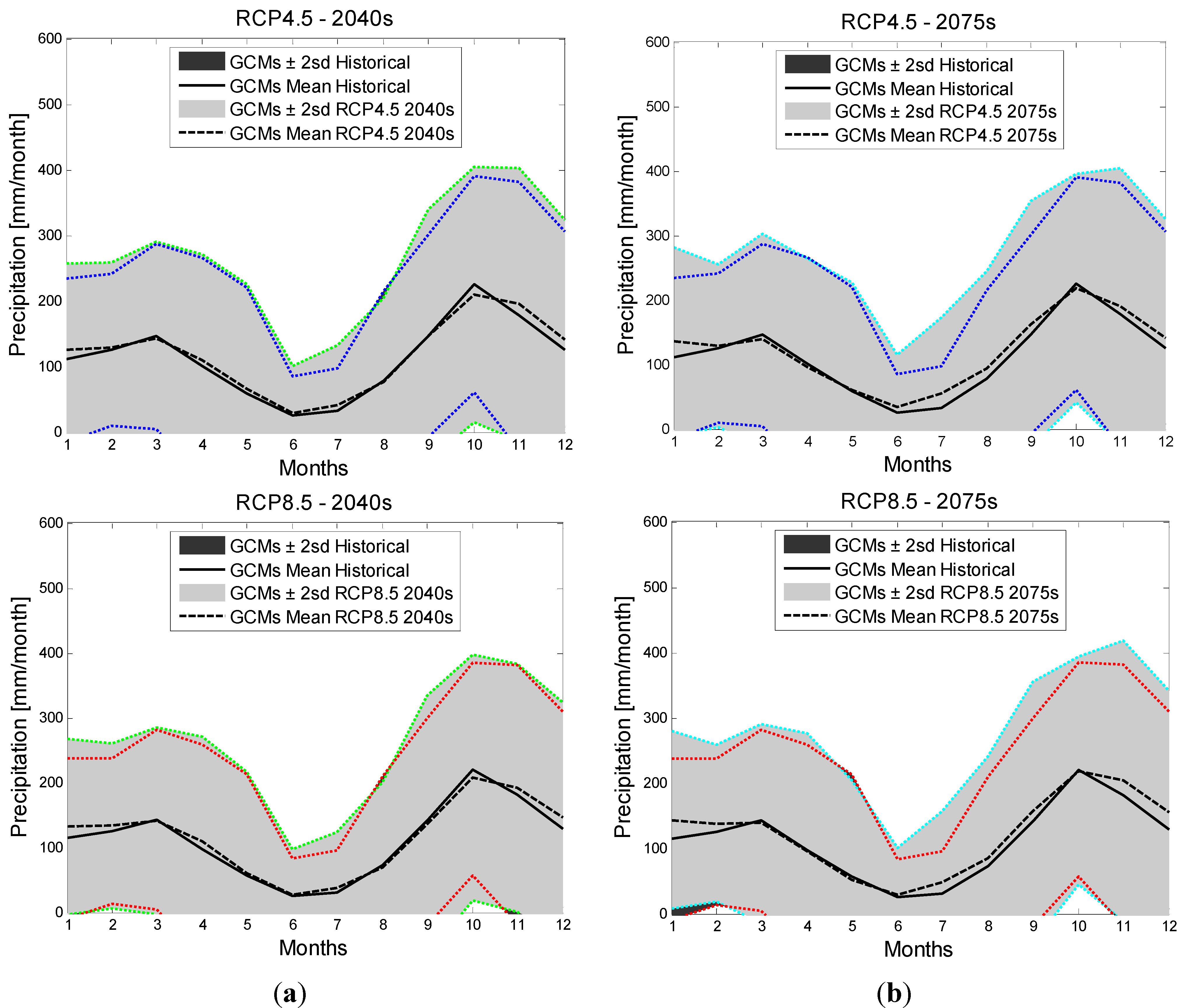
3.2. Analysis of Projected Future Precipitation by GCMs

3.2.1. Monthly, Seasonal and Annual Precipitation

The analysis of projected future changes in rainfall shows no significant change for the average monthly precipitation in the 2040s, but a slight increase for the 2075s especially towards the end of the shorter OND rainy season (Figure 10). The historical analysis described earlier in Section 3.1 showed that the precipitation in the OND season is well captured by the GCMs. The magnitude of change is slightly higher for RCP8.5 under which the temperature increase is higher, leading to higher evapotranspiration and precipitation. The effect of GCM uncertainty is found to be far greater than that due to precipitation simulations between the RCP8.5 and RCP4.5 scenarios (Figure 10). Uncertainties in the future simulations are higher for the 2075s than for the 2040s as scenario uncertainty attributed to the uncertainty in emissions of greenhouse gases—hence radiative forcing increases exponentially especially after the 2060s [26].
Perturbation factors for annual precipitation due to climate change are shown in Figure 11. Generally annual precipitation changes converge to the same level for precipitation of return periods greater than two years. For that reason and to simplify the presentation of results, the mean change is computed for the precipitation extremes and plotted for all GCMs in box plots (Figure 11a). Precipitation extremes are defined as events that are larger or equal to those that occur at least once a year. The lower resolution GCMs like IPSL-CM5A-LR, IPSL-CM5B-LR, BNU-ESM, GFDL-ESM2G and GFDL-ESM2M show higher precipitation changes and mostly positive, while the higher resolution GCMs like CNRM-CM5, BCC-CSM1.1m and MIROC5 show precipitation crowding around the unchanged mean climate.
Figure 10. Seasonal variation of average monthly precipitation for observed and GCM historical, RCP4.5 and RCP8.5 series for (a) 2040s; (b) 2075s. The colored dotted lines indicate the extent of twice the historical standard deviation.
Water 06 02634 g010
Figure 11 shows an increase in annual precipitation over Lake Victoria in the 21st century for both RCP4.5 and RCP8.5 scenarios (only RCP8.5 shown). For the 2040s, annual precipitation is projected to increase by about 7% for both scenarios, while for the 2075s it is expected to increase by about 10% for the RCP4.5 scenario, and more than 15% for the RCP8.5 scenario. Next to this analysis of annual precipitation, summations of precipitation in the MAM, OND and JJAS seasons were analyzed to determine the perturbation factors for the 2040s and 2075s in order to understand the effect of seasonal precipitation on annual precipitation over the Lake Victoria basin. Figure 12 shows the seasonal change factors for RCP8.5 scenario. Most GCMs generally agree well in the OND rainy season as depicted by the lower divergence and narrower box limits for all resolutions (Figure 12a). Precipitation amounts generally increase in all the seasons for the mitigation RCP4.5 scenario. However, for the RCP8.5 scenario, the seasonal amounts increase only in the rainy seasons (Figure 12a). For the dry JJAS season in RCP8.5 scenario, the total seasonal precipitation amount is expected to decrease by about 10% in the 2040s, and increase by about 20% in the 2075s.
Figure 11. (a) Perturbation factors for annual precipitation using events with return periods greater than two years for the different GCMs, for the 2040s (notched) and 2075s for RCP8.5; (b) Perturbation factors vs. return period for annual precipitation for the different GCM simulations for the 2075s under RCP8.5 scenario: Red = LR GCMs, Blue = HR GCMs and Green = MR GCMs.
Water 06 02634 g011
Figure 12. (a) Perturbation factors for total seasonal precipitation simulated by the different GCMs for the 2040s (notched) and 2075s, for RCP8.5; (b) Perturbation factors vs. return period for total seasonal precipitation simulated by the different GCMs in the 2075s for RCP8.5, Red = LR GCMs, Blue = HR GCMs and Green = MR GCMs.
Water 06 02634 g012

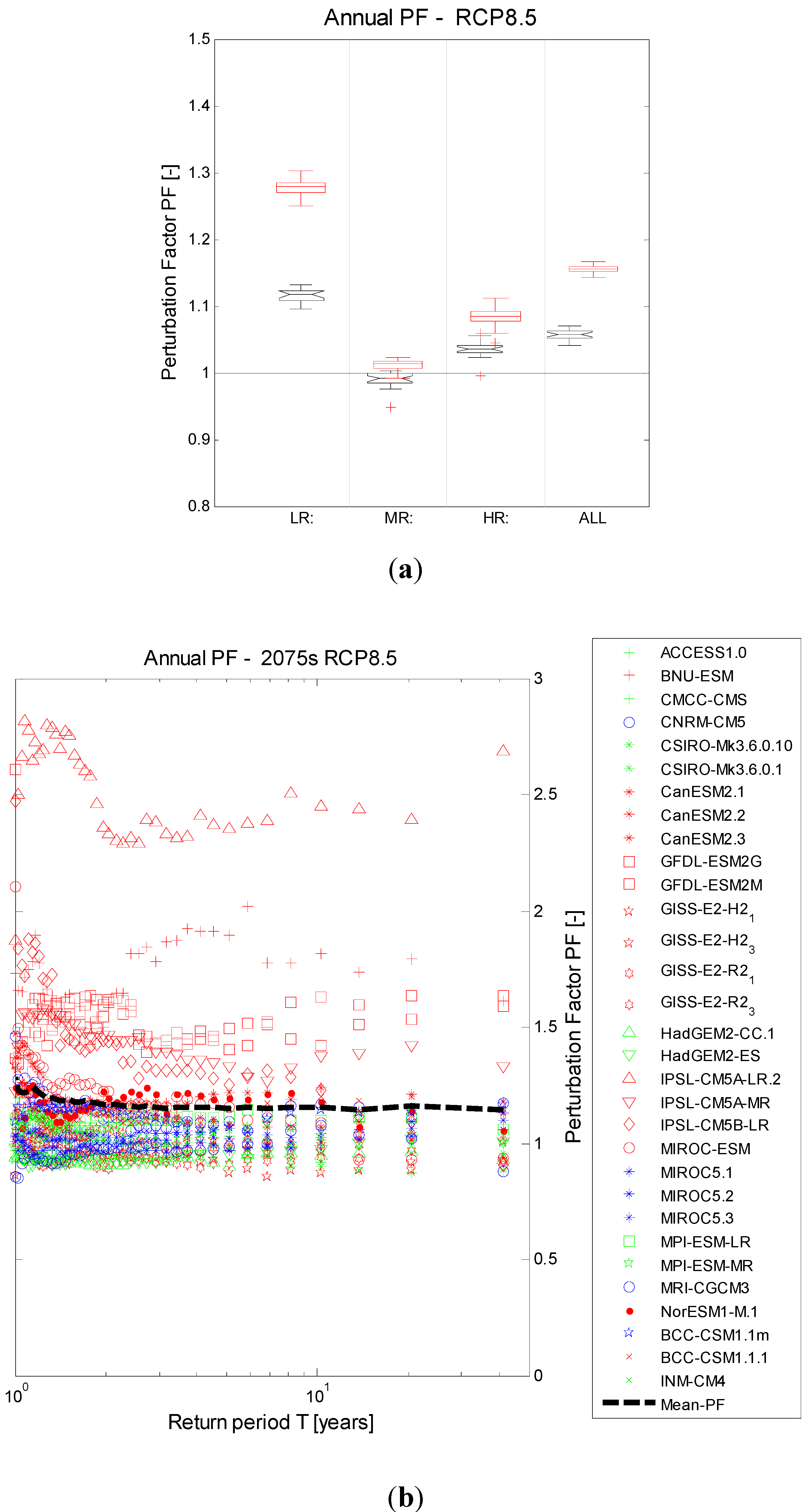
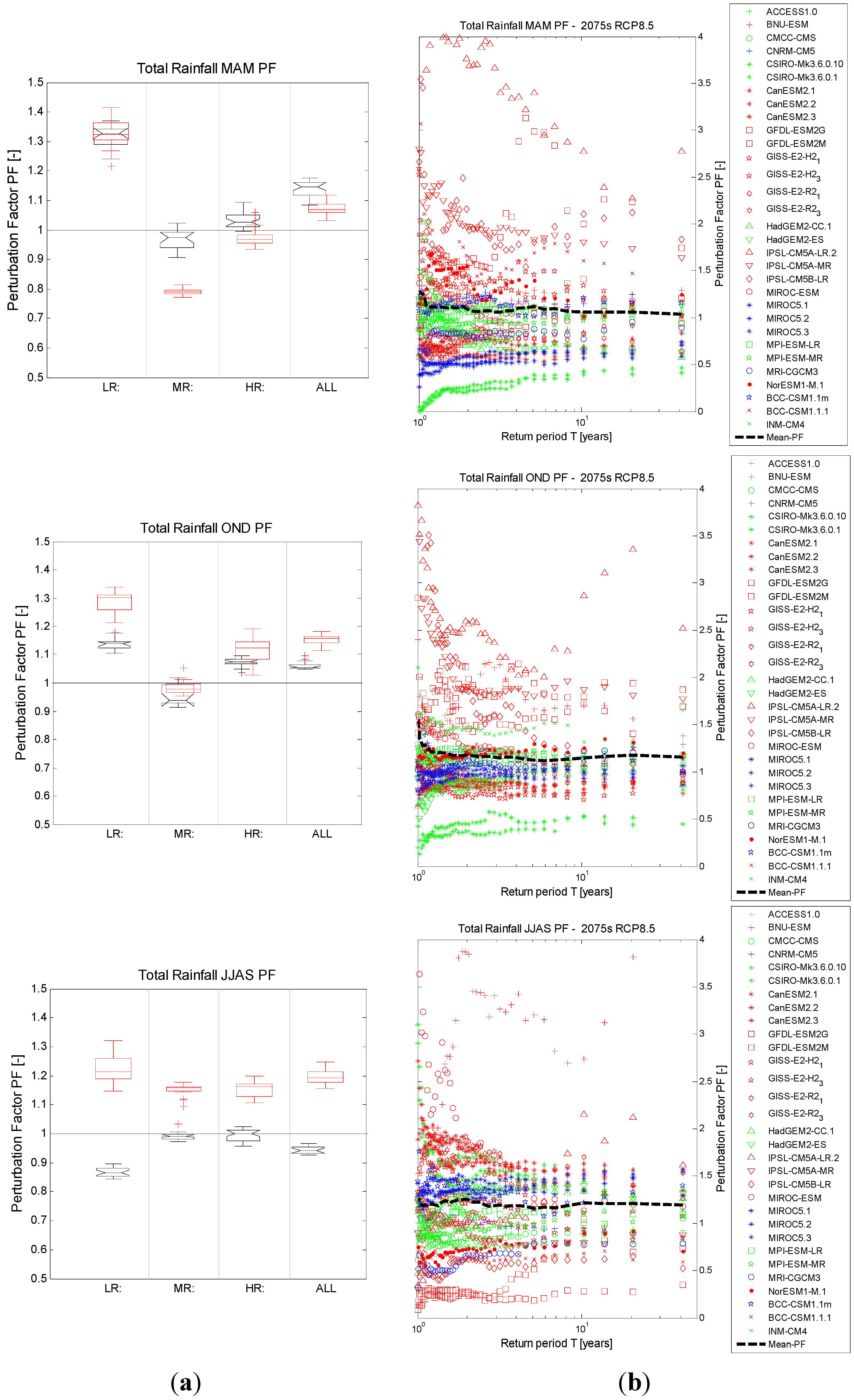
3.2.2. Precipitation Extremes

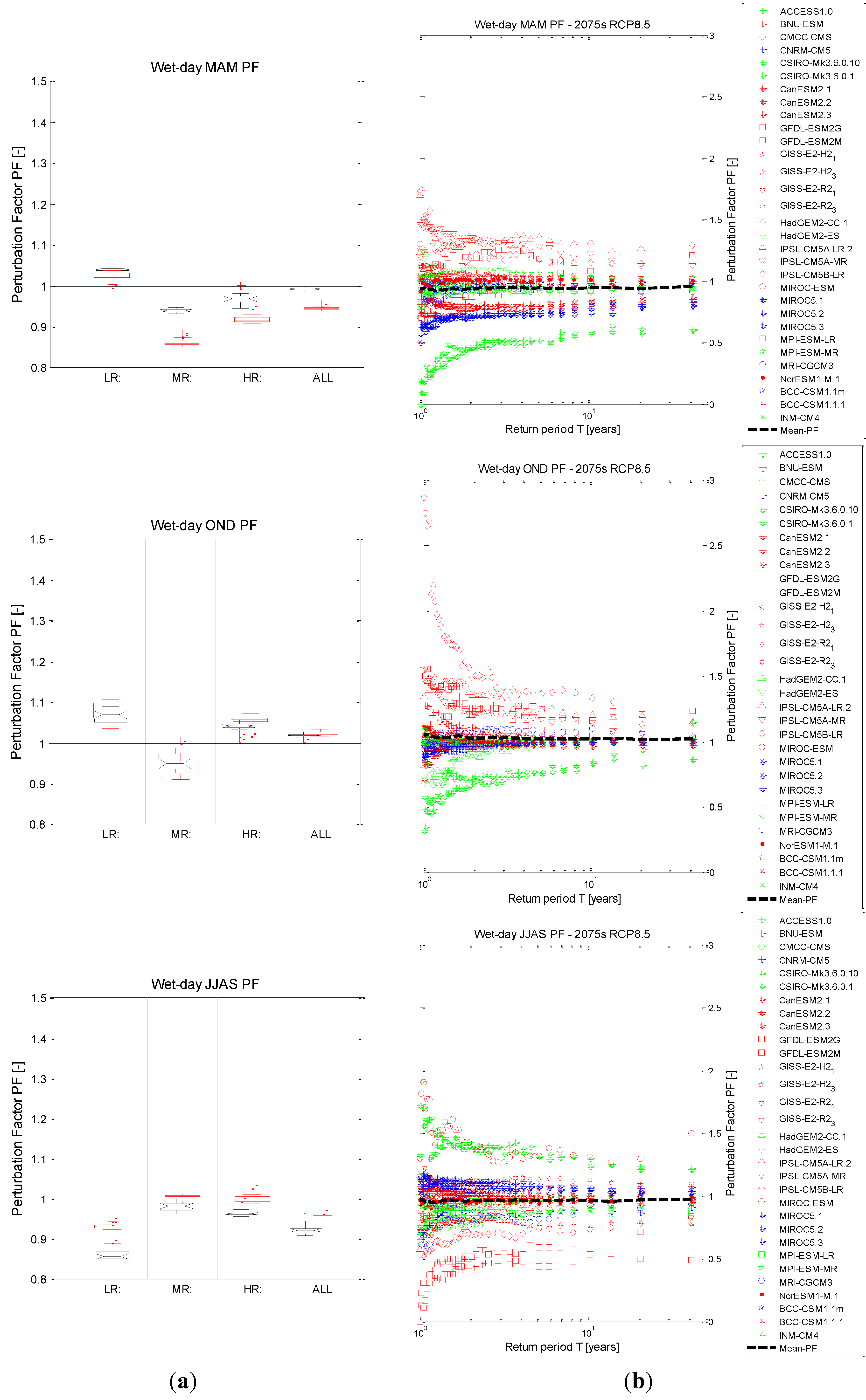
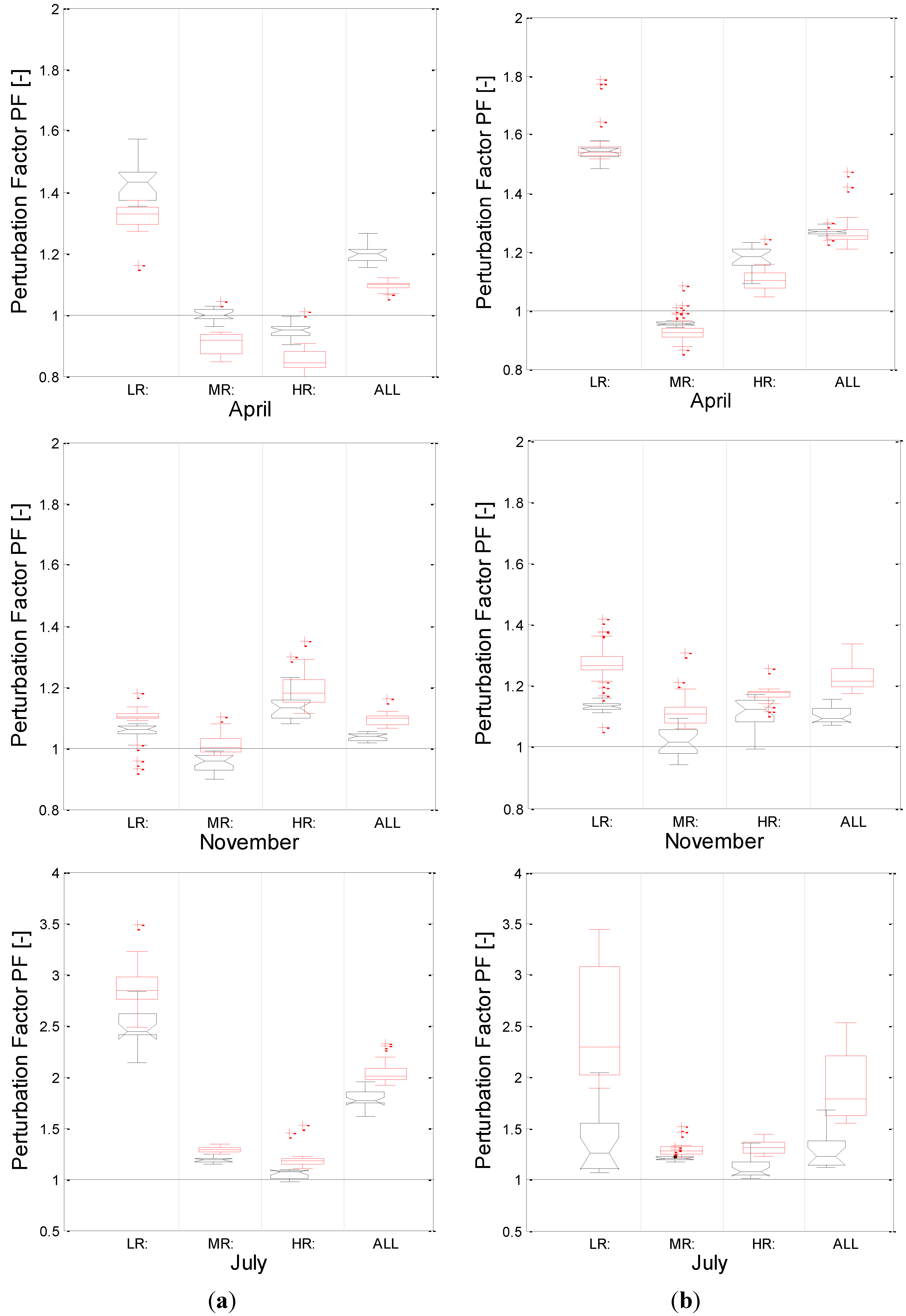
Changes in Number of Wet Days

A wet day is defined as that having intensity greater than 0.1 mm/day. Precipitation volumes are affected by both the number of wet days and the intensity of precipitation. The number of wet days in the historical and future scenarios was obtained for the different seasons to determine the relative changes in the wet day frequency (Figure 13).
Figure 13. (a) Perturbation factors for number of wet days simulated by GCMs in the different seasons for the 2040s (notched) and 2075s, for RCP8.5; (b) Perturbation factors vs. return period for number of wet days simulated by the GCMs in the 2075s for RCP8.5 in different seasons, Red = LR GCMs, Blue = HR GCMs and Green = MR GCMs.
Water 06 02634 g013
The number of wet days decreases in the MAM and JJAS seasons but slightly increases in the OND rainy season for both RCP4.5 and RCP8.5 scenarios (Figure 13). The LR GCMs project greater changes in the number of wet days for the rainy MAM and OND seasons but simulate lower number of wet days in the dry JJAS season probably because larger areas even out localized low precipitation intensities. Annual precipitation over Lake Victoria is estimated to be about 26% higher than over land. This is expected to be associated with 20%–30% more occurrences of cold cloud tops over the lake [27]. It implies that averaging over large areas including land is bound to reduce the precipitation over the lake and sometimes the number of wet days especially in the dry seasons. This again confirms that GCM parameterization and resolution have an important effect on GCM outputs.

Changes in Wet Day Intensities

The daily precipitation intensities in the MAM, OND and JJAS seasons were analyzed to determine the change factors in the 2040s and 2075s under the different scenarios. Figure 14a shows the changes in daily precipitation intensities for the different seasons for events with return periods greater than two years. When changes in wet day intensities vs. return periods are analyzed, the intensities are generally seen to increase in the rainy seasons for both RCP4.5 and RCP8.5 scenarios. The daily precipitation extremes increase more towards the 2075s compared to the 2040s especially for RCP8.5 (Figure 14). However, for the dry JJAS season in the RCP8.5 scenario, daily precipitation is generally expected to remain constant in the 2040s and increase by more than 20% in the 2075s explaining the reason for the decrease in the JJAS seasonal precipitation in the 2040s, and increase in the 2075s (Figure 12). The number of wet days slightly decreases in the dry seasons for both decades yet daily precipitation intensities seem to increase more in the late century than the mid-century. In the 2040s, the RCP8.5 and RCP4.5 projections anticipate similar changes in daily extreme precipitation. The difference in relative forcing for the two scenarios in the 2040s is 1 Wm−2 compared to 3 Wm−2 in the 2075s (Figure 3). This relative difference is consistent with higher temperatures in the 2075s that encourage formation of heavier intense convective storms in the dry season as more moisture is stored in the atmosphere. Therefore, RCP8.5 suggests fewer but heavier intense storms in the 2075s if carbon emissions are not controlled.
Figure 14. (a) Perturbation factors for daily precipitation simulated by GCMs in different seasons for the 2040s (notched) and 2075s, for RCP8.5; (b) Perturbation factors vs. return period for daily precipitation simulated by the GCMs in the 2075s for RCP8.5 in the different seasons, Red = LR GCMs, Blue = HR GCMs and Green = MR GCMs.
Water 06 02634 g014
Most models show an increase in daily precipitation intensities for the dry JJAS season with some LR GCMs like GFDL-ESM2G, GFDL-ESM2M and IPSL-CM5A-LR strongly deviating from the mean change (Figure 14b). The difference in GCM performance are larger in the JJAS and MAM seasons—which were not well captured by the GCMs. Daily precipitation intensities are expected to increase by about 10%–25% in the OND season, which is consistent with the 10%–20% increase in total precipitation for that season (Figure 12). Despite the 10%–15% increase in MAM daily extremes, seasonal volumes increase by less than 10% in the same season since the number of wet days generally decreases in this season (Figure 13). Notwithstanding, in reality this increment is not expected to have any significant influence on the annual precipitation volumes especially since precipitation in the MAM season is generally underestimated by the GCMs as explained in Section 3.1.
Daily precipitation intensities were also checked in the wettest months (April and November) and dry July month (Figure 15). The large spread of the perturbation factor quartiles in the dry month of July is attributed to division by very low historical rainfall amounts especially for LR GCMs that provide precipitation results averaged over larger areas (Figure 15). The resolutions of the GCMs affect the GCM output so care ought to be taken when choosing GCMs for climate change impact projections. LR GCMs show very large variations from the mean change while the HR GCMs values are crowded around the mean. The large variations are even more pronounced for the RCP8.5 scenario. The large uncertainty in the GCM output for LR models is carried into the computed value for the mean change especially visible in the dry month of July (Figure 15), even when mean change often coincides with the results from the HR GCMs suggesting that finer resolution GCMs are favorable in predicting climate change scenarios.
Figure 15. Perturbation factors for daily precipitation simulated by GCMs in the months of April, November and July for the 2040s (notched) and 2075s, including outliers represented by (+) (a) RCP4.5; (b) RCP8.5.
Water 06 02634 g015

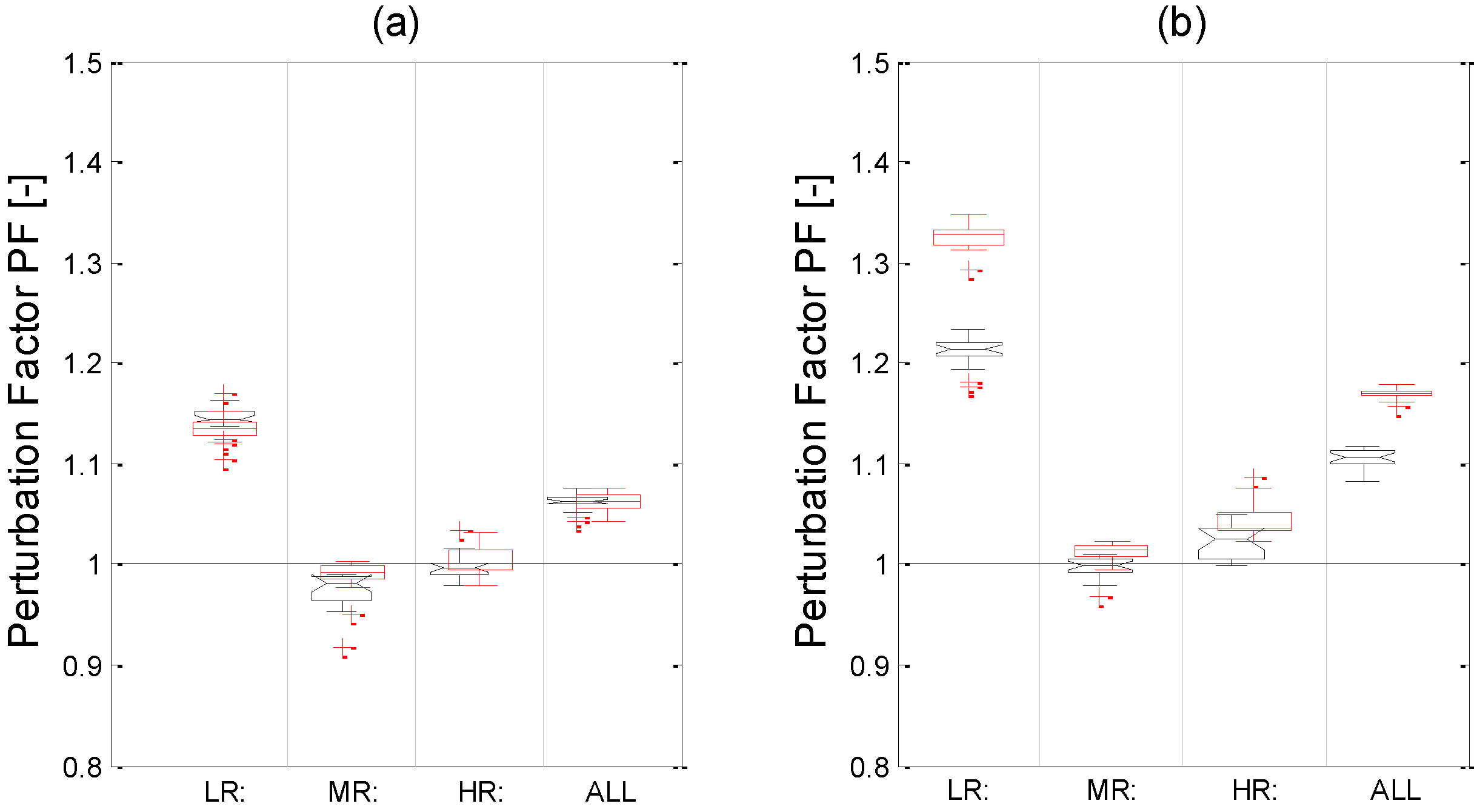
3.3. RCP4.5 vs. RCP8.5 and 2040s vs. 2075s Comparison

Figure 16 and Figure 17 summarize the differences in GCM results for the different scenarios and periods based on their resolutions. Precipitation will generally increase in the 21st century for both RCP4.5 and RCP8.5 scenarios—higher increase is generally anticipated for RCP8.5 compared to RCP4.5 (Figure 16). For RCP4.5, annual precipitation is expected to increase by about 7% for both 2040s and 2075s, while RCP8.5 projects about 10% increase in the 2040s and about 18% in the 2075s. This increase is generally attributed to increased precipitation intensities rather than the total number of wet days, as heavier intense storms are expected in the late 21st century according to Section 3.2. The results are consistent with the positive shift in precipitation distribution expected in other parts of East Africa under global warming for the CMIP3 climate models [28]. Generally, the increase in precipitation is more for the 2075s than for 2040s; and this effect is even greater than that arising from differences between RCP8.5 and RCP4.5 scenarios (Figure 17). A high level of uncertainty is presented by the LR GCMs (grid size >2°) compared to the HR and MR GCMs (Figure 17a,b).
Figure 16. Comparison of mean perturbation factors for annual precipitation based on GCM resolutions for the 2040s (notched) and 2075s, (a) RCP4.5; (b) RCP8.5.
Water 06 02634 g016
Figure 17. Annual precipitation perturbation factors, (a) RCP8.5 vs. RCP4.5, for the 2040s (o) and 2075s (+); (b) 2075s vs. 2040s for RCP4.5 (Δ) and RCP8.5(x), Red = LR GCMs, Blue = HR GCMs and Green = MR GCMs.
Water 06 02634 g017

4. Conclusions

The GCM performance over Lake Victoria is highly dependent on the resolution of the GCM, especially the latitudinal scale. High resolution GCMs, namely CNRM-CM5, MIROC5, HadGEM2-CC, HadGEM2-ES and BCC-CSM1.1m gave the best performance in modeling past absolute precipitation over Lake Victoria. Lower resolution GCMs (grid size >2.5°) e.g., GFDL-ESM2G, GFDL-ESM2M, IPSL-CM5A-LR, IPSL-CM5B-LR and HadCM3 produced larger uncertainties in precipitation simulations. Therefore, for future projections of precipitation, high resolution GCMs are favored to provide reliable seasonal results. However, there is need to use a wide range of GCMs, irrespective of their resolution in order to sufficiently capture the uncertainty in climate modeling physics. This uncertainty may be large as also shown in this paper; hence needs to be taken into account in hydrological impact investigations of climate change.
The total annual precipitation is expected to increase by about 6%–8% for the RCP4.5 scenario and about 10%–18% for the RCP8.5 scenario over the 21st century, despite the higher (up to 40%) increase in extreme daily intensities since the number of wet days does not significantly change. This increase is expected to be higher in the late 21st century (2075s) than in the 2040s.
To study future lake level changes, next to precipitation over the lake, also discharges of main inflowing rivers need to be studied. This requires future projections of precipitation and potential evapotranspiration over the Lake Victoria Basin river subcatchments, and impact modeling by means of catchment runoff models. This research provided the baseline for such study by conducting GCM evaluations in precipitation simulation and analysis of future projections.

Acknowledgments

The authors would like to thank the Vlaamse Interuniversitaire Raad—Institutional University Cooperation (VLIR-IUC) of Belgium for funding this research under the VLIR-ICP PhD program. We also would like to thank the Ministry of Water and Environment, Uganda, and CMIP5 project for availing the data for this research. The performance evaluations in this study are based on the daily CMIP5 model output, obtained through the Program for Climate Model Diagnosis Intercomparison (PCMDI) portal of the Earth System Grid Federation [29]. We also acknowledge use of the precipitation series dataset provided by Michael Kizza. We thank the anonymous reviewers for their constructive comments that tremendously improved the quality of this paper.

Author Contributions

Patrick Willems and Charles B. Niwagaba supervised the PhD research and reviewed this paper contributing to the write-up.

Conflicts of Interest

The authors declare no conflict of interest.

References

  1. Kite, G.W. Recent changes in level of Lake Victoria/Récents changements enregistrés dans le niveau du Lac. Hydrol. Sci. J. 1981, 26, 233–243. [Google Scholar]
  2. Kite, G.W. Analysis of Lake Victoria levels. Hydrol. Sci. J. 1982, 27, 99–110. [Google Scholar] [CrossRef]
  3. Piper, B.S.; Plinston, D.T.; Sutcliffe, J.V. The water balance of Lake Victoria. Hydrol. Sci. J. 1986, 31, 25–37. [Google Scholar] [CrossRef]
  4. Yin, X.; Nicholson, S.E. The water balance of Lake Victoria. Hydrol. Sci. J. 1998, 43, 789–811. [Google Scholar] [CrossRef]
  5. Tate, E.; Sutcliffe, J.; Conway, D.; Farquharson, F. Water balance of Lake Victoria: Update to 2000 and climate change modelling to 2100/Bilan hydrologique du Lac Victoria: Mise à jour jusqu’en 2000 et modélisation des impacts du changement climatique jusqu’en 2100. Hydrol. Sci. J. 2004, 49. [Google Scholar] [CrossRef]
  6. Awange, J.L.; Ogalo, L.; Bae, K.-H.; Were, P.; Omondi, P.; Omute, P.; Omullo, M. Falling Lake Victoria water levels: Is climate a contributing factor? Clim. Change 2008, 89, 281–297. [Google Scholar] [CrossRef]
  7. Swenson, S.; Wahr, J. Monitoring the water balance of Lake Victoria, East Africa, from space. J. Hydrol. 2009, 370, 163–176. [Google Scholar] [CrossRef]
  8. Intergovernmental Panel on Climate Change (IPCC). CLIMATE CHANGE 2013: The Physical Science Basis. Contribution of Working Group I to the Fifth Assessment Report of the Intergovernmental Panel on Climate Change; Cambridge University Press: Cambridge, United Kingdom and New York, NY, USA, 2013; p. 1535. [Google Scholar]
  9. Nicholson, S.E. A review of climate dynamics and climate variability in Eastern Africa. In Limnology, Climatology and Paleoclimatology of the East African Lakes; Johnson, T.C., Odada, E.O., Eds.; Gordon and Breach Publishers: Amsterdam, The Netherlands, 1996; pp. 25–56. [Google Scholar]
  10. Indeje, M.; Semazzi, F.H.M.; Ogallo, L.J. ENSO signals in East African rainfall seasons. Int. J. Climatol. 2000, 20, 19–46. [Google Scholar] [CrossRef]
  11. Nicholson, S.E.; Yin, X. Rainfall conditions in Equatorial East Africa during the Nineteeenth century as inferred from the record of Lake Victoria. Clim. Chang. 2001, 48, 387–398. [Google Scholar] [CrossRef]
  12. Kizza, M.; Rodhe, A.; Xu, C.-Y.; Ntale, H.K.; Halldin, S. Temporal rainfall variability in the Lake Victoria Basin in East Africa during the twentieth century. Theor. Appl. Climatol. 2009, 98, 119–135. [Google Scholar] [CrossRef]
  13. Sene, K.J.; Plinston, D.T. A review and update of the hydrology of Lake Victoria in East Africa. Hydrol. Sci. J. 1994, 39, 47–63. [Google Scholar] [CrossRef]
  14. Mutenyo, I.B. Impacts of Irrigation and Hydroelectric Power Developments on the Victoria Nile in Uganda School. Ph.D. Thesis, Cranfield University, Cranfield, UK, 2009; p. 258. [Google Scholar]
  15. Sutcliffe, J.; Parks, Y. The Hydrology of the Nile; International Association of Hydrological Sciences IAHS: Wallingford, UK, 1999; Volume 5. [Google Scholar]
  16. Kizza, M. Uncertainty Assessment in Water Balance Modelling for Lake Victoria. Ph.D. Thesis, Makerere University Kampala, Kampala, Uganda, 2012. [Google Scholar]
  17. Taylor, K.E.; Stouffer, R.J.; Meehl, G.A. An overview of CMIP5 and the experiment design. Bull. Am. Meteorol. Soc. 2012, 93, 485–498. [Google Scholar] [CrossRef]
  18. Taye, M.T.; Ntegeka, V.; Ogiramoi, N.P.; Willems, P. Assessment of climate change impact on hydrological extremes in two source regions of the Nile River Basin. Hydrol. Earth Syst. Sci. 2011, 15, 209–222. [Google Scholar] [CrossRef]
  19. Nyeko-Ogiramoi, P.; Ngirane-Katashaya, G.; Willems, P.; Ntegeka, V. Evaluation and inter-comparison of Global Climate Models’ performance over Katonga and Ruizi catchments in Lake Victoria basin. Phys. Chem. Earth 2010, 35, 618–633. [Google Scholar] [CrossRef]
  20. Liu, T.; Willems, P.; Pan, X.L.; Bao, A.M.; Chen, X.; Veroustraete, F.; Dong, Q.H. Climate change impact on water resource extremes in a headwater region of the Tarim basin in China. Hydrol. Earth Syst. Sci. 2011, 15, 3511–3527. [Google Scholar] [CrossRef]
  21. Christensen, J.; Kjellström, E.; Giorgi, F.; Lenderink, G.; Rummukainen, M. Weight assignment in regional climate models. Clim. Res. 2010, 44, 179–194. [Google Scholar] [CrossRef]
  22. Shongwe, M.E.; van Oldenborgh, G.J.; van den Hurk, B.; van Aalst, M. Projected changes in mean and extreme precipitation in Africa under global warming. Part II: East Africa. J. Clim. 2011, 24, 3718–3733. [Google Scholar] [CrossRef]
  23. Ntegeka, V.; Baguis, P.; Roulin, E.; Willems, P. Developing tailored climate change scenarios for hydrological impact assessments. J. Hydrol. 2014, 508, 307–321. [Google Scholar] [CrossRef]
  24. Kizza, M.; Westerberg, I.; Rodhe, A.; Ntale, H.K. Estimating areal rainfall over Lake Victoria and its basin using ground-based and satellite data. J. Hydrol. 2012, 464–465, 401–411. [Google Scholar] [CrossRef]
  25. Shaffrey, L.C.; Stevens, I.; Norton, W.A.; Roberts, M.J.; Vidale, P.L.; Harle, J.D.; Jrrar, A.; Stevens, D.P.; Woodage, M.J.; Demory, M.E.; et al. HiGEM: The New U.K. High-Resolution global environment model—Model description and basic evaluation. J. Clim. 2009, 22, 1861–1896. [Google Scholar] [CrossRef]
  26. Hawkins, E.; Sutton, R. The potential to narrow uncertainty in regional climate predictions. Bull. Am. Meteorol. Soc. 2009, 90, 1095–1107. [Google Scholar] [CrossRef]
  27. Ba, M.B.; Nicholson, S.E. Analysis of convective activity and its relationship to the rainfall over the rift valley lakes of East Africa during 1983–90 using the meteosat infrared channel. J. Appl. Meteorol. 1998, 37, 1250–1264. [Google Scholar] [CrossRef]
  28. Shongwe, M.E.; van Oldenborgh, G.J.; Hurk, B. Van Den Projected changes in mean and extreme precipitation in Africa under global warming, Part II: East Africa. J. Clim. 2011, 24, 3718–3733. [Google Scholar] [CrossRef]
  29. ESFG ESFG PCMDI. Available online: http://pcmdi9.llnl.gov/esgf-web-fe/live# (accessed on 31 March 2014).

