Article

Enhancing the Predicting Accuracy of the Water Stage Using a Physical-Based Model and an Artificial Neural Network-Genetic Algorithm in a River System

1
Department of Civil and Disaster Prevention Engineering, National United University, Miaoli 36003, Taiwan
2
National Applied Research Laboratories, Taiwan Typhoon and Flood Research Institute, Taipei 10093, Taiwan
*
Author to whom correspondence should be addressed.
Water 2014, 6(6), 1642-1661; https://doi.org/10.3390/w6061642
Submission received: 28 February 2014 / Revised: 14 April 2014 / Accepted: 21 May 2014 / Published: 3 June 2014

Abstract

:
Accurate simulations of river stages during typhoon events are critically important for flood control and are necessary for disaster prevention and water resources management in Taiwan. This study applies two artificial neural network (ANN) models, including the back propagation neural network (BPNN) and genetic algorithm neural network (GANN) techniques, to improve predictions from a one-dimensional flood routing hydrodynamic model regarding the water stages during typhoon events in the Danshuei River system in northern Taiwan. The hydrodynamic model is driven by freshwater discharges at the upstream boundary conditions and by the water levels at the downstream boundary condition. The model provides a sound physical basis for simulating water stages along the river. The simulated results of the hydrodynamic model show that the model cannot reproduce the water stages at different stations during typhoon events for the model calibration and verification phases. The BPNN and GANN models can improve the simulated water stages compared with the performance of the hydrodynamic model. The GANN model satisfactorily predicts water stages during the training and verification phases and exhibits the lowest values of mean absolute error, root-mean-square error and peak error compared with the simulated results at different stations using the hydrodynamic model and the BPNN model. Comparison of the simulated results shows that the GANN model can be successfully applied to predict the water stages of the Danshuei River system during typhoon events.

1. Introduction

Accurate predictions of water stages during high flow periods are critically important for water resources management and flood control operations. Water stage forecasting in a river with tidal effects is among the most important outstanding problems of flood management. It is never an easy task, because to develop a hydrodynamic model, the behavior of the physical processes must be known. Flow conditions in a river with tidal effects are rarely steady or uniform. Hydrodynamic models provide a physical basis for modeling and have the capability to simulate a wide range of flow conditions. Several researchers have developed flood routing hydrodynamic models based on either the one-dimensional dynamic wave equation or the diffusive wave equation. With these approaches, researchers consider the floodplain section of the one-dimensional river channel. Examples of these formulations are given by [1,2,3,4,5,6,7,8,9]. The one-dimensional model can be used to calculate water stages and flow hydrographs, and it is also computationally more efficient than the two-dimensional and three-dimensional models. However, these hydrodynamic models require accurate river geometry data, which may not be available at the desired locations of the rivers. A major disadvantage of using the models is that the parameters are often difficult to determine from the observed data. Because of their impracticality and complexity, extensive experience is necessary to operate and apply these sophisticated hydrodynamic models.
Because of the existing difficulties and challenges in the prediction of water stages using the flood routing hydrodynamic model, a relatively novel computational approach, artificial neural networks (ANNs), which has found wide acceptance in many disciplines, provides an alternative method for one-step-ahead understanding and management of hydrological processes. ANNs are well-suited for this application, because of their informative processing characteristics, such as nonlinearity, parallelism, noise tolerance and learning and generalization capabilities [10,11]. During the last decade, the ANN approach had been widely used for forecasting river flow and stage with greater accuracy. Most studies have shown that if ANN models are trained with a large number of appropriate input data sets, they can yield promising results. Recently, ANNs have been successfully applied in modeling rainfall runoff processes and stream flow [12,13,14,15,16,17,18,19,20,21,22,23,24,25,26,27], as well as predicting the water level in river systems [28,29,30,31,32]. However, few studies have focused on the comparison of ANN models with physically-based models [33]. Demirel et al. [34] have used SWAT (Soil Water Assessment Tool) and ANN models to forecast flow in the Pracana basin, Portugal, and have found that the ANN model is better than the physically-based model in predicting peak flow values. Panda et al. [35] have simulated river stages in the Mahanadi River delta, India, using ANN and the MIKE 11 hydrodynamic model. They found that the performance of the ANN model is better than the MIKE 11 model during the training and testing phases. Chen et al. [36] has compared the ANN model with two-dimensional and three-dimensional hydrodynamic models for simulating estuary water stages. They have found that the ANN approach was more accurate than the two-dimensional and three-dimensional models, because the hydrodynamic models cannot capture the estuary water stage during extreme high flow periods.
In this study, a one-dimensional flood routing hydrodynamic model was used to simulate the water stages in the Danshuei River system in northern Taiwan during typhoon events. Two artificial neural network models were subsequently adopted to improve the calculations of the flood routing hydrodynamic model. Three quantitative statistical measures, i.e., the mean absolute error, root-mean-square error and peak error, were used to evaluate the prediction of water stages during the seven typhoon events using a flood routing hydrodynamic model and two ANN models, including the back propagation neural network (BPNN) and hybrid artificial neural network genetic algorithm (GANN) techniques.

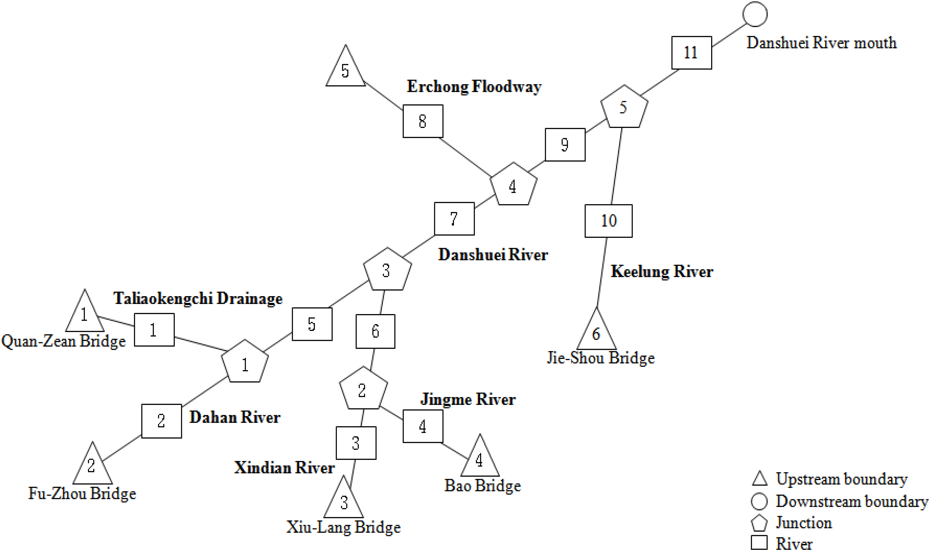
2. Description of the Study Site

The Danshuei River is located in northern Taiwan (Figure 1). It has three major tributaries, the Dahan River, the Xindian River and the Keelung River. The Jingme River and the Taliaokengchi Drainage are tributaries of the Xindia River and the Dahan River, respectively. The corresponding watershed services an area inhabited by more than six million people [37]. The Erchung flood diversion channel, built near the confluence of the Danha River and the Xindian River in 1984, has been used to divert flood flows in the past. The area of the Danshuei watershed is 2726 km2, and the mean annual precipitation is 3001 mm. The total channel length is 327.6 km, and the channel slope ranges from 0.015 to 0.0027. The peak discharges of a 200-year flood are 235.00 m3/s, 103.00 m3/s and 2700 m3/s for the Dahan Stream, the Xindian River and the Keelung River, respectively. The annual mean freshwater discharges at the upstream tidal limits of the Dahan River, the Xindian River and the Keelung River are 62.1 m3/s, 72.7 m3/s and 26.1 m3/s, respectively. The mean tide at the Danshuei River mouth is 2.21 m above the mean sea level. The downstream reaches of all three tributaries are affected by tides [38].
Figure 1. Layout of the Danshuei River system in northern Taiwan. The transect line represents the cross-section.
Water 06 01642 g001

3. Materials and Methods

3.1. Flood Routing Hydrodynamic Model

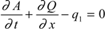
3.1.1. Governing Equations

The flood routing hydrodynamic model is based on the dynamic wave theory of the Saint-Venant equations, which consist of the one-dimensional continuity and momentum equations:
Water 06 01642 i001
Water 06 01642 i002
where, A is the cross-sectional area; Y is the water depth; Q is the discharge; q1 is the lateral inflow per unit channel length; S0 is the channel bottom slope; Sf is the friction slope; V1 is the longitudinal velocity component of the lateral inflow; g is the gravitational acceleration; t is time and x is the distance along the channel. Because the cross-sectional area can be written as a function of water depth, only two flow variables, Q and Y, must be solved in Equations (1) and (2).
The continuity and momentum equations can be solved numerically, given the initial and boundary conditions. There are three conventional numerical approaches, including finite difference, finite element and finite volume methods used to solve one-dimensional continuity and momentum equations. Of the various implicit schemes that have been developed, the “four-point” schemes appear most advantageous, since they can readily be used with unequal distance intervals. Therefore, a four-point implicit finite-difference approximation scheme was used in this study [39,40]. The detailed solutions of the flood routing hydrodynamic model can be found in Hsu et al. [41].

3.1.2. Model Setup

In this study, the model transects were established consistent with the measured cross-sectional profiles at intervals of approximately 0.5 km along the river. The theoretical model transects include 310 transects that cover 11 river reaches (shown in Table 1). The observed data at the upstream and downstream boundary conditions were used to drive the model simulation. The upstream boundaries are specified at the Fu-Zhou Bridge (Dahan River), the Quan-Zean Bridge (Tailiaokengchi Drainage, a tributary of the Dahan River), the Xiu-Lang Bridge (Xindian River), the Bao Bridge (Jingme River, a tributary of the Xindian River) and Jie-Shou (Keelung River). The downstream boundary is at the mouth of the Danshuei River. The upstream and downstream boundaries are shown in Figure 1. The boundary conditions for the dynamic flood routing model at the upstream reaches are the observed hourly discharges, and the observed hourly tide stages are specified at the river mouth (Figure 2). Because the upstream boundaries have been specified with the observed discharges, the rainfall-runoff model to compute runoff discharges did not include the one-dimensional hydrodynamic model.
Table 1. Cross-sectional number of river reaches and Manning friction factor, n, used in the computational domain.
River Reach Number123456
Number of cross-section718313922
Manning friction n0.0250.033~0.0390.033~0.0400.035~0.0450.033~0.0390.030~0.035
River Reach Number7891011
Number of cross-section2210213713
Manning friction n0.022~0.0270.022~0.0300.0250.019~0.0900.023~0.028
Note: the unit of manning friction n is m13 / s.
Figure 2. The Danshuei River system layout for the flood routing hydrodynamic model simulation and boundary conditions.
Water 06 01642 g002

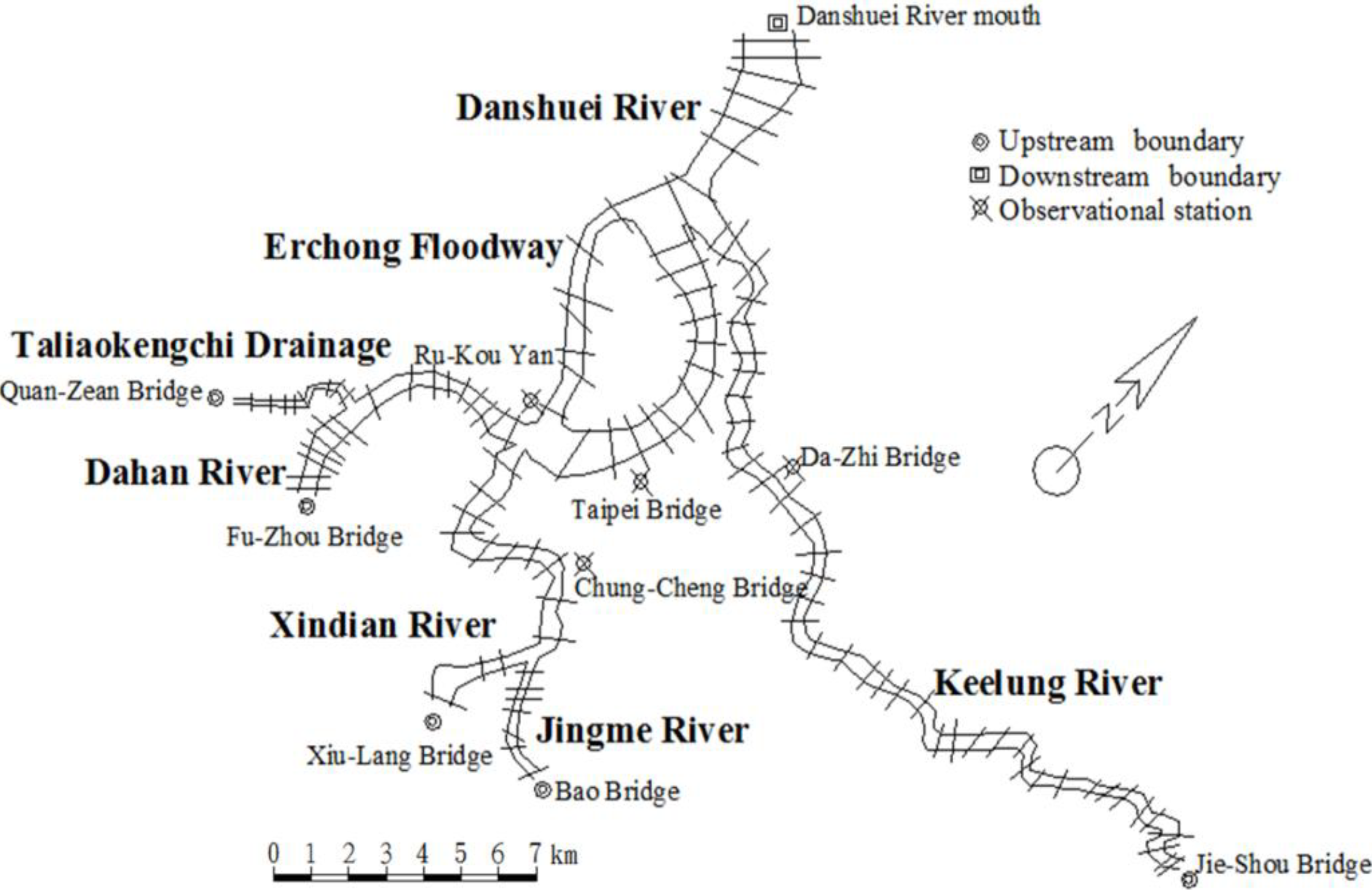
3.2. Artificial Neural Network (ANN) Models

In the present study, two ANN models, including BPNN and GANN, were introduced. The algorithms for these two ANN models are described below.

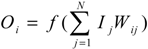
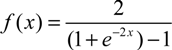
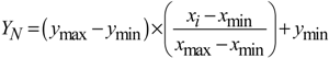
3.2.1. Back Propagation Neural Network (BPNN)

A back propagation neural network (BPNN) was used to amend the simulated water stage results with the one-dimensional flood routing hydrodynamic model to achieve more accurate predictions. The BPNN proposed by Rumelhart et al. [42] is a multiple layer network with nonlinear differentiable transfer functions, including an input layer, a hidden layer and an output layer. Each layer contains a number of neurons. Each neuron receives inputs from neurons in the previous layers or external inputs and converts the input either to an output signal or to another input signal to be used by neurons in the next layers. Connections between neurons in successive layers are assigned weights, which represent the importance of that connection in the network. First, the neurons execute a weighted summation of all inputs and further assess the weighted sum by an activation function, f:
Water 06 01642 i003
where, Oi is the output of neuron i; Ij is the input to the neuron and Wij is the synaptic weight.
In a recent study, Zadeh et al. [43] showed that the tangent sigmoid activation function performed better than the logistic sigmoid activation function in daily outflow prediction when the data was randomly selected. Yonaba et al. [44] endorsed the tangent sigmoid as the most pertinent transfer function for streamflow forecasting, over the bipolar (logistic) and Elliott sigmoids. These two studies indicated the importance of appropriate activation function. The advantage of a tangent sigmoid is proven to be a suitable transfer function, while the disadvantage is that this transfer function needs more computing time. Therefore, a hyperbolic tangential sigmoid transfer function in Equation (4) is used in the hidden layer.
Water 06 01642 i004
A linear transfer function in Equation (5) is applied in the output layer.
f (x) = x
To scale the inputs and the targets, the normalized equation, Equation (6), is often used, forcing the data to fall within a specified range.
Water 06 01642 i005
where, YN is the value after normalization; xmin and xmax are the minimum and maximum values of the data, respectively; and ymin and ymax are −1 and 1, respectively.
The process of training a neural network involves tuning the values of the weights and biases of the network to optimize network performance. Training of the ANN includes minimizing the cost function, C:
Water 06 01642 i006
where, P is the number of input-output training patterns; ek(n) is the difference between the output and target of neuron k for the nth input-output pattern, and M is the number of neurons in the output layer.
The back-propagation method was adopted in the ANN training, utilizing the Levenberg–Marquardt algorithm [45], which seeks to optimize the network parameters and utilizes a non-linear least squares error minimization technique. The Levenberg–Marquardt algorithm combines the ability of the gradient descent method to converge from the starting location, which may be outside the zone of convergence for the Gauss–Newton method, and the speed of the Gauss–Newton method to converge to the solution once the approximate location of the solution has been reached by the gradient descent method. The artificial neural network model was implemented in MATLAB, in which the Levenberg–Marquardt technique is available in the Neural Network Toolbox.

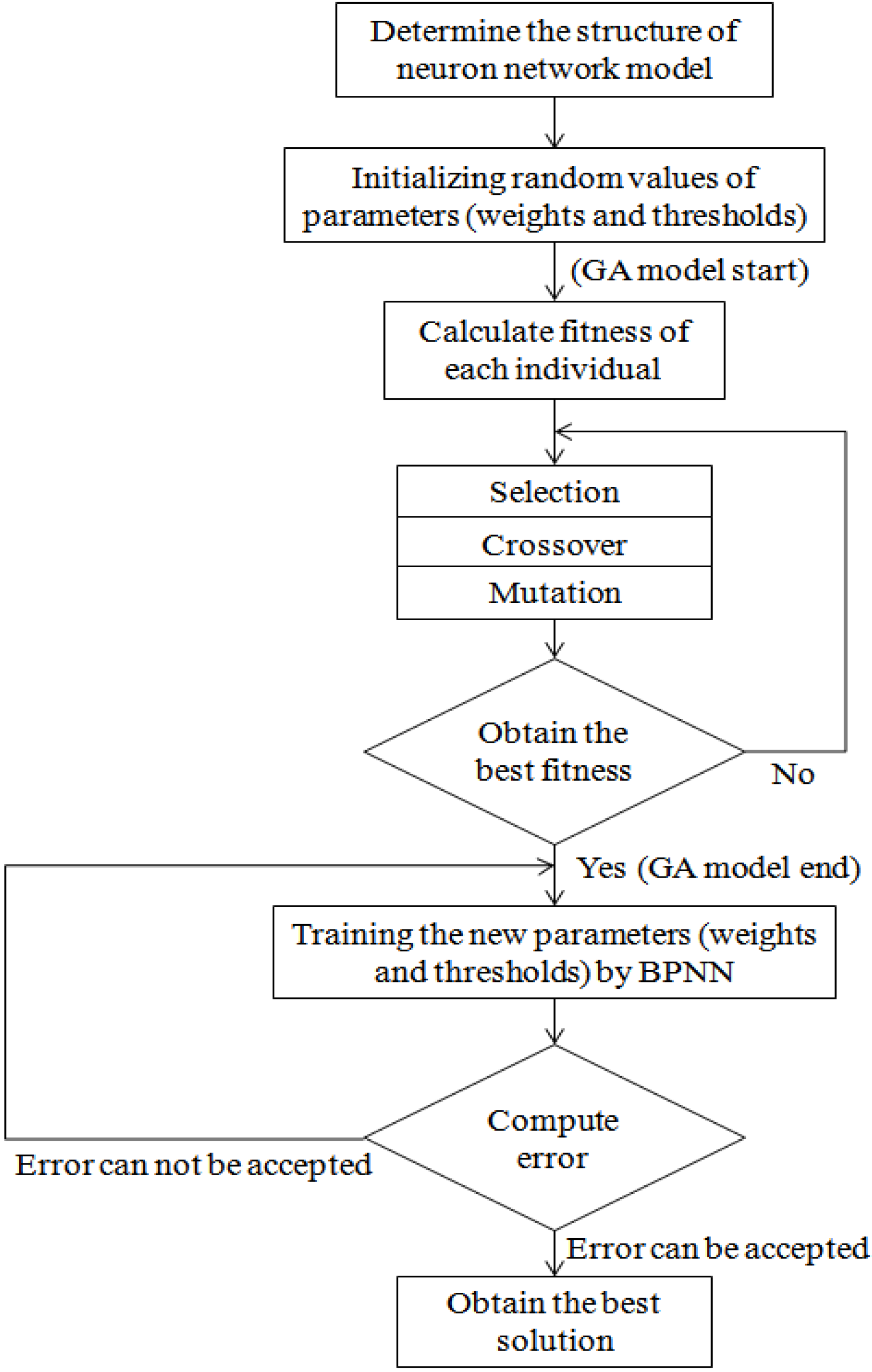
3.2.2. Hybrid Neural Networks and the Genetic Algorithm

ANN training methods provide a non-linear mapping between inputs and outputs and are extremely useful in recognizing patterns in complex data. Methods, such as back-propagation (BP), have been improved with the genetic algorithm technique (GA). The training starts with GA, which executes a global search on the net weight range, refining an initial random set of weights to yield a better value, most likely closer to the global optimum. The BP algorithm then progresses the training, refining the solution provided by GA to approach the optimal solution.
The development of GA was inspired by the basic concepts of Darwinian evolution. It is a heuristic method for solving computationally difficult problems [46]. GA has an advantage over many traditional heuristic methods when search spaces are high modal, discontinuous or constrained. It is the most popular form of evolutionary algorithm used in the diverse field of optimization problems [47]. The algorithm initializes with a population of solutions, known as chromosomes, and transforms itself by three genetic operators, selection, crossover and mutation, to obtain a better solution for the problem after each generation. A fitness function is used to assess the probability of acceptance of individual chromosomes in the next generation. Based on individual fitness values, some chromosomes are selected by elitism and some are selected for the crossover operation. Chromosomes selected for the crossover operation are called the parent solution. After crossover, a set of parents produces two children solutions. The mutation operation introduces random changes in the structure of the population. After performing three genetic operations, fitness values are calculated, and the worst solutions are eliminated from the population, which helps to maintain a constant population size. This one cycle of operation is known as a generation. The population of chromosomes obtained after one generation is the starting solution for the next generation.
In the present study, the fitness values of all these chromosomes were evaluated using the fitness function. Some of the chromosomes were selected by elitism. The probabilistic-selection criterion was applied for selecting chromosomes for the crossover and mutation operation. Some poorly fitted chromosomes were eliminated from the chromosome solution to maintain the population size constant. The initial population size was 50; after each generation, poor solutions were eliminated to maintain a population size. This genetic operation was performed until it reached the maximum generation value. After reaching maximum generation, the model provided a set of final solution. The chromosome corresponding to the minimum error value is the best solution for the model.
The flow chart in Figure 3 shows the proposed method for this study.
Figure 3. Flow chart of the ANN method linked with the GA optimizer. BPNN, back propagation neural network.
Water 06 01642 g003

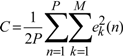
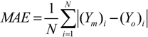
3.2.3. Indices of Simulation Performance

To evaluate the performance of the one-dimensional flood routing hydrodynamic model and the ANN models, three different criteria were considered to compare the predicted results with the observed data, mean absolute error (MAE), root-mean-square error (RMSE) and peak error (PE), based on the following equations:
Water 06 01642 i007
Water 06 01642 i008
Water 06 01642 i009
where, N is the total number of data; Ym is the predicted water stage; Yo is the observed water stage; Ym,peak is the predicted peak water stage and Yo,peak is the observed peak water stage.

4. Results

Seven data sets were used to evaluate the practical accuracy of the models and to ascertain the predictive capability of the models. Five typhoon events, Typhoon Aere (2004), Typhoon Haima (2004), Typhoon Nockten (2005), Typhoon Matsa (2005) and Typhoon Sepat (2007) (673 hourly water stage data), were used for the flood routing hydrodynamic model calibration (and ANN model training), and two typhoon events, Typhoon Fungwong (2008) and Typhoon Morakot (2009) (371 hourly water stage data), were used for flood routing hydrodynamic model verification (and ANN model verification). The calibration and verification events are independent and are not related to each other.

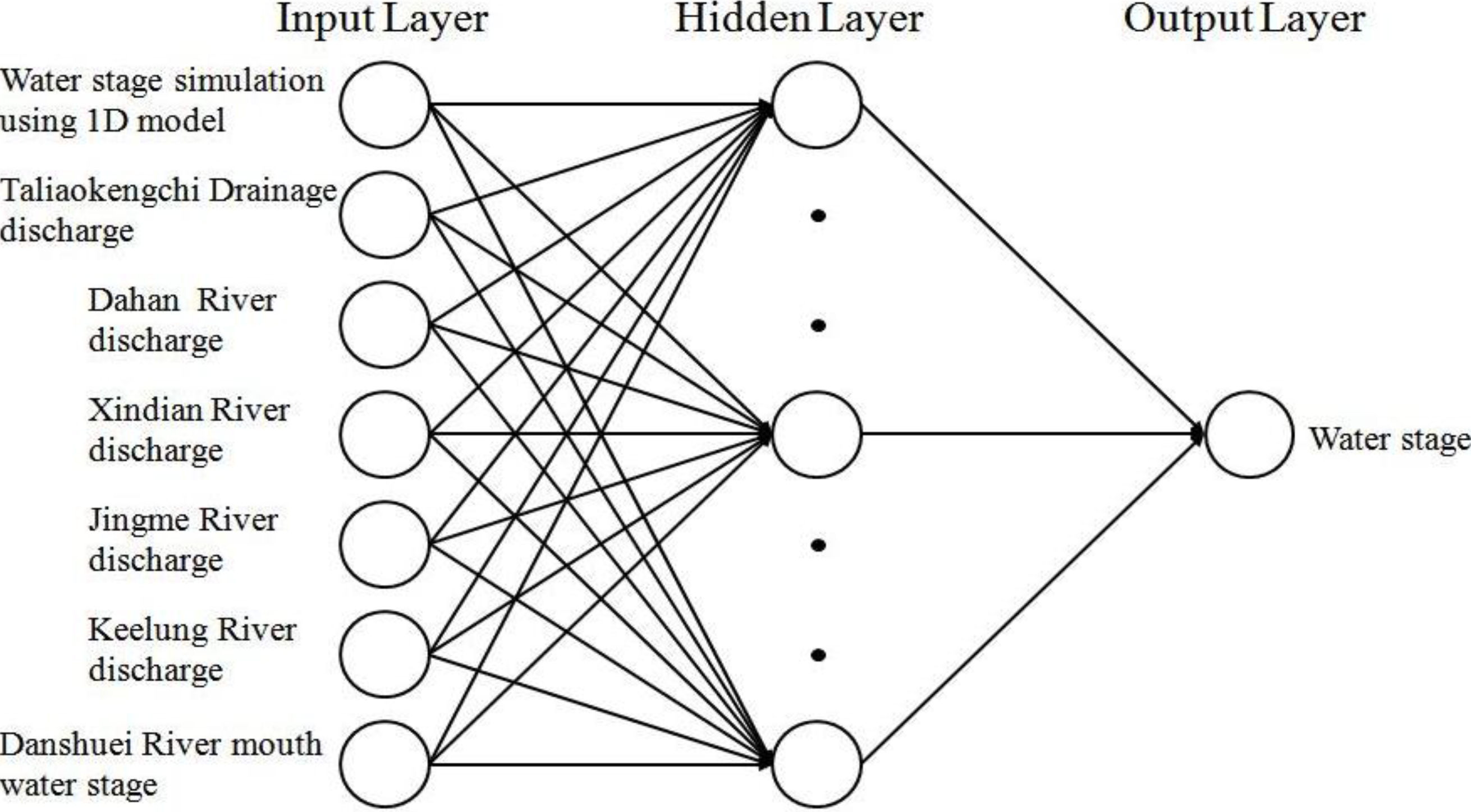
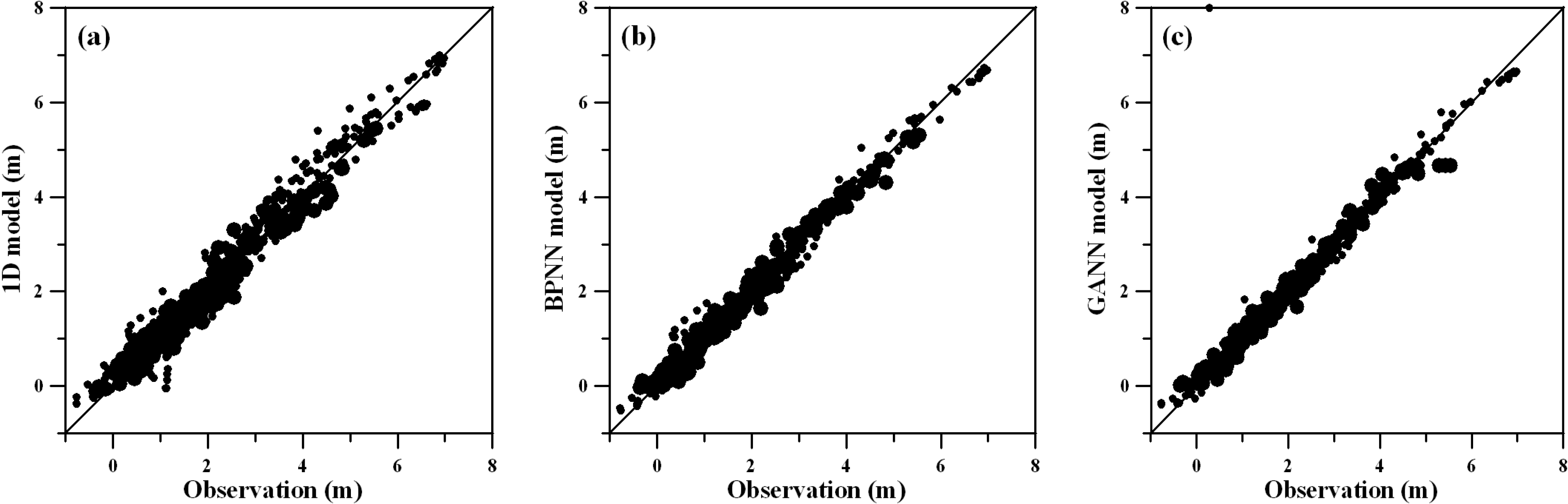
4.1. Flood Routing Hydrodynamic Model Calibration and ANN Model Training

The terminology for model comparisons, i.e., the calibration and verification with the flood routing hydrodynamic model, is used as an analog for the training and verification phases with the ANN model (both BPNN and GANN approaches). The friction coefficient (n) is an important parameter that impacts water stage calculations in the Danshuei River system during floods. The coefficients were tuned in the hydrodynamic model to match the observed water stages at different gauge stations, including the Taipei Bridge, Ru-Kou-Yan, the Chung-Cheng Bridge and the Da-Zhi Bridge.
Figure 4 presents the prediction of the water stage at the Ru-Kou-Yan station by the hydrodynamic model calibration for five typhoon events. The model fails to predict the peak water stage during the high flow period. Table 2 shows the MAE, RMSE and PE for the model calibration at four stations. The maximum MAE, RMSE and PE values for Ru-Kou-Yan are 0.29 m, 0.36 m and 10.87%, respectively. The Manning friction coefficient (n) used in the model is shown in Table 1. A high Manning friction coefficient (n = 0.09) is used at the upstream reaches of the Keelung River, because the channel is composed of large stones [41].
Figure 4. Comparison of observed and simulated water stages for the flood routing hydrodynamic model, BPNN and genetic algorithm neural network (GANN) model calibration at the Ru-Kuo-Yan station for: (a) Typhoon Aere (2004); (b) Typhoon Haima (2004); (c) Typhoon Nockten (2005); (d) Typhoon Matsa (2005); and (e) Typhoon Sepat (2007).
Water 06 01642 g004
Table 2. The performance of the one-dimensional flood routing hydrodynamic model, the BPNN model and the GANN model with respect to predicting water stage during the calibration (training) phase at four stations.
MethodTaipei BridgeRu-Kou-YanChung-Cheng BridgeDa-Zhi Bridge
MAE (m)RMSE (m)PE (%)MAE (m)RMSE (m)PE (%)MAE (m)RMSE (m)PE (%)MAE (m)RMSE (m)PE (%)
Calibration with one-dimensional hydrodynamic model0.260.327.610.290.3610.870.260.355.460.210.268.96
Training with BPNN model0.110.154.770.120.175.000.190.264.090.150.195.41
Training with GANN model0.100.133.070.110.144.190.140.192.810.140.183.16
Notes: MAE, mean solute error; RMSE, root mean square error; PE, peak error.
Because of the poor accuracy in simulating the water stage using the one-dimensional flood routing hydrodynamic model, ANN models, including BPNN and GANN, were employed to improve the water stage calculations. The BPNN structure for predicting water stage is shown in Figure 5. The input layer includes the water stage simulated by the one-dimensional flood routing hydrodynamic model; the upstream discharges of the Taliaokengchi Drainage, the Dahan River, the Xindian River, the Jingme River and the Keelung River; and the water stage at the Danshuei River outlet. The output is the predicted water stage at the gauge stations.
Figure 5. BPNN structures for predicting the water stage.
Water 06 01642 g005
Figure 6a shows the influence of hidden nodes on the RMSE for the BPNN training and the verification phases at the Ru-Kou-Yan station. To obtain the optimal number of nodes in the hidden layer, 14 hidden nodes were chosen during the training and verification phases. Wang et al. [48] identified the optimal number of nodes of the hidden layer using a trial and error procedure by varying the number of hidden nodes. Their study revealed that RMSE values decreased as the number of hidden nodes increased for the training phase, while RMSE values increased as the number of hidden nodes increased for the testing phase. In our case, the RMSE values increase a little as the number of hidden nodes increases for both training and verification phases (Figure 6a). This may be the reason for the different data characteristics, resulting in different results.
Figure 6b shows the relation between the mean square error (MSE) and the number of iterations for Ru-Kou-Yan station. The MSE did not change significantly when the number of iterations exceeded 2300. Therefore, 2500 iterations were adopted for BPNN training and verification. Chen et al. [49] explored an artificial neural network (ANN) model, including the back propagation neural network (BPNN) and adaptive neuro-fuzzy inference system (ANFIS) algorithms used to correct poor calculations with a two-dimensional hydrodynamic model in predicting storm surge height during typhoon events. They found that mean square error decreased with the increasing number of iterations. Similar patterns were also reported by Glose et al. [50]. Table 3 lists the parameters used in the BPNN model.
The prediction of the water stage at the Ru-Kou-Yan station by the BPNN model training for the five typhoon events is also shown in Figure 4. The performance evaluation using the BPNN model for predicting the water stage during the training phase is shown in Table 2. The results show that the BPNN model improves the prediction of the water stage, because the MAE, RMSE and PE using the BPNN model are lower than with the one-dimensional flood routing hydrodynamic model. The maximum values of the MAE, RMSE and PE are 0.19 m and 0.26 m, at the Chung-Cheng Bridge, and 5.41%, at the Da-Zhi Bridge, respectively.
Figure 6. (a) The effect of the number of nodes in the hidden layer on the root-mean-square error (RMSE) at the Ru-Kou-Yan station; and (b) the variation in mean square error (MSE) with iterations.
Water 06 01642 g006
Table 3. The parameters used in the BPNN model.
ParametersTaipei BridgeRu-Kou-YanChung-Cheng BridgeDa-Zhi Bridge
Input nodes7777
Hidden nodes714117
Output nodes1111
Learning rate0.010.010.010.01
Momentum0.70.70.70.7
Iterations2500250025002500
Figure 4 also shows the simulated water stage at the Ru-Kou-Yan station using the GANN model training for the five typhoon events. Table 2 also presents the statistical errors of performance for predicting the water stages at different stations with the GANN model. Based on the simulated results, the configuration of the GA to predict water stages is listed in Table 4 and includes the population size, maximum generation number, crossover probability and mutation probability. These values were defined as a default after several GA studies performed by the researchers with different applications [51,52].
Table 4. The configuration of the GA.
ParametersTaipei BridgeRu-Kou-YanChung-Cheng BridgeDa-Zhi Bridge
Population size30303025
Maximum generation2500250025002500
Crossover probability1.00.91.01.0
Mutation probability0.010.010.010.01
The results in Figure 4 and Table 2 show that the prediction of the water stage with the GANN model is better than with either the one-dimensional flood routing hydrodynamic model or the BPNN model. The maximum MAE, RMSE and PE values for the GANN training phase are 0.14 m and 0.19 m, at Chung-Cheng Bridge, and 4.19%, at Ru-Kou-Yan station, respectively. The scatter plot of simulated and observed water stages using the one-dimensional flood routing hydrodynamic model, the BPNN model and the GANN model for five typhoons and four gauge stations is shown in Figure 7. A comparison of the results shows that the GANN technique is successful in predicting the water stage.
Figure 7. The scatter plots of simulated and observed water stages using (a) the one-dimensional flood routing hydrodynamic model; (b) the BPNN model; and (c) the GANN model for the calibration (training) phase for five typhoon events and four stations.
Water 06 01642 g007

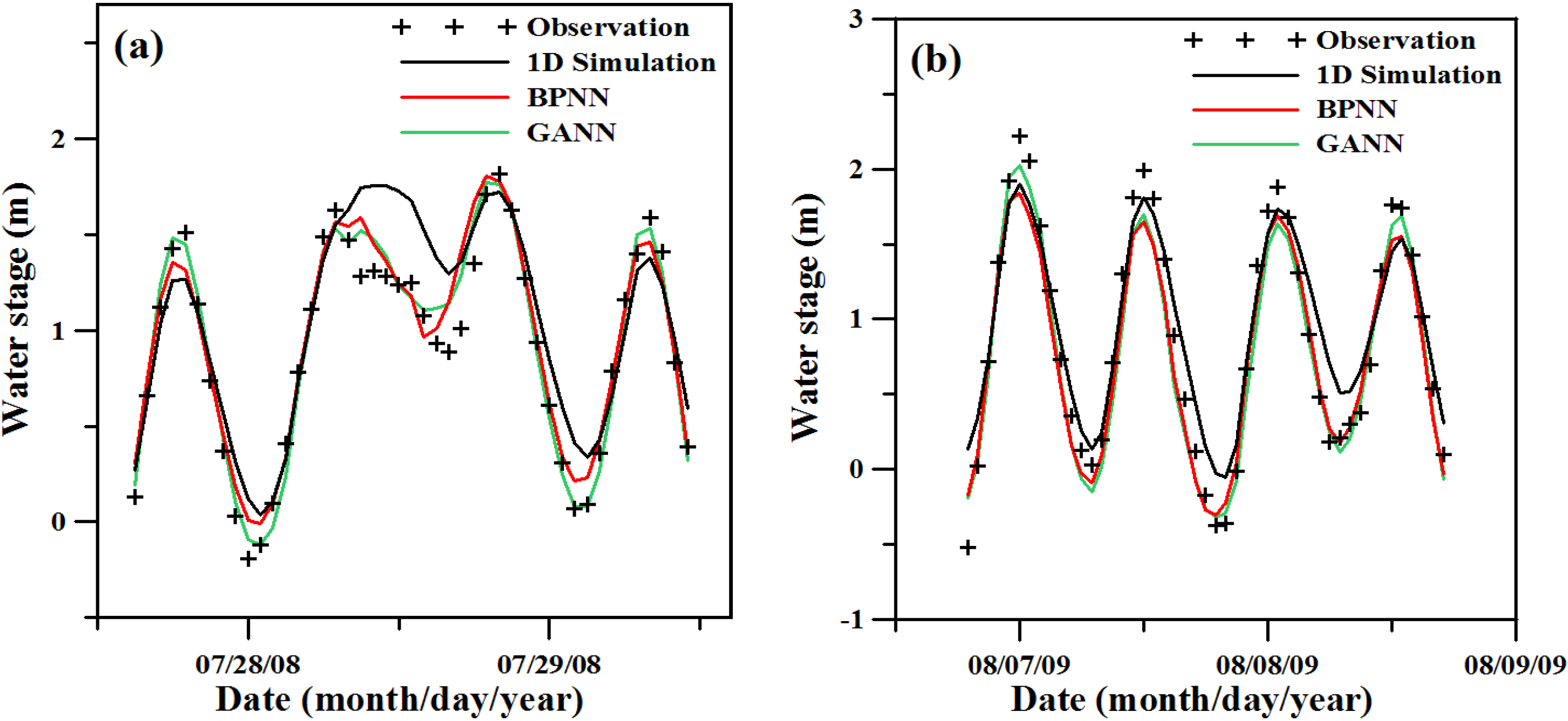
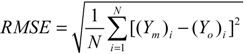
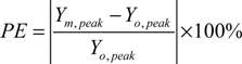
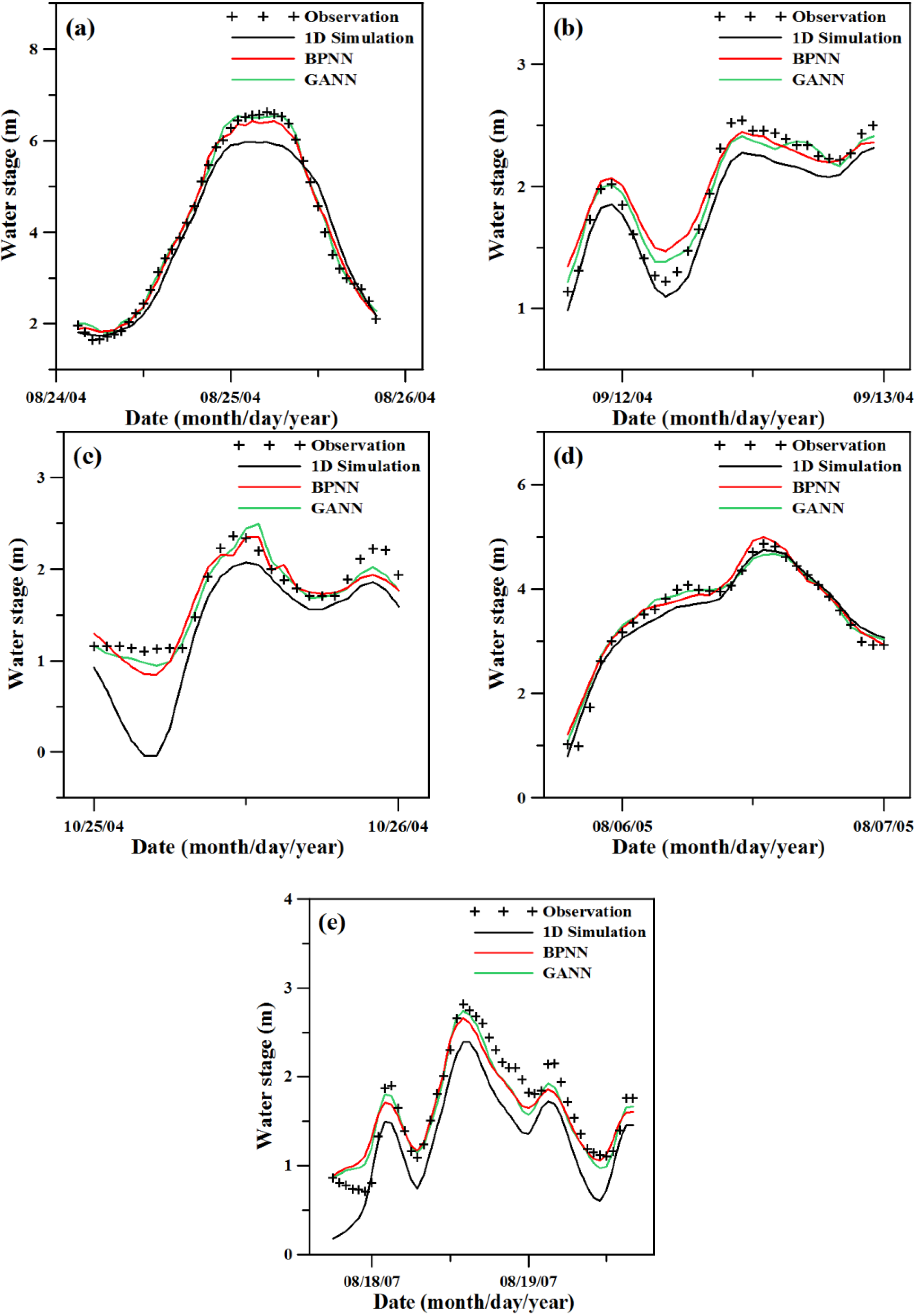
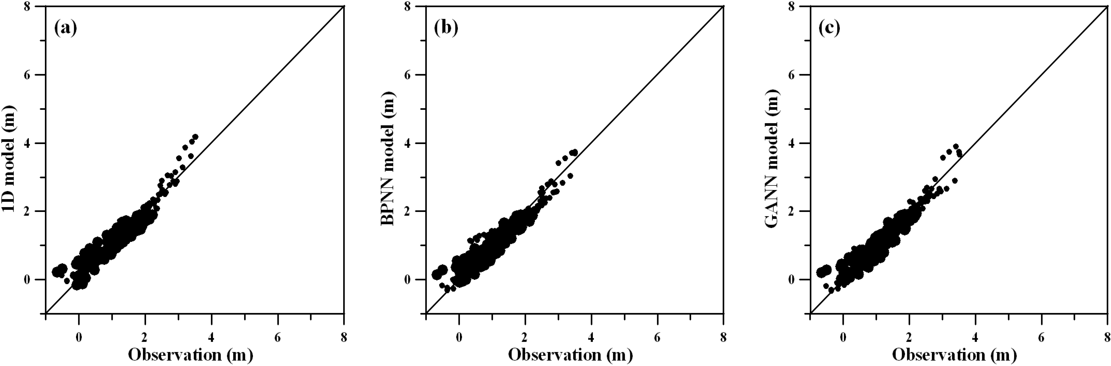
4.2. Flood Routing Hydrodynamic Model Verification and ANN Model Verification

The results in Figure 4 and Table 2 show that the prediction of water stage with the GANN model is better than with either the one-dimensional flood routing hydrodynamic model or the BPNN model. The maximum MAE, RMSE and PE values for the GANN training phase are 0.14 m and 0.19 m, at Chung-Cheng Bridge, and 4.19%, at Ru-Kou-Yan station, respectively. The scatter plot of simulated and observed water stages using the one-dimensional flood routing hydrodynamic model, the BPNN model and the GANN model for five typhoons and four gauge stations is shown in Figure 7. A comparison of the results shows that the GANN technique is successful in predicting the water stage.
The verification results with the one-dimensional flood routing hydrodynamic model for simulating the water stages at Taipei Bridge for Typhoon Fungwong and Typhoon Morakot are shown in Figure 8. Because of space limitations, only the modeling results at Taipei Bridge are shown. The numerical model fails to simulate the water stages during the peak and low tides for these two typhoon events. Table 5 shows the MAE, RMSE and PE for the model validation. The results indicate that the maximum values of MAE, RMSE and PE are 0.22 m and 0.28 m, at Chung-Cheng Bridge, and 13.12%, at Ru-Kou-Yan station, respectively. The MAE and RMSE values are higher than 0.2 m for these four stations.
Figure 8. A comparison of observed and simulated water stages for the flood routing hydrodynamic model, BPNN and GANN model verification at the Taipei Bridge station for (a) Typhoon Fungwong (2008) and (b) Typhoon Morakot (2009).
Water 06 01642 g008
Table 5. The performance of the one-dimensional flood routing hydrodynamic model, the BPNN model and the GANN model with respect to predicting the water stage during the verification phase at four stations.
MethodTaipei BridgeRu-Kou-YanChung-Cheng BridgeDa-Zhi Bridge
MAE (m)RMSE (m)PE (%)MAE (m)RMSE (m)PE (%)MAE (m)RMSE (m)PE (%)MAE (m)RMSE (m)PE (%)
Verification with one-dimensional hydrodynamic model0.200.2510.810.200.2513.120.220.289.860.220.2711.32
Verification with BPNN model0.130.169.890.180.217.170.190.257.990.210.269.02
Verification with GANN model0.090.156.770.l70.204.920.180.236.910.200.247.95
Notes: MAE, mean solute error; RMSE, root mean square error; PE, peak error.
Figure 8 also shows the predicted water stage at Taipei Bridge by BPNN for the two typhoons. The BPNN model improves the predicted water stages compared with using the flood routing hydrodynamic model. The MAE, RMSE and PE values at Taipei Bridge, Ru-Kou-Yan, Chung-Cheng Bridge and Da-Zhi Bridge with the BPNN model are lower than with the flood routing hydrodynamic model (see Table 5). Table 5 also shows the maximum MAE, RMSE and PE values are 0.21 m and 0.26 m, at the Da-Zhi Bridge, and 9.89%, at the Taipei Bridge, respectively, for the BPNN verification phase.
Figure 9 also displays the prediction of water stage at Taipei Bridge by the GANN model during the verification phase. The simulated water stage with the GANN model is better than with the flood routing hydrodynamic model and the BPNN model. This indicates that the GANN model improves the prediction of water stages even though the model cannot fully mimic the high tide at Taipei Bridge during Typhoon Morakot. The MAE, RMSE and PE values at the Taipei Bridge, Ru-Kou-Yan, Chung-Cheng Bridge and Da-Zhi Bridge obtained with the GANN model are less than those obtained with the flood routing hydrodynamic model and the BPNN model. The maximum MAE, RMSE and PE values are 0.20 m and 0.24 m and 7.95% at Da-Zhi Bridge, respectively, for the GANN verification phase (Table 5). The scatter plot of the simulated and observed water stages using the one-dimensional flood routing hydrodynamic model, the BPNN model and the GANN model for two typhoons and four gauge stations for the verification phase is shown in Figure 9. It shows that the GANN model successfully improves the prediction of the water stage during typhoon events.
Figure 9. The scatter plots of simulated and observed water stages using (a) the one-dimensional flood routing hydrodynamic model; (b) the BPNN model; and (c) the GANN model for the verification phase for two typhoon events and four stations.
Water 06 01642 g009

5. Discussions

According to the performance of different approaches, one-dimensional flood routing hydrodynamic model and the combination of one-dimensional flood routing hydrodynamic model and two ANN models (i.e., BPNN and GANN), the simulation for verification phase using a one-dimensional flood routing hydrodynamic model requires approximately 10 minutes of CPU time on an Intel Core I5 PC, while the BPNN and GANN models require only 1.5 and 2.7 min, respectively. The one-dimensional flood routing hydrodynamic model simulation time is long compared to the BPNN and GANN models. The ANN approach can predict water stages in a river system, but the black box limitations of the ANN model result in a failure to simulate the internal physical processes of a river system. The disadvantages of the ANN approach include the proneness to overfitting and the empirical nature of model development.
The simulation results also revealed that GANN model was superior to the BPNN model for predicting water stages. This is the reason that BPNN is a type of neural network that can effectively solve non-linear problems, but there are some problems for BP neural network in the training phase, such as getting into a local extreme, and convergence is slow. To overcome these problems and improve the reliability of the network, the effort of the genetic algorithm is combined with BPNN to avoid local minima and to achieve global convergence quickly and correctly [53,54].
The simulation of physical processes is of critical importance to flood control and water resource management in a river system. The one-dimensional flood routing hydrodynamic model is a physically-based model that can be used to predict water stages response to high freshwater discharge into the river during typhoon events. For the ANN model, which is a data-driven technique, predictability could be increased by providing a large number of appropriate input-output data sets during the training and verification phases [35,55,56]. In this study, we provide an alternative approach: the combination of the one-dimensional flood routing hydrodynamic model (i.e., physical-based model) and the ANN model (i.e., black box model) to improve the accuracy of water stage predictions along the river.

6. Conclusions

The water stages in the Danshuei River system during typhoon events were simulated using a one-dimensional flood routing hydrodynamic model. The observed freshwater discharges at the upstream boundaries and downstream boundary conditions at the Danshuei River mouth were used to drive the model simulation. Five typhoon events, Typhoon Aere (2004), Typhoon Haima (2004), Typhoon Nockten (2005), Typhoon Matsa (2005) and Typhoon Sepat (2007), were used for model calibration (training). Two typhoon events, Typhoon Fungwong (2008) and Typhoon Morakot (2009), were used for model verification. To determine the performance of the hydrodynamic model, the BPNN model, and the GANN model, three criteria (i.e., mean absolute error, MAE; root-mean-square error, RMSE; and peak error, PE) were employed to evaluate the model results and the observational data.
The results showed that the flood routing hydrodynamic model cannot satisfactorily mimic the water stages during the typhoon events for the model calibration and verification phases. Therefore, two ANN models, including the BPNN model and the GANN model, were adopted to improve the water stage predictions during typhoon events using the flood routing hydrodynamic model. The simulated results indicate that the performance with the BPNN model and the GANN model is better than with the hydrodynamic model alone. Moreover, the GANN model predicts the water stage well and presents low MAE, RMSE and PE values at Taipei Bridge, Ru-Kou-Yan, Chung-Cheng Bridge and Da-Zhi Bridge compared with the simulated results using the one-dimensional hydrodynamic model and the BPNN model. This study shows that the GANN technique can be successfully applied to predict water stages in the Danshuei River system during typhoon events.
In the present study, we focus on the water stage prediction instead of forecast during the typhoon events. In a future study, different lead-time forecasts in the water stage can be developed to assist the local authorities with preventing flooding effects prior to typhoon events. The soft computing techniques, such as the combining fuzzy optimal model with genetic programming [47,57], neural network and genetic programming [24,58], support vector machine [59,60,61] and the particle swarm optimization training algorithm for a neural network [29], can also be developed to improve the prediction of water stages along the river system during typhoon events.

Acknowledgments

This research was conducted with the support of the National Science Council, Taiwan, grant No. 101-2625-M-239-001. This financial support is greatly appreciated. The authors would like to express their appreciation to the 10th River Management Bureau, Water Resources Agency, for providing access to the observational data. The authors would also like to thank two anonymous reviewers for their valuable suggestions and comments.

Author Contributions

Wen-Cheng Liu created ideal, supervised the progress, discussed the results, and wrote paper. Chuan-En Chung executed the models.

Conflicts of Interest

The authors declare no conflict of interest.

References

  1. Hsu, M.H.; Fu, J.C.; Liu, W.C. Flood routing with real-time stage correction method for flash flood forecasting in the Tanshui River, Taiwan. J. Hydrol. 2003, 283, 267–280. [Google Scholar] [CrossRef]
  2. Helmio, T. Unsteady 1D flow model of a river with partly vegetated floodplains—Application to the Rhine River. Environ. Model. Softw. 2005, 20, 361–375. [Google Scholar] [CrossRef]
  3. Tayefi, V.; Lane, S.N.; Hardy, R.J.; Yu, D. A comparison of one- and two-dimensional approaches to modeling flood inundation over complex upland floodplains. Hydrol. Process. 2007, 21, 3190–3202. [Google Scholar] [CrossRef]
  4. Patro, S.; Chatterjee, C.; Singh, R.; Raghuwanshi, N.S. Hydrodynamic modeling of a large flood-prone river system in India with limited data. Hydrol. Process. 2009, 23, 2774–2791. [Google Scholar] [CrossRef]
  5. Liu, W.C.; Chen, W.B.; Hsu, M.H.; Fu, J.C. Dynamic routing modeling for flash flood forecast in river system. Nat. Hazards 2010, 52, 519–537. [Google Scholar] [CrossRef]
  6. Malekmohammadi, B.; Zahraie, B.; Kerachian, R. A real-time operation optimization model for flood management in river-reservoir systems. Nat. Hazards 2010, 53, 459–482. [Google Scholar] [CrossRef]
  7. Costabile, P.; Macchione, F. Analysis of one-dimensional modeling for flood routing in compound channels. Water Resour. Manag. 2012, 26, 1065–1087. [Google Scholar] [CrossRef]
  8. Sanyal, J.; Carbonneua, P.; Densmore, A. Hydraulic routing of extreme floods in a large ungauged river and the estimation of associated uncertainties: A case study of the Damodar River, India. Nat. Hazards 2013, 66, 1153–1177. [Google Scholar] [CrossRef] [Green Version]
  9. Saleh, F.; Ducharne, A.; Flipo, N.; Oudin, L.; Ledoux, E. Impact of river bed morphology on discharge and water levels simulated by a 1D Saint-Venant hydraulic model at regional scale. J. Hydrol. 2013, 476, 169–177. [Google Scholar] [CrossRef]
  10. Basheer, I.A.; Hajmeer, M. Artificial neural networks—Fundamentals, computing, design, and application. J. Microbiol. Meth. 2000, 43, 3–31. [Google Scholar] [CrossRef]
  11. Taromina, R.; Chau, K.W.; Sethi, R. Artificial neural network simulation of hourly groundwater levels in a coastal aquifer system of the Venice lagoon. Eng. Appl. Artif. Intel. 2012, 25, 1670–1676. [Google Scholar] [CrossRef]
  12. Cheng, C.T.; Chau, K.W.; Sun, Y.G.; Lin, J.Y. Long-term prediction of discharges in Manwan Reservoir using neural network models. Lect. Notes Comput. Sci. 2005, 3498, 1040–1045. [Google Scholar] [CrossRef]
  13. Chau, K.W.; Wu, C.L.; Li, Y.S. Comparison of several flood forecasting models in Yangtz River. J. Hydrol. Eng. ASCE 2005, 10, 485–491. [Google Scholar] [CrossRef]
  14. Chen, W.; Chau, K.W. Intelligent manipulation and calibration of parameters for hydrological models. Int. J. Environ. Pollut. 2006, 28, 432–447. [Google Scholar] [CrossRef]
  15. Kisi, O. Streamflow forecasting using different artificial neural network algorithm. J. Hydrol. Eng. ASCE 2007, 12, 532–539. [Google Scholar] [CrossRef]
  16. Kisi, O. River flow forecasting and estimation using different artificial neural network techniques. Hydrol. Res. 2008, 39, 27–40. [Google Scholar] [CrossRef]
  17. Pramanik, N.; Panda, R.K. Application of neural network and adaptive neuro-fuzzy inference systems for river flow prediction. Hydrol. Sci. J. 2009, 54, 247–260. [Google Scholar] [CrossRef]
  18. Mukerji, A.; Chatterjee, C.; Raghuwanshi, N.S. Flood forecasting using ANN, neuro-fuzzy, and neuro-GA models. J. Hydrol. Eng. ASCE 2009, 14, 647–652. [Google Scholar] [CrossRef]
  19. Wu, C.L.; Chau, K.W. Predicting monthly streamflow using data-driven models coupled with data-preprocessing techniques. Water Resour. Res. 2009, 45, W08432. [Google Scholar]
  20. Talei, A.; Chua, L.H.C.; Wong, T.S.W. Evaluation of rainfall and discharges inputs used by Adaptive Network-based Fuzzy Inference Systems (ANFIS) in rainfall-runoff modeling. J. Hydrol. 2010, 391, 248–262. [Google Scholar] [CrossRef]
  21. Machado, F.; Mine, M.; Kaviski, E.; Fill, H. Monthly rainfall-runoff modelling using artificial neural networks. Hydrol. Sci. J. 2011, 56, 349–361. [Google Scholar] [CrossRef]
  22. Toukourou, M.; Johannet, A.; Dreyfus, G.; Ayral, P.A. Rainfall-runoff modeling of flash floods in the absence of rainfall forecasts: The case of “Cevenol flash floods”. Appl. Intell. 2011, 35, 178–189. [Google Scholar] [CrossRef]
  23. Wu, C.L.; Chau, K.W. Rainfall-runoff modeling using artificial neural network coupled with singular spectrum analysis. J. Hydrol. 2011, 399, 394–409. [Google Scholar] [CrossRef]
  24. Kisi, O.; Shiri, J.; Mustafa, T. Modeling rainfall-runoff process using soft computing techniques. Comput. Geosci. 2012, 51, 108–117. [Google Scholar] [CrossRef]
  25. Sattari, M.T.; Apaydin, H.; Ozturk, F. Flow estimations for the Sohu Stream using artificial neural networks. Environ. Earth Sci. 2012, 66, 2031–2045. [Google Scholar] [CrossRef]
  26. De Vos, N.J. Echo state networks as an alternative to traditional artificial neural networks in rainfall-runoff modelling. Hydrol. Earth Syst. Sci. 2013, 17, 253–267. [Google Scholar] [CrossRef] [Green Version]
  27. Rezaeianzadeh, M.; Tabari, H.; Yazdi, A.A.; Isik, S.; Kalin, L. Flood flow forecasting using ANN, ANFIS and regression models. Neural. Comput. Applic. 2013. [Google Scholar] [CrossRef]
  28. Alvisi, S.; Mascellani, G.; Franchini, M.; Bardossy, A. Water level forecasting through fuzzy logic and artificial neural network approach. Hydrol. Earth Syst. Sci. 2006, 10, 1–17. [Google Scholar] [CrossRef]
  29. Chau, K.W. Particle swarm optimization training algorithm for ANNs in stage prediction of Shing Mun River. J. Hydrol. 2006, 329, 363–367. [Google Scholar] [CrossRef]
  30. Bustami, R.; Bessaih, N.; Bong, C.; Suhaili, S. Artificial neural network for precipitation and water level predictions of Bedup River. IAENG Int. J. Comput. Sci. 2007, 34, 228–233. [Google Scholar]
  31. Sulaiman, M.; El-Shafie, A.; Karim, O.; Basri, H. Improved water level forecasting performance by using optimal steepness coefficients in an artificial neural network. Water Resour. Manag. 2011, 25, 2525–2541. [Google Scholar] [CrossRef]
  32. Nguyen, P.K.T.; Chua, L.H.C.; Son, L.H. Flood forecasting in large rivers with data-driven models. Nat. Hazards 2014, 71, 767–784. [Google Scholar] [CrossRef]
  33. Moeini, M.H.; Etemad-Shahidi, A.; Chegini, V.; Rahmani, I. Wave data assimilation using a hybrid approach in the Persian Gulf. Ocean. Dynam. 2012, 62, 785–797. [Google Scholar] [CrossRef]
  34. Demirel, M.C.; Venancio, A.; Kahya, E. Flow forecast by SWAT model and ANN in Pracana basin, Portugal. Adv. Eng. Softw. 2009, 40, 467–473. [Google Scholar] [CrossRef]
  35. Panda, R.K.; Pramanik, N.; Bala, B. Simulation of river stage using artificial network and MIKE 11 hydrodynamic model. Comput. Geosci. 2010, 36, 735–745. [Google Scholar] [CrossRef]
  36. Chen, W.B.; Liu, W.C.; Hsu, M.H. Comparison of ANN approach with 2D and 3D hydrodynamic models for simulating estuary water stage. Adv. Eng. Softw. 2012, 45, 69–79. [Google Scholar] [CrossRef]
  37. Liu, W.C.; Chen, W.B.; Hsu, M.H. The influence of discharge reductions on salt water intrusion and residual circulation in Danshuei River. J. Mar. Sci. Technol. 2011, 19, 596–606. [Google Scholar]
  38. Hsu, M.H.; Kuo, A.Y.; Kuo, J.T.; Liu, W.C. Procedure to calibrate and verify numerical models of estuarine hydrodynamics. J. Hydraul. Eng. ASCE 1999, 125, 166–182. [Google Scholar] [CrossRef]
  39. Preissman, A. Propagation of Translatory Waves in Channels and Rivers. In Proceedings of the First Congress of French Association for Computation, Grenoble, France, 1961; pp. 433–442.
  40. Amein, M.; Fang, C.S. Implicit flood routing in natural channel. J. Hydraul. Div. ASCE 1970, 96, 2481–2500. [Google Scholar]
  41. Hsu, M.H.; Fu, J.C.; Liu, W.C. Dynamic routing model with real-time roughness updating for flood forecasting. J. Hydraul. Eng. ASCE 2006, 132, 605–619. [Google Scholar] [CrossRef]
  42. Rumelhart, D.E.; Hinton, G.E.; Williams, R.J. Learning representations by back-propagating errors. Nature 1986, 323, 533–536. [Google Scholar] [CrossRef]
  43. Zadeh, R.M.; Amin, S.; Khalili, D.; Singh, V.P. Daily outflow prediction by multi layer perceptron with logistic sigmoid and tangent sigmoid activation functions. Water Resour. Manag. 2010, 24, 2673–2688. [Google Scholar] [CrossRef]
  44. Yonaba, H.; Anctil, F.; Fortin, V. Comparing sigmoid transfer functions for neural network multistep ahead streamflow forecasting. J. Hydrol. Eng. ASCE 2010, 15, 275–283. [Google Scholar] [CrossRef]
  45. Hagan, M.T.; Menhaj, M. Training feedforward networks with the Marquardt algorithm. IEEE Trans. Neural Netw. 1994, 5, 989–993. [Google Scholar] [CrossRef]
  46. Zhu, H.; Jiao, L.; Pan, J. Multi-population genetic algorithm for feature selection. Lect. Notes Comput. Sci. 2006, 422, 480–487. [Google Scholar]
  47. Kisi, O.; Cengiz, T.M. Fuzzy genetic approach for estimating reference evapotranspiration of Turkey: Mediterranean region. Water Resour. Manag. 2013, 27, 3541–3553. [Google Scholar] [CrossRef]
  48. Wang, W.C.; Chau, K.W.; Cheng, C.T.; Qiu, L. A comparison of performance of several artificial intelligence methods for predicting monthly discharge time series. J. Hydrol. 2009, 374, 294–306. [Google Scholar] [CrossRef]
  49. Chen, W.B.; Liu, W.C.; Hsu, M.H. Predicting typhoon-induced storm surge tide with a two-dimensional hydrodynamic model and artificial neural network model. Nat. Hazards Earth Syst. Sci. 2012, 12, 3799–3809. [Google Scholar] [CrossRef]
  50. Ghose, D.K.; Panda, S.S.; Swain, P.C. Prediction of water table depth in western region, Oissa using BPNN and RBFN neural networks. J. Hydrol. 2010, 394, 296–304. [Google Scholar] [CrossRef]
  51. Goldberg, D. Genetic Algorithm in Search, Optimization and Machine Learning; Addison-Wesley: Boston, MA, USA, 1989. [Google Scholar]
  52. Mulia, I.E.; Tay, H.; Roopsekhar, K.; Tkalich, P. Hybrid ANN-GA for predicting turbidity and chlorophyll-a concentrations. J. HydroEnviron. Res. 2013, 7, 279–299. [Google Scholar]
  53. Chatterjee, S.; Bandopadhyay, S. Reliability estimation using a genetic algorithm-based artificial neural network: An application to a load-haul-dump machine. Expert. Syst. Appl. 2012, 39, 10943–10951. [Google Scholar] [CrossRef]
  54. Karimi, H.; Yousefi, F. Application of artificial neural network-genetic algorithm (ANN-GA) to correlation of density in nanofluids. Fluid Phase Equilibr. 2012, 336, 79–83. [Google Scholar] [CrossRef]
  55. Singh, K.P.; Basant, A.; Malik, A.; Jain, G. Artificial neural network modeling of the river water quality-A case study. Ecol. Model. 2009, 220, 888–895. [Google Scholar] [CrossRef]
  56. Nourani, V.; Komasi, M.; Alami, M.T. Hybrid wavelet-genetic programming approach to optimize ANN modeling of rainfall-runoff process. J. Hydrol. Eng. ASCE 2012, 17, 724–741. [Google Scholar] [CrossRef]
  57. Cheng, C.T.; Ou, C.P.; Chau, K.W. Combining a fuzzy optimal with a genetic algorithm to solve multiobjective rainfall-runoff model calibration. J. Hydrol. 2002, 268, 72–86. [Google Scholar]
  58. Muttil, N.; Chau, K.W. Neural network and genetic programming for modelling coastal algal blooms. Int. J. Environ. Pollut. 2006, 28, 223–238. [Google Scholar] [CrossRef]
  59. Lin, J.Y.; Cheng, C.T.; Chau, K.W. Using support vector machines for long-term discharge prediction. Hydrol. Sci. J. 2006, 51, 599–612. [Google Scholar] [CrossRef]
  60. Tabari, H.; Kisi, O.; Ezani, A.; Hosseinzadeh, T.P. SVM, ANFIS, regression and climate based models for reference evapotranspiration modeling using limited climate data in a semi-arid highland environment. J. Hydrol. 2012, 444, 78–89. [Google Scholar]
  61. Muttil, N.; Chau, K.W. Machine-learning paradigms for selecting ecologically significant input variables. Eng. Appl. Artif. Intel. 2007, 20, 735–744. [Google Scholar] [CrossRef] [Green Version]

