Article

Regional Calibration of SCS-CN L-THIA Model: Application for Ungauged Basins

1
Department of Environmental Engineering, Andong National University, 1375 Gyeongdong Street, Andong 760-749, Korea
2
Regional Infrastructures Engineering, Kangwon National University, 1 Kangwondaehak Street, Chuncheon 200-701, Korea
3
Department of Agricultural and Biological Engineering, Purdue University, 225 South University Street, West Lafayette 47907-2093, IN, USA
*
Author to whom correspondence should be addressed.
Water 2014, 6(5), 1339-1359; https://doi.org/10.3390/w6051339
Submission received: 11 March 2014 / Revised: 5 May 2014 / Accepted: 7 May 2014 / Published: 14 May 2014

Abstract

:
Estimating surface runoff for ungauged watershed is an important issue. The Soil Conservation Service Curve Number (SCS-CN) method developed from long-term experimental data is widely used to estimate surface runoff from gaged or ungauged watersheds. Many modelers have used the documented SCS-CN parameters without calibration, sometimes resulting in significant errors in estimating surface runoff. Several methods for regionalization of SCS-CN parameters were evaluated. The regionalization methods include: (1) average; (2) land use area weighted average; (3) hydrologic soil group area weighted average; (4) area combined land use and hydrologic soil group weighted average; (5) spatial nearest neighbor; (6) inverse distance weighted average; and (7) global calibration method, and model performance for each method was evaluated with application to 14 watersheds located in Indiana. Eight watersheds were used for calibration and six watersheds for validation. For the validation results, the spatial nearest neighbor method provided the highest average Nash-Sutcliffe (NS) value at 0.58 for six watersheds but it included the lowest NS value and variance of NS values of this method was the highest. The global calibration method provided the second highest average NS value at 0.56 with low variation of NS values. Although the spatial nearest neighbor method provided the highest average NS value, this method was not statistically different than other methods. However, the global calibration method was significantly different than other methods except the spatial nearest neighbor method. Therefore, we conclude that the global calibration method is appropriate to regionalize SCS-CN parameters for ungauged watersheds.

1. Introduction

Watershed modeling is one of the rational, economical, and useful approaches for water quality and quantity management and is widely used in planning, design, management and developing watershed management plans, including those for total maximum daily loads (TMDLs). The advance of computer hardware and software allows model frameworks to become more comprehensive, but also more complex [1]. A complex watershed model is generally characterized by a multitude of parameters [2]. Among the large number of parameters, some parameters can be obtained from measurement, but the measurable parameters sometimes have errors, and other parameters cannot be measured. Complex watershed model accuracy might be jeopardized with inappropriate default values [3]. Therefore, model calibration and validation are often needed, and the model calibration-validation scenario analysis is a traditional modeling approach for gauged watersheds.
One of the challenges for hydrologists is to perform hydrologic analysis for ungauged watersheds [4]. Many researchers have attempted to solve this challenge with various watershed models, and Kim and Kaluarachchi [4] have documented the history of parameter estimation for ungauged watersheds. Early attempts to estimate runoff for ungauged watersheds employed calibrated parameters from nearby gauged watersheds with available streamflow [5,6]. However, it has been reported that model results from ungauged watersheds may have errors when basin characteristics such as geography, land use and soil type, are significantly different than those of gauged watersheds [7,8,9]. Recently, a common approach for estimating runoff for ungauged watersheds employs regionalized parameters generated by regression equations assuming model parameters have significant correlation with basin characteristics [4].
The Soil Conservation Service Curve Number (SCS-CN) method [10] is widely employed in various hydrologic models to simulate surface runoff [3]. Since SCS-CN parameters were developed from long-term experimental data, the SCS-CN method estimates rough approximations of direct runoff because it does not include the effects of evapotranspiration and infiltration on watershed wetness [10,11]. To address this limitation, upper curve number values (CN III) and lower curve number values (CN I) were derived from average curve number values (CN II) for “wet” and “dry” antecedent moisture conditions [12]. Although the SCS-CN method was improved to simulate surface runoff by adjustments for antecedent moisture conditions, the SCS-CN parameters recommended by the USDA-NRCS [13] are highly dependent on field conditions or practices even for the same land use type and soil. Several researchers found that SCS-CN parameters sometimes need to be calibrated for application for direct runoff estimation [14]. Grunwald and Norton [15] reported that the simulation results for uncalibrated SCS-CN parameters underestimated observed surface runoff using the Agricultural Nonpoint Source Pollution (AGNPS), and results for calibrated AGNPS were better than uncalibrated results.
The goal of this project was to demonstrate various regionalization methods including: (1) average; (2) land use area weighted average; (3) hydrologic soil group area weighted average; (4) area combined land use and hydrologic soil group weighted average; (5) spatial nearest neighbor; (6) inverse distance weighted average; and (7) global calibration method using the SCE-UA technique for SCS-CN parameters using the Long-Term Hydrologic Impact Assessment (L-THIA) model for 14 watersheds within Indiana.

2. Background

2.1. Shuffled Complex Evolution Algorithm (SCE-UA)

The Shuffled Complex Evolution (SCE-UA) algorithm, developed in the Department of Hydrology and Water Resources of the University of Arizona, along with Genetic Algorithms (GA) are often used for automated model calibration as a global optimization technique. A number of studies have reported that the SCE-UA algorithm provided better results compared to GA approaches for calibrating watershed models [16,17].The SCE-UA method is based on a synthesis of four concepts including: (i) combination of deterministic and probabilistic approaches; (ii) systematic evolution of a “complex” of points spanning the parameter space in the direction of global improvement; (iii) competitive evolution; and (iv) complex shuffling. These four concepts improve its efficiency, flexibility, and effectiveness [18]. The descriptions of each SCE-UA step and more detailed explanations are provided by Duan et al. [19,20] including: (i) generating samples; (ii) ranking points; (iii) partitioning into complexes; (iv) evolving each complex; (v) shuffle complexes; (vi) checking convergence; and (vii) checking the reduction in the number of complexes. S points are sampled in parameter spaces randomly, criteria are calculated at each s points, and s points are ranked from the worst criteria value to the best criteria. The s points are partitioned into p complexes containing m points in partitioning into complexes. According to the competitive complex evolution, each complex is evaluated. The points are combined in the evolved complexes into a single sample population, the sample population is sorted, and the sample population is shuffled into p complexes. Convergence and the reduction in the number of complexes are checked.

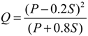
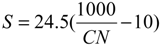
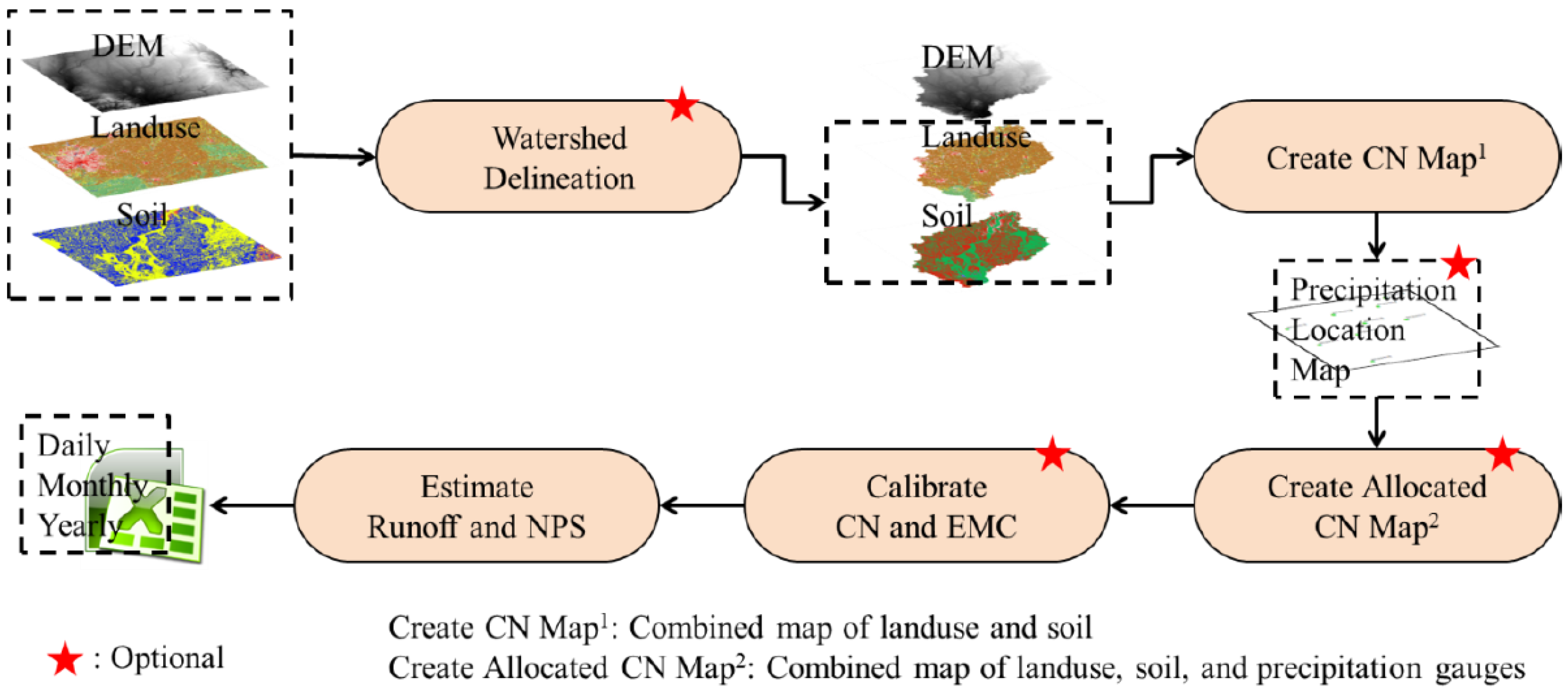
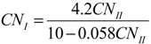
2.2. Overview of L-THIA

L-THIA was developed to evaluate the long-term effects or impacts of land use change on direct runoff and nonpoint source pollution loading [21,22,23,24,25]. Since its introduction, L-THIA has continued to be developed with new L-THIA capabilities being introduced including L-THIA GIS that is integrated with ArcView GIS software and the web-based L-THIA [26]. L-THIA employs the SCS-CN method to estimate direct surface runoff. The SCS-CN method, determined by combination of land use and hydrologic soil group, was developed from observed data by the United States Department of Agriculture, Soil Conservation Service [10] and is widely used for simulating runoff and streamflow [3]. Figure 1 represents the diagram for L-THIA GIS application. The model provides watershed delineation as an option, and creates a SCS-CN map as a GIS grid file using land use and hydrologic soil group maps. From the SCS-CN file and rainfall, the model calculates runoff depth and runoff volume maps using the SCS-CN method. The SCS-CN method is based on a water balance hypothesis that the ratio of actual retention in a watershed to the potential maximum retention is equal to the ratio of actual direct runoff to the potential maximum runoff [10]. Direct surface runoff from the SCS-CN method is expressed by:
Water 06 01339 i001
where, Q is direct surface runoff; P is precipitation; S is potential maximum retention after runoff begins. S is estimated by SCS-CN value as follows:
Water 06 01339 i002
Figure 1. Schematic diagram of Long-Term Hydrologic Impact Assessment (L-THIA) GIS application.
Water 06 01339 g001
Surface runoff is influenced by soil moisture content, and the SCS-CN method was developed to consider antecedent soil moisture condition (AMC) by adjusting SCS-CN value based on seasonal total 5-days rainfall as shown Table 1 [10]. AMC is divided as AMC I for dry condition, AMC II for normal condition, and AMC III for wet condition. SCS-CN values for each AMC I and III are computed from the CN for normal conditions as follows:
Water 06 01339 i003
Water 06 01339 i004
where, CNI is SCS-CN value for AMC I and CNIII for AMC III.
Table 1. The range of optimized Soil Conservation Service Curve Number (SCS-CN) values in L-THIA model.
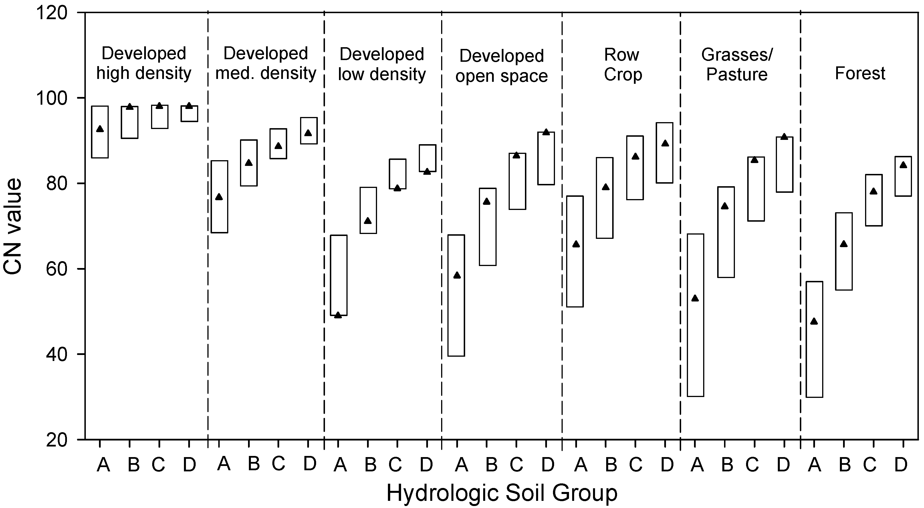
Combination of land use and hydrologic soil groupDocumentedThis study
MinimumMaximumAverageMinimumMaximumMultiplication factor
Developed high density (Impervious area: 80%–100%)A86988985930.97–1.03
B9198949198
C9398969298
D9498979398
Developed medium density (Impervious area: 50%–79%)A68857774800.97–1.03
B7990858188
C8693898693
D8994928895
Developed low density (Impervious area: 20%–49%)A51685149530.96–1.04
B6879747176
C7986827985
D8489868390
Developed open spacesA39685449580.92–1.08
B6179706476
C7486807486
D8089857891
Cultivated cropsA51776459690.92–1.08
B6786777083
C7691847790
D8094878094
Pasture and GrassesA30684945530.92–1.08
B5879696374
C7186797285
D7889847790
ForestA30574440470.92–1.08
B5573645969
C7082767082
D7786827588

3. Materials and Methods

Eight watersheds within Indiana were selected to regionalize SCS-CN method parameters and six watersheds within Indiana were used to validate for applicability of regionalized parameters as ungauged watersheds. The SCE-UA optimization method was developed by coding the SCE-UA version 2.2 developed in the Department of Hydrology and Water Resources of the University of Arizona [19] to fit the L-THIA model because it is widely used to optimize hydrologic models. SCS-CN values and total 5-day rainfall for antecedent moisture condition (AMC) adjustment were optimized through calibration. To maintain the relationship between SCS-CN values for a given land use and hydrologic soil groups, multiple factors for each land use type were obtained as optimized parameters. Therefore, calibrated SCS-CN values were obtained by multiplying the optimized factors and default SCS-CN values for each land use. The optimized range was identified from documented values [10] to avoid searching extreme SCS-CN values and to insure that calibrated SCS-CN values were within reasonable ranges. For the urban area including industrial, commercial, residential, and developed open space, the relationship between percentage impervious area and SCS-CN values was developed using documented values [10] because land use data for urban area was divided by percentage ranges of impervious area. The equations for each hydrologic soil group follow:
CNA = 0.586 × Pimp + 39.116    (R2 = 1.0, n = 9)
CNB = 0.374 × Pimp + 60.666    (R2 = 1.0, n = 9)
CNC = 0.238 × Pimp + 74.070    (R2 = 1.0, n = 9)
CND = 0.175 × Pimp + 80.402    (R2 = 1.0, n = 9)
Therefore, SCS-CN ranges for urban areas were set using Equation (5) and the impervious range for developed high, medium, low density area. The optimized SCS-CN values and multiple factor ranges used in this study are shown in Table 1.
The total 5-day rainfall is typically used to identify soil moisture condition which shifts the soil from one AMC value to another, and the amount often varies with season of the year [27]. The total 5-day rainfall for AMC adjustment was optimized directly within two times for default values, and Table 2 shows the default seasonal 5-day accumulated rainfall for the AMC adjustment [10]. In this study, starting date of growing and dormant seasons was set as 15 April and 15 October, respectively.
Table 2. Default total 5-day antecedent rainfall for antecedent soil moisture condition (AMC) adjustment.
AMCTotal 5-day antecedent rainfall (mm)
Dormant SeasonGrowing Season
ILess than 12.70Less than 35.56
II12.70–27.9435.56–53.34
IIIOver 27.94Over 53.34

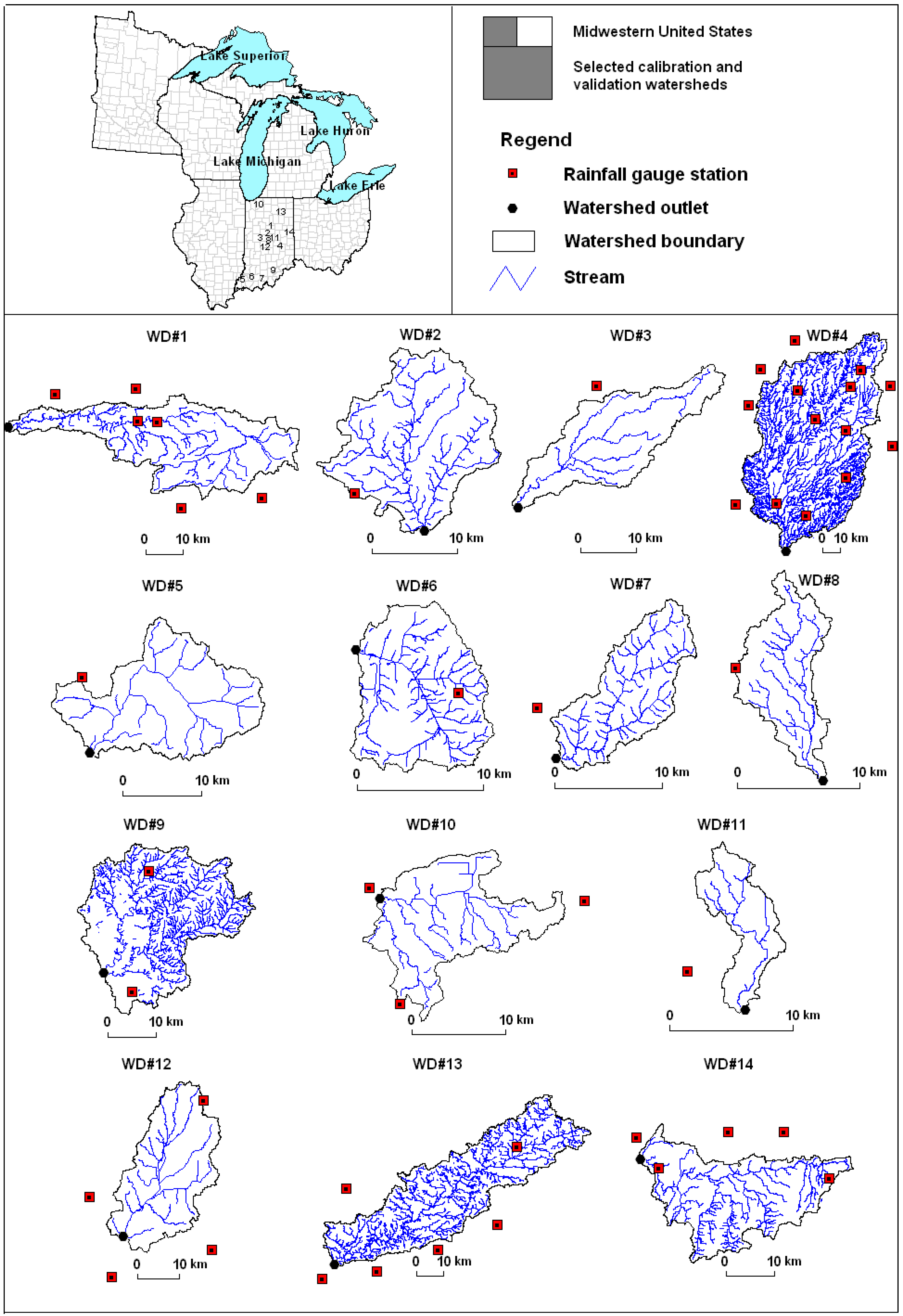
3.1. Study Watersheds and Data

For evaluating the performance of each method for SCS-CN parameter regionalization, eight watersheds for calibration and six watersheds for validation as ungauged watershed were selected based on the absence of lakes or reservoirs in the watershed (Figure 2 and Table 3). Watersheds which included a lake or reservoir were excluded because the observed rainfall-runoff response for these watersheds is typically altered. The selected watershed areas ranged from 32.7 to 5844.1 km2. Calibration watersheds were selected with one or two primary land use types and validation watersheds were selected with mixed urbanized and mixed non-urbanized land uses. Among the calibration watersheds, the primary land use type in the watersheds is crop, with watersheds WD#1 to WD#4 containing 72%–83% crop land use. Pasture and grass areas for the eight calibration watersheds ranged between 1% and 17%. Forest areas were dominant for watersheds WD#6 to WD#7 with 66%–71% forest area. One watershed (WD#8) had urban as the primary land use with about 96% of its area considered urban. Among the six validation watersheds, two watersheds are mixed rural watersheds containing 22% cropped, 35% pastured, and 37% forested area for WD#9 and 26% cropped, 16% pastured, and 42% forested area for WD#10. WD#11 is a mixed urban watershed with 5% high, 12% medium, and 32% low density development, and 39% developed open space. The other watersheds from WD#12 to 14 contain largely cropped areas (71%–73%).
Figure 2. Study watersheds.
Water 06 01339 g002
Table 3. Study Watershed Descriptions.
Watershed (WD)#Watershed nameArea (km2)Calibration periodValidation periodUSGS stationRainfall station
(COOPID)
Land use (%) *Hyd. soil group (%) **
1Wildcat Creek1024.31996–2005 03334000122638, 122931, 124662, 124667, 128784, 129905H: 1, M: 1, L: 4, O: 7, A: 1, B: 52,
C: 80, P: 2, F: 5, W:1C: 47, D: 1
2Eagle Creek268.81996–2005 03353200129557H: 0, M: 0, L: 2, O: 8, A: 0, B: 50,
C: 73, P: 10, F: 6, W:1C: 46, D: 3
3Big Raccoon Creek364.71996–2005 03340800121873H: 0, M: 0, L: 1, O: 5, A: 0, B: 49,
C: 83, P: 5, F: 7, W:0C: 51, D: 1
4East Fork White River5844.11996–2005 03365500121326, 121747, 123527, 123547, 124272, 124642, 124832, 125613, 125923, 126056, 126164, 126437, 127646, 127999H: 0, M: 1, L: 2, O: 6, A: 0, B: 51,
C: 72, P: 5, F: 13, W:1C: 47, D: 2
5Big Creek269.21996–2005 03378550127083H: 0, M: 0, L: 1, O: 7, A: 0, B: 54,
C: 81, P: 1, F: 9, W:0C: 45, D: 1
6South Fork Patoka River110.71999–2004 03376350128442H: 0, M: 0, L: 0, O: 3, A: 0, B: 38,
C: 21, P: 6, F: 66, W:3C: 57, D: 5
7Middle Fork Anderson102.81996–2005 03303300127724H: 0, M: 0, L: 0, O: 4, A: 0, B: 61,
C: 6, P: 17, F: 71, W:1C: 36, D: 3
8Little Eagle Creek70.11996–2005 03353600124249H: 10, M: 20, L: 38, O: 27, A: 0, B: 33,
C: 0, P: 0, F: 4, W:1C: 39, D: 28
9Blue River730.9 1996–200503302800126697, 127755H: 0, M: 0, L: 0, O: 5, A: 0, B: 66,
C: 22, P: 35, F: 37, W: 0C: 34, D: 0
10Little Calument River165.9 1996–200504094000124244, 124837, 128999H: 0, M: 2, L: 6, O: 5, A: 3, B: 57,
C: 26, P: 16, F: 42, W: 3C: 31, D: 9
11Crooked Creek46.6 1996–200503351310124249H: 5, M: 12, L: 32, O: 39, A: 0, B: 54,
C: 4, P: 3, F: 6, W:1C: 45, D: 1
12Deer Creek623.7 1996–200503358000121647, 122041, 125407, 128290H: 0, M: 0, L: 1, O: 5, A: 0, B: 47,
C: 71, P: 9, F: 14, W:0C: 49, D: 3
13Ell River2042.5 1994–200403328500121739, 124181, 125117, 126864, 127482, 129138, 129243H: 0, M: 0, L: 1, O: 6, A: 4, B: 37,
C: 77, P: 5, F: 10, W: 2C: 58, D: 2
14White River568.0 1996–200503347000121229, 122825, 126023, 126164, 127398, 129678H: 0, M: 1, L: 3, O: 7, A: 0, B: 35,
C: 73, P: 6, F: 8, W: 2C: 62, D: 2
Notes: * H is developed high density; M is developed medium density; L is developed low density; O is developed open space; C is crop; P is pasture and grass; F is forest; and W is water; Bold and underline indicates the dominant land use type; ** A means high infiltration (low runoff); B means moderate infiltration (moderate runoff); C means low infiltration (moderate to high runoff); and D means very low infiltration (high runoff); Bold and underlined indicates dominant hydrologic soil group.
The spatial distribution of hydrologic soil groups was obtained from the State Soil Survey Geographic (SSURGO) database obtained from the USDA Natural Resources Conservation Service (USDA-NRCS) website [28]. National Land Cover Data (NLCD 2001) for spatial distribution of land use type was downloaded from the Multi-Resolution Land Characteristics Consortium web site [29]. Land use was divided into eight categories: water, developed high density, developed medium density, developed low density, crop, pasture and grass, forest, and developed open space.
Streamflow must be separated to obtain direct runoff for automatic calibration purposes because the L-THIA model, like many hydrologic models, simulates direct runoff. Recently, digital filtering methods have been widely used for hydrograph separation [30,31,32,33]. Streamflow data were obtained from USGS streamflow gauging stations, and each USGS streamflow gauging station name of the study watersheds is listed in Table 3. The streamflow was separated to obtain direct runoff using the Web-based Hydrograph Analysis Tool (WHAT) with the digital BFLOW filter method [31,33,34].
Daily precipitation data were obtained from the National Climatic Data Center (NCDC) for the 169 stations operated currently within Indiana. Using location information of NCDC stations, Thiessen polygons were generated. Therefore, various precipitation patterns were considered in model application. Weather stations used for each watershed are listed in Table 3.

3.2. L-THIA Application

SCS-CN values for each weather station were generated by overlaying land use, hydrologic soil group layers, and Thiessen layers in GIS grid format using the ArcView 3.3 software [35]. The layer of SCS-CN values was clipped for each study watershed, and input files for L-THIA were generated using the clipped SCS-CN layer. Although the calibration tool for L-THIA was developed to optimize parameters on a daily, monthly, or yearly basis, monthly optimization was adopted because the L-THIA model does not consider routing processes. However, L-THIA simulates runoff on a daily basis. Calibration and validation processes were performed during 1996–2005. Simulation performance was tested by calculating the average error (AE), relative error (RE), root mean square error (RMSE), and Nash-Sutcliffe (NS). The NS coefficient was used as the objective function for optimization. The Nash-Sutcliffe coefficient is commonly used for evaluating hydrological simulation performance. These are defined as follows [36,37,38]:
Water 06 01339 i005
Water 06 01339 i006
Water 06 01339 i007
Water 06 01339 i008
where, Qobs is the observed monthly direct runoff; Qsim is the simulated monthly direct runoff; and Qobs is average monthly observed direct runoff. If the simulated and observed values are the same, AE, RE, and RMSE are 0 and NS is 1.0.

3.3. Baseline Simulations with SWAT Default Values

L-THIA employed the default SCS-CN values from the Soil and Water Assessment Tool (SWAT) and was applied to 14 calibration and validation watersheds for evaluating simulation performance of default SCS-CN values. Because NLCD 2001 land use type for urban area is divided into developed high, medium, and low density, and open space according to the range of impervious area, default SCS-CN values from SWAT were selected considering the default impervious area for each land use type from the SWAT database. The SWAT default SCS-CN values for NLCD 2001 land use type are listed in Table 4.
Table 4. Soil and Water Assessment Tool (SWAT) default SCS-CN value for National Land Cover Data (NLCD) 2001 land use type.
NLCD 2001 land use typeHydrologic soil groupLand use type
ABCD
Developed-high density (80%–100%)87929495Industrial (84%)
Developed-medium density (50%–79%)71828890Residential-high density (60%)
Developed-low density (20%–49%)56748286Residential-medium density (38%)
Developed-open space35627480Residential-low density (12%)
Crop67788589Agricultural Land-Low Crop
Pasture & grass49697984Pasture
Forest35627480Forest-Mixed

3.4. SCS-CN Parameters Regionalization Methods

The process of transferring parameters from neighboring watersheds to the watershed of interest is generally referred to as regionalization [39]. Seven methods were used for regionalizing SCS-CN values: average (method 1), land use area weighted average (method 2), hydrologic soil group area weighted average (method 3), area combined land use and hydrologic soil group weighted average (method 4), spatial nearest neighbor (method 5), inverse distance weighted average (method 6), and global calibration method (method 7).
The method 1 regionalizes SCS-CN values using the arithmetic average of SCS-CN for each land use and soil type and total 5 day rainfall for classifying soil moisture condition. This method assumes the influence of SCS-CN values which represent both minor and major watershed areas is the same on regionalization of CN values. Methods 2–4 which are area weighted average methods including land use, hydrologic soil group, and combination of land use and hydrologic soil group factors assume that calibrated SCS-CN values from major areas are more accurate than those from minor areas. Total 5-day rainfall for AMC adjustment was generated by arithmetic mean because these parameters are not allocated to land use or hydrologic soil group or the combination of both in the SCS-CN method. Regionalized SCS-CN values in methods 2–4 were generated with the following equation:
Water 06 01339 i009
where, CNregion is regionalized SCS-CN value for combination of land use and hydrologic soil group; CNlocal is locally calibrated SCS-CN value for combination of both; %Alocal is area percentage of each calibration watershed for each factor.
Methods 5 and 6 assume that the calibrated SCS-CN values from closer watersheds are more appropriate for ungauged watershed simulation. The regionalized SCS-CN values were directly obtained from the first and second nearest watersheds from the validation watersheds with method 6, and validation results between the first and second nearest watershed were compared. Inverse distance was used for the weighing factor in method 5 because of the assumption of this method. Regionalized SCS-CN values were achieved from the following equation:
Water 06 01339 i010
where, Dwatershed is distance between calibrated and validated watershed centroids.
The global calibration method attempts to obtain the best possible calibration for all calibration sites combined rather than for each site. The SCE-UA optimization method obtains one SCS-CN parameter set for the best fit to the eight calibration watersheds. The global objective function is calculated from individual objective functions for calibration watersheds as follows:
Water 06 01339 i011
where, NSglobal is the global objective function; m is total number of calibration sites; NSind is individual objective function.
Methods 1 and 7 generate one set of SCS-CN parameters for regionalizing Indianan, and other methods generate a different set of SCS-CN parameters for each validated watershed. Methods 2 and 3, which are area weighted methods, generate a spatial interpolation of documented SCS-CN.

4. Results and Discussion

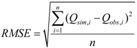
4.1. Baseline Simulation Results for SWAT Default SCS-CN Values

Simulation results for default SCS-CN values in L-THIA are shown in Table 5. The NS values ranged from 0.10 to 0.53. The negative AE and RE values for all watersheds indicate that the runoff results for default SCS-CN values were underestimated compared with observed data. These results indicate that the default SCS-CN values may have potential error for estimating direct runoff , and SCS-CN parameters may need to be calibrated for more accurate simulation.
Table 5. Simulation result for default SCS-CN values.
WD IDNSAERERMSE
WD#10.53−6.27−49.1213.03
WD#20.49−8.15−54.5715.10
WD#30.44−6.82−54.3214.28
WD#40.36−8.74−54.9416.48
WD#50.46−11.22−50.1120.61
WD#60.40−5.53−33.6311.17
WD#70.10−12.76−73.6324.55
WD#80.27−12.55−60.3317.48

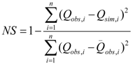
4.2. Calibration Results

The performance of individual watershed calibration shows the calibrated SCS-CN method is able to estimate monthly runoff values well with most watersheds achieving NS values above 0.7 (Table 6). The global calibration method also shows good agreement with NS values above 0.6 but less than the individual watershed calibration results because the global calibration method identified the best model fit for all calibration watersheds rather than for each watershed. The highest NS value was obtained for watershed WD#1 with a NS value of 0.81 for individual calibration and for WD#8 with 0.76 for global calibration. These watersheds are a representative large row crop watershed with 80% of its area in row crops and an urban watershed with 96% of its area in urban, respectively.
Table 6. Individual and global calibration performance of SCS-CN method based on monthly results.
WD IDIndividualGlobalWD IDIndividualGlobal
WD#10.810.60WD#50.740.64
WD#20.760.75WD#60.650.51
WD#30.710.68WD#70.490.38
WD#40.700.67WD#80.790.76

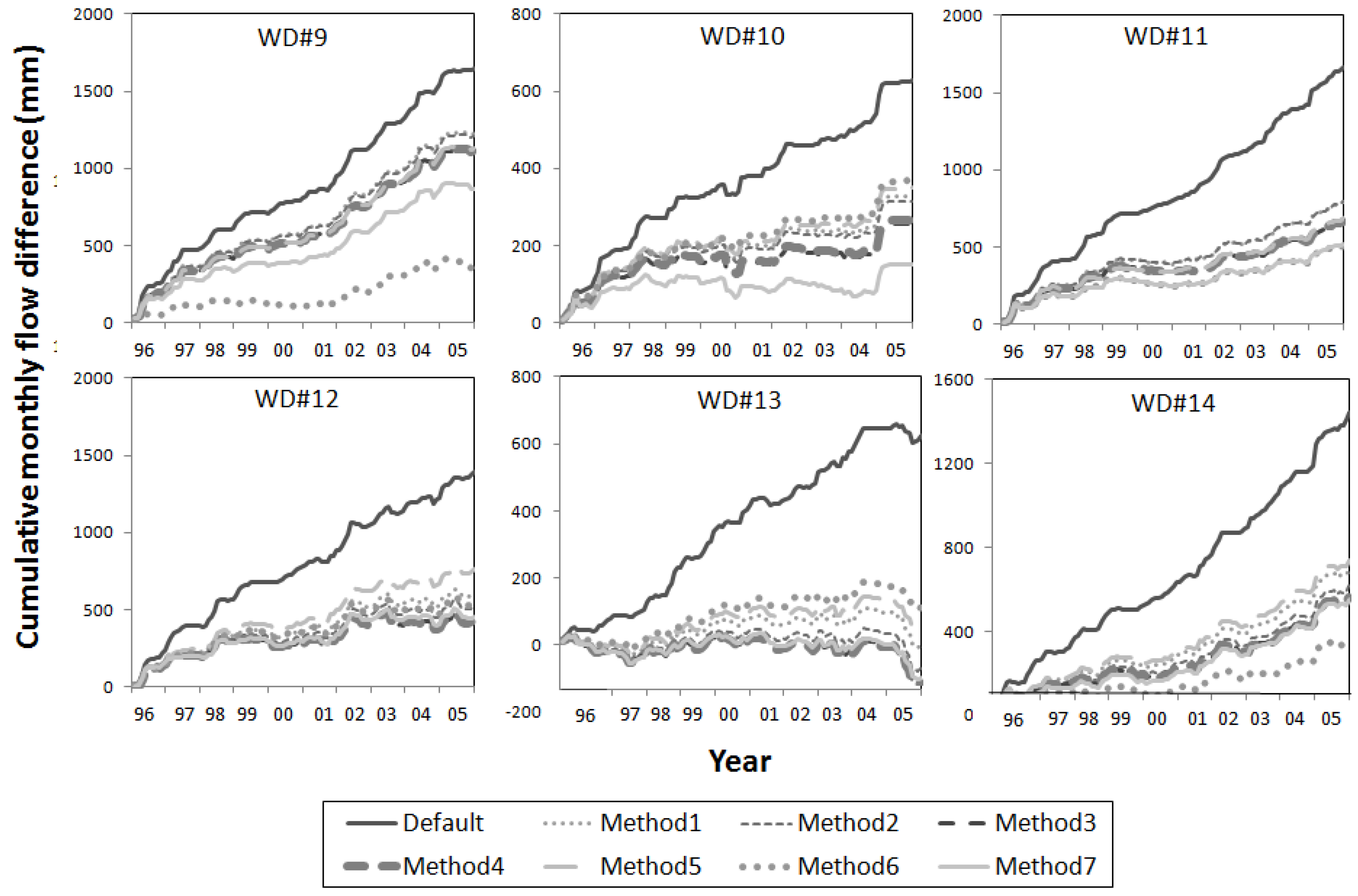
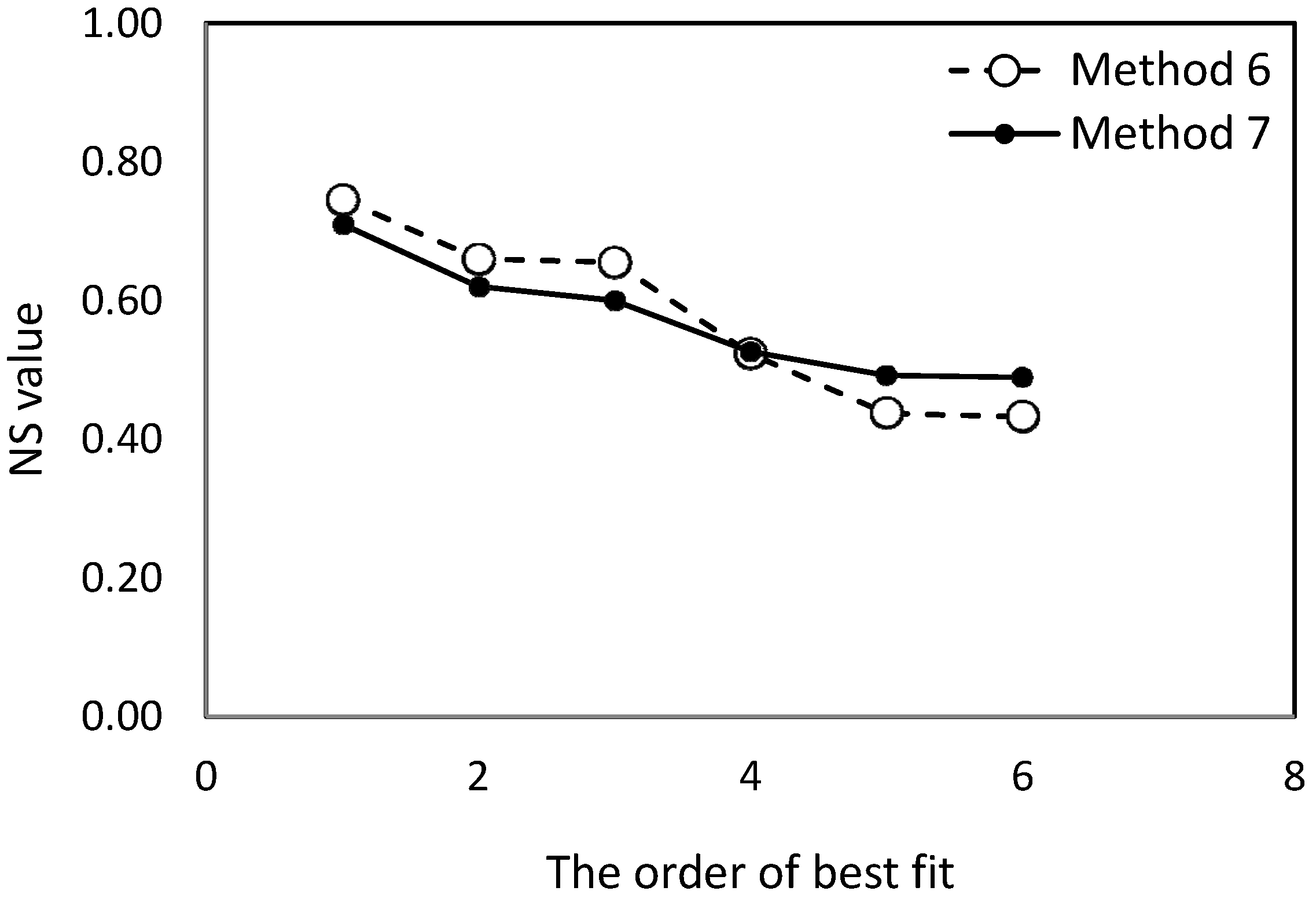
4.3. Comparison of Regionalization Methods

The performance of the regionalization methods on SCS-CN parameters are statistically and graphically shown in Table 7 and Figure 3, respectively. Both methods 1 and 6 provide the poorest runoff simulations compared to other methods with 0.48 average NS value (Table 7). Results for methods 2–4 ranged from 0.48 to 0.50 for average NS values but were not significantly different than results for methods 1 and 6. Method 6 obtained the best runoff simulation with 0.58 average NS value but had high standard deviation, and the global calibration method followed with 0.57 average NS value.
Table 8 shows the statistical analysis of one-paired t-test for NS values of validation watersheds to identify methods statistically different from other methods. All regionalization methods in this study are significantly different from simulation results for default SCS-CN values at an α = 0.01 level. This indicates the methods in this study statistically improve accuracy of runoff simulation for ungauged watersheds. Although method 6 showed the highest NS value for WD#9, among all regionalization methods except the method 7, there were not significant differences with each other. Statistically, method 7 is not significantly different than method 6, but it is significantly different than other regionalization methods at an α = 0.05 level. It indicates that method 7 is statistically more accurate for surface runoff simulation of ungauged watershed than other methods. The scatter plot for observed vs. default and observed vs. method 7 also illustrated the enhancement of simulation performance (Figure 4).
Table 7. Validation performance for regional calibration methods.
MethodsValidation watershed #
#9#10#11#12#13#14MeanSTD
Method 10.430.410.550.460.440.570.480.09
Method 20.430.440.550.480.400.610.480.07
Method 30.490.410.600.470.420.590.500.08
Method 40.490.430.600.480.400.610.500.08
Method 50.490.400.600.440.470.570.480.09
Method 60.750.430.660.490.520.660.580.13
Method 70.600.530.710.560.490.620.570.08
Figure 3. Cumulative monthly flow for validation by regionalizing SCS-CN methods.
Water 06 01339 g003
Methods 2–4 are good methods because the parameters representing greater watershed area are more sensitive within the objective function and can produce more accurate parameters compared to those representing less area, but have a limitation for regionalization of SCS-CN parameters. Although SCS-CN values are well regionalized with the area weighted calculation, regionalization of total 5-day rainfall for AMC adjustment is calculated with an arithmetic average. If there are extraordinary values of these parameters among the calibrated watersheds, sometimes, regionalized total 5-day rainfall for AMC adjustment can be strongly influenced.
Table 8. One paired t-test analysis for regionalization methods.
MethodsArithmetic meanArea weightedDistance weightedNearestGlobal calibration
Land useSoilBoth
Default0.001 *0.001 *0.001 *0.001 *0.001 *0.001 *0.001 *
Method 1 0.5070.1670.1460.3030.0930.008 *
Method 2 0.4820.2330.7350.1410.022 **
Method 3 0.4560.7970.1050.003 *
Method 4 0.6590.1430.009 *
Method 5 0.0740.045 *
Method 6 0.935
Method 7
Notes: * Significant at α = 0.01 level; ** Significant at α = 0.05 level.
Figure 4. 1:1 Scatter plot of the simulated results by default, global calibrated parameters.
Water 06 01339 g004
Method 6 is a widely used approach for simulation of ungauged watersheds. In this study, it is one of the methods which provided the highest and lowest NS values for WD#12 and WD#13, respectively (Table 7). Among the six validation watersheds, in three cases method 6 (WD#9, 13, and 14) obtained higher NS values than method 7. Among these three cases, one case for WD#14 is adjacent to calibration for watershed WD#4. However, method 6 for WD#10 which is the greatest distance for method 6 had the most different NS value with method 7. Figure 4 shows graphically the order of best fit NS values for methods 6 and 7 of six validated watersheds. One of the strengths of method 6 is characteristics of the calibration watershed might be similar with those of an ungauged watershed if the distance between two watersheds is close. However, if the distance is far, sometimes, the similarity of characteristics between two watersheds might differ significantly, and calibrated parameters are improper for simulation of the ungauged watershed. These characteristics of method 6 illustrate high variance of NS values in Figure 5 and Table 7.
Figure 5. Comparison of validated Nash-Sutcliffe (NS) values by the best fit order between methods 6 and 7.
Water 06 01339 g005
In this study, statistical and graphical results support that method 7 is the best way for regionalizing SCS-CN parameters among the methods in this study. High average NS values for method 7 illustrate that this method can well simulate surface runoff for ungauged watershed (Table 7). This was the only method for which the results were statistically different than other methods (Table 8). The validation NS values for method 7 also imply that simulation results for this method are more accurate, moderate and stable than other methods (Figure 5). A major advantage of this method is that the regionalized parameter is optimized by the response of the objective function calculated for all calibration watersheds.

4.4. Regionalized SCS-CN Parameters for Indiana

Regionalized SCS-CN parameters obtained from method 7 and land use characteristics are illustrated in Table 9 and Figure 6. The developed high density, medium density, low density, and open space in this study have the characteristics of “impervious area (paved parking lots, roofs, and driveways, etc.)”, “residential districts with 65% impervious area (average 1/8 acre or less lot size; town house)”, “residential districts with 25% impervious area (average 1/2 acre lot size)”, and “open space (lawns, parks, golf course, cemeteries, etc.) with poor condition (grass cover < 50%)”, respectively [10].
The row crop area in this study area has hydrologic characteristics for “row crops with straight row treatment and good hydraulic condition which is including density and canopy of vegetative area, amount of year-round cover, amount of grass or close-seeded legumes, percent of residue cover on the land surface (poor ≤ 20%), and degree of surface roughness” [10]. The pasture/grass land use represents the characteristics of “the continuous forage for grazing with less than 50% ground cover or heavily grazed with no mulch” [10]. The characteristics of forest in this study were similar to “Forest litter, small trees, and brush are destroyed by heavy grazing or regular burning” [10].
Table 9. Regionalized SCS-CN parameters from global calibration method.
Cover description and AMC conditionCalibrated parametersHydrologic characteristics
SCS-CN ValueDeveloped high densityA:93 B:98 C:98 D:98Impervious area: paved parking lots, roofs, and driveways
Developed medium densityA:80 B:88 C:93 D:96Industrial—75% of impervious area
Developed low densityA:51 B:73 C:81 D:85Residential—average lot size: 1/3 acre
Developed open spaceA:50 B:64 C:74 D:78Grass cover—good condition (> 75%)
CropA:66 B:79 C:86 D:89Row crops with straight row and crop residue cover, and poor hydrologic condition
Pasture/GrassA:53 B:75 C:85 D:91Continuous forage for grazing—poor *
WoodA:48 B:66 C:78 D:84Wood—poor **
Total
5-day rainfall
(mm)
AMCILess than 0.08Dormant season
AMC II0.08–0.69
AMC IIIOver 0.69
AMCILess than 17.12Growing season
AMC II17.12–53.16
AMC IIIOver 53.16
Notes: * Less than 50% ground cover or heavily grazed with no mulch; ** Forest litter, small trees, and brush are destroyed by heavy grazing or regular burning.
Figure 6. Regionalized SCS-CN value for combination of land use and hydrologic soil group from global calibration method.
Water 06 01339 g006
Regionalized total 5-day rainfall for AMC adjustment also illustrated that hydrologic condition of calibrated watersheds is poor so we can assumed that infiltration is impaired and runoff tends to increase. During the growing season, soil moisture condition shifts from dry to moderate condition with 17.2 mm for total 5-day rainfall (Table 8). Soil moisture condition of watersheds indicated wet conditions during the dormant season. Indiana is located at north part of USA and snow pack and frozen soil might occur. Especially, high surface runoff during snow melt might occur and significantly influence optimizing total 5-day rainfall for AMC adjustment during the dormant season. Ficklin and Zhang [40] compared the daily surface runoff of a highly agricultural watershed with uncalibrated SCS-CN and Green-Ampt models and reported the SCS-CN model is slightly better than the Green-Ampt model. However, default SCS-CN parameters from SWAT resulted in simulated results that are significantly lower than the observed surface direct runoff in Indiana as shown in Figure 4. Although SCS-CN parameters were regionalized by method 7, yearly validation results were still slightly underestimated (Figure 4). Therefore, the applicability of the uncalibrated SCS-CN model needs to be evaluated for various watershed conditions. Grimaldi et al. [41] reported most net rainfall intensity values used in the SCS-CN method are underestimated for small watersheds in Texas, USA, because Ia is constant during the event so it is not related to the infiltration properties of the soil. This may be one reason why the simulated direct runoff by the SCS-CN method is underestimated.
The SCS-CN method has been widely used to estimate surface runoff during several decades and extended to hydrologic models for generating hydrographs. However, the SCS-CN method can have significantly large errors in simulating stream flow using hydrologic models and in hourly or sub-hourly temporal resolution of the net rainstorm hyetograph due to the misconception of the SCS-CN method [42,43]. The SCS-CN method as an infiltration model has significant errors in simulating peak discharge predictions [40]. Some researchers reported the SCS-CN method has a tendency to underestimate the net rainfall at the beginning of the storm and overestimate it at the end [44,45]. In this study, the methods of regionalizing SCS-CN values for application to ungauged basins were evaluated for Indiana USA. However, when using regionalized SCS-CN values, the modeler should use these carefully, fully understanding the approach and limitations.

5. Conclusions

Selection of SCS-CN values for ungauged watersheds to simulate surface runoff is a challenge. Seven regionalization methods for estimating SCS-CN values were investigated: (1) average; (2) land use area weighted average; (3) hydrologic soil group area weighted average; (4) area combined land use and hydrologic soil group weighted average; (5) spatial nearest neighbor; (6) inverse distance weighted average; and (7) global calibration. They were applied and evaluated with application in 14 watersheds. Eight watersheds were used to calibrate SCS-CN values and six watersheds were used to validate values. All the regionalization method results were statistically different than results for default SCS-CN values, indicating that calibration of SCS-CN values was needed to obtain accurate simulation results. The spatial nearest neighbor method provided the highest NS value of 0.58. However, the six NS values for spatial nearest neighbor method included the highest and lowest NS values obtained compared to NS values of other methods. The variance of NS values for the spatial nearest neighbor method is also the highest compared to those of other methods. The results of this method are not statistically different than other methods at the α = 0.05 level. We can conclude that the spatial nearest neighbor method could generate good results for estimating runoff from ungauged watersheds when watershed characteristics of gauged and ungauged watersheds are similar but might have potential errors when characteristics are significantly different. The average NS value for six ungauged watersheds with the global calibration method provided the second highest NS of 0.56 with smaller standard deviation. As a result of statistical analyses, the results from the global calibration method were significantly different than results for other methods at α = 0.05, except for those for the spatial nearest neighbor method. Therefore, the global calibration method is recommended for generating regionalized SCS-CN parameters for simulation of runoff from ungauged watersheds and regionalized SCS-CN parameters through this study could be used in Indiana as regionalized SCS-CN values.

Author Contributions

Ji-Hong Jeon wrote paper, developed L-THIA linked with SCE-UA and applied model. Kyoung Jae Lim reviewed and commented on the model and application. Bernard A. Engel revised paper, recommended and directed this research.

Conflicts of Interests

The authors declare no conflict of interest.

References

  1. Chapra, S.C. Surface Water-Quality Modeling; McGraw-Hill: New York, NY, USA, 1997. [Google Scholar]
  2. Eckhardt, K.; Arnold, J.G. Automatic calibration of distributed catchment model. J. Hydrol. 2001, 251, 103–109. [Google Scholar] [CrossRef]
  3. Shoemaker, L.; Lahlou, M.; Bryer, M.; Kumar, D.; Kratt, K. Compendium of Tools for Watershed Assessment and TMDL Development; EPA-841-B-97-006; USEPA Office of Water: Washington, DC, USA, 1997.
  4. Kim, U.; Kaluarachchi, J.J. Application of parameter estimation and regionalization methodologies to ungauged basins of the Upper Blue Nile River Basin, Ethiopia. J. Hydol. 2008, 362, 39–56. [Google Scholar] [CrossRef]
  5. Mosley, M.P. Delimitation of New Zealand hydrologic regions. J. Hydrol. 1981, 49, 173–192. [Google Scholar] [CrossRef]
  6. Vandewiele, G.L.; Elias, A. Monthly water balance of ungauged catchments obtained by geographical regionalization. J. Hydrol. 1995, 170, 277–291. [Google Scholar] [CrossRef]
  7. Post, D.A.; Jones, J.A.; Grant, G.E. An improved methodology for predicting the daily hydrologic response of ungauged catchments. Environ. Model. Softw. 1998, 13, 395–403. [Google Scholar] [CrossRef]
  8. Beven, K.J.; Freer, J.; Schulz, K. The use of generalized likelihood measures for uncertainty estimation in higher-order models of environmental systems. In Nonlinear and Nonstaionary Signal Processing; Fizgerald, W.J., Smith, R.C., Walden, A.T., Young, P.C., Eds.; Cambridge University Press: Cambridge, UK, 2000. [Google Scholar]
  9. Wagener, T.; Wheater, H.S. Parameter estimation and regionalization for continuous rainfall-runoff models including uncertainty. J. Hydrol. 2006, 320, 132–154. [Google Scholar] [CrossRef]
  10. United States Department of Agriculture, Soil Conservation Service (USDA-SCS). National Engineering Handbook Hydrology Chapters: Chapter 10 Estimation of Direct Runoff from Storm Rainfall; USDA-SCS: Washington, DC, USA, 2004.
  11. United States Department of Agriculture, Soil Conservation Service (USDA-SCS). A Method for Estimating Volume and Rate of Runoff in Small Watersheds; Tech. Paper 149; USDA-SCS: Washington, DC, USA, 1973.
  12. Young, D.F.; Carleton, J.N. Implementation of a probabilistic curve number method in the PRZM runoff model. Environ. Model. Softw. 2006, 21, 1172–1179. [Google Scholar] [CrossRef]
  13. United States Department of Agriculture, Natural Resources Conservation Service (USDA-NRCS). Urban Hydrology for Small Watersheds; Technical Release 55, USDA-NRCS, 210-VI-TR-55; USDA-NRCS: Washington, DC, USA, 1986.
  14. Mohammed, H.; Yohannes, F.; Zeleke, G. Validation of agricultural non-point source (AGNPS) pollution model in Kori watershed, South Wollo, Ethiopia. Int. J. Appl. Earth Obs. Geoinf. 2004, 6, 97–109. [Google Scholar] [CrossRef]
  15. Grunwald, S.; Norton, L.D. Calibration and validation of a non-point source pollution model. Agric. Water Manag. 2000, 45, 17–39. [Google Scholar] [CrossRef]
  16. Cooper, V.A.; Nguyen, V.T.V.; Nicell, J.A. Evaluation of global optimization methods for conceptual rainfall-runoff model calibration. Water Sci. Technol. 1997, 36, 53–60. [Google Scholar] [CrossRef]
  17. Kuczera, G. Efficient subspace probabilistic parameter optimization for catchment models. Water Resour. Res. 1997, 33, 177–185. [Google Scholar] [CrossRef]
  18. Duan, Q.; Sorooshian, S.; Gupta, V.K. Optimal use of the SCE-UA global optimization method for calibrating watershed models. J. Hydrol. 1994, 158, 1015–1031. [Google Scholar]
  19. Duan, Q.; Sorooshian, S.; Gupta, V.K. Effective and efficient global optimization for conceptual rainall-runoff models. Water Resour. Res. 1992, 28, 1015–1031. [Google Scholar] [CrossRef]
  20. Duan, Q.; Gupta, V.K.; Sorooshian, S. A shuffled complex evolution approach for effective and efficient global minimization. J. Optim. Theory Appl. 1993, 76, 501–521. [Google Scholar] [CrossRef]
  21. Grove, M.; Harbor, J.; Engel, B.A.; Muthukrishnan, S. Impact of urbanization on surface hydrology, Little Eagle Creek, Indiana, and analysis of L-THIA model sensitivity to data resolution. Phys. Geogr. 2001, 22, 135–153. [Google Scholar]
  22. Kim, Y.; Engel, B.A.; Lim, K.J.; Larson, V.; Duncan, B. Runoff impacts of land-use change in Inidana river lagoon watershed. J. Hydrol. Eng. 2002, 7, 245–251. [Google Scholar] [CrossRef]
  23. Park, Y.S.; Lim, K.J.; Theller, L.; Engel, B.A. L-THIA GIS Manual; Department of Agricultural and Biological Engineering, Purdue University: West Lafayette, IN, USA, 2013. [Google Scholar]
  24. Tang, Z.; Engel, B.A.; Pijanowski, B.C.; Lim, K.L. Forecasting land use change and its environmental impact at a watershed scale. J. Environ. Manag. 2005, 76, 35–45. [Google Scholar] [CrossRef]
  25. Lim, K.J.; Engel, B.A.; Muthukrishnan, S.; Harbor, J. Effect of initial abstraction and urbanization on estimated runoff using CN technology. J. Am. Water Resour. Assoc. 2006, 42, 629–644. [Google Scholar] [CrossRef]
  26. Long Term Hydrologic Impact Analysis (L-THIA). Available online: https://engineering.purdue.edu/~lthia/ (accessed on 11 March 2014).
  27. Mack, M.J. HER-Hydrologic evaluation of runoff; the soil conservation service curve number technique as an interactive computer model. Comput. Geosci. 1995, 21, 929–935. [Google Scholar] [CrossRef]
  28. National Geospatial Center of Excellence. Available online: http://www.nrcs.usda.gov/wps/portal/nrcs/main/national/ngce/ (accessed on 11 March 2014).
  29. Multi-Resolution Land Characteristics Consortium (MRLC). Available online: http://www.mrlc.gov/index.php (accessed on 11 March 2014).
  30. Lyne, V.D.; Hollick, M. Stochastic Time-Variable Rainfall-Runoff Modeling; Hydrology and Water Resources Symposium, Institution of Engineers Australia: Perth, Australia, 1979. [Google Scholar]
  31. Arnold, J.G.; Allen, P.M. Validation of automated methods for estimating baseflow and groundwater recharge from stream flow records. J. Am. Water Resour. Assoc. 1999, 35, 411–424. [Google Scholar] [CrossRef]
  32. Eckhardt, K. How to construct recursive digital filters for baseflow separation. Hydrol. Process. 2005, 19, 507–515. [Google Scholar] [CrossRef]
  33. Lim, K.J.; Engel, B.A.; Tang, Z.; Choi, J.; Kim, K.S.; Muthukrishnan, S.; Tripathy, D. Automated web GIS based hydrograph analysis tool, WHAT. J. Am. Water Resour. Assoc. 2005, 41, 1407–1416. [Google Scholar] [CrossRef]
  34. WHAT: Web-based Hydrograph Analysis Tool. Available online: https://engineering.purdue.edu/~what/ (accessed on 11 March 2014).
  35. Environmental Systems Research Institute (ESRI). What’s New in ArcView 3.1, 3.2, and 3.3; ESRI: Redlands, CA, USA, 2002. [Google Scholar]
  36. Nash, J.E.; Sutcliffe, J.V. River flow forecasting through conceptual model. Part 1: A discussion of principles. J. Hydrol. 1970, 10, 282–290. [Google Scholar] [CrossRef]
  37. Loague, K.; Green, R.E. Statistical and graphical methods for evaluating solute transport models: Overview and application. J. Contam. Hydrol. 1991, 7, 51–73. [Google Scholar] [CrossRef]
  38. Parajka, J.; Merz, R.; Blöschl, G. A comparison of regionalization methods for catchment model parameters. Hydrol. Earth Syst. Sci. 2005, 9, 157–171. [Google Scholar] [CrossRef]
  39. Blöschl, G.; Sivapalan, M. Scale issues in hydrological modeling—A review. Hydrol. Process. 1995, 9, 251–290. [Google Scholar] [CrossRef]
  40. Ficklin, D.L.; Zhang, M. A comparison of the curve number and Green-Ampt models in a agricultural watershed. Trans. ASABE 2013, 56, 61–69. [Google Scholar] [CrossRef]
  41. Grimaldi, S.; Petroselli, A.; Romano, N. Green-Ampt curve-number mixed procedure as an empirical tool for rainfall-runoff modeling in small and ungauged basins. Hydrol. Process. 2013, 27, 1253–1264. [Google Scholar] [CrossRef]
  42. Garen, D.C.; Moore, D.S. Curve number hydrology in water quality modeling: Uses, abuses, and future directions. J. Am. Water Resour. Assoc. 2005, 41, 377–388. [Google Scholar]
  43. Woodward, D.E.; Hoeft, C.C.; Mullem, J.V.; Ward, T.J. Discussion of “Modifications to SCS-CN method for long-term hydrologic simulation” by K. Geetha, S.K. Mishra, T.I. Eldho, A.K. Rastogi, and R.P. Pandey. J. Irrig. Drain Eng. 2010, 136, 444–446. [Google Scholar]
  44. Eli, R.N.; Lamont, S.J. Curve numbers and urban runoff modeling—Application limitations. In Low Impact Development 2010: Redefining Water in the City, Proceedings of the 2010 International Low Impact Development Conference, San Francisco, CA, USA, 11–14 April 2010; pp. 405–418.
  45. Grimaldi, G.; Petroselli, A.; Romano, N. Curve-number/Green-Ampt mixed procedure for streamflow predictions in ungauged basins: Parameter sensitivity analysis. Hydrol. Process. 2013, 27, 1265–1275. [Google Scholar] [CrossRef]

