Article

A New Method for Urban Storm Flood Inundation Simulation with Fine CD-TIN Surface

1
Key Laboratory of Environment Change and Natural Disaster, Beijing Normal University, Beijing 100875, China
2
Internet of Things Perception Mine Research Center, China University of Mining and Technology, Xuzhou 221008, China
3
Beijing Research Center of Urban Systems Engineering, Beike Building, No. 27, West 3rd Ring Rd North, Haidian District, Beijing 100089, China
4
Computer Network Teaching and Information Department, Beijing University of Civil Engineering and Architecture, No.1 Zhanlanguan Road, Beijing 10004, China
5
Institute for Geo-Informatics and Digital Mine Research, Northeastern University, Shenyang 110819, China
*
Author to whom correspondence should be addressed.
Water 2014, 6(5), 1151-1171; https://doi.org/10.3390/w6051151
Submission received: 11 February 2014 / Revised: 5 April 2014 / Accepted: 11 April 2014 / Published: 5 May 2014

Abstract

:
Urban storm inundation, which frequently has dramatic impacts on city safety and social life, is an emergent and difficult issue. Due to the complexity of urban surfaces and the variety of spatial modeling elements, the lack of detailed hydrological data and accurate urban surface models compromise the study and implementation of urban storm inundation simulations. This paper introduces a Constrained Delaunay Triangular Irregular Network (CD-TIN) to model fine urban surfaces (based on detailed ground sampling data) and subsequently employs a depression division method that refers to Fine Constrained Features (FCFs) to construct computational urban water depressions. Storm-runoff yield is placed through mass conservation to calculate the volume of rainfall, runoff and drainage. The water confluences between neighboring depressions are provided when the water level exceeds the outlet of a certain depression. Numerical solutions achieved through a dichotomy are introduced to obtain the water level. Therefore, the continuous inundation process can be divided into different time intervals to obtain a series of inundation scenarios. The main campus of Beijing Normal University (BNU) was used as a case study to simulate the “7.21” storm inundation event to validate the usability and suitability of the proposed methods. In comparing the simulation results with in-situ observations, the proposed method is accurate and effective, with significantly lower drainage data requirements being obtained. The proposed methods will also be useful for urban drainage design and city inundation emergency preparations.

1. Introduction

Urban areas serve as the center of populations, property and resources, and one severe storm flood can result in dramatic property damage and financial losses. In recent years, numerous cities have been inundated by storm floods, which are the major cause of urban flooding. Two thirds of Chinese cities have endured storm inundation, with a portion experiencing more than three storms per year. These severe storms are characterized by maximum water depth greater than 1 meter and inundation durations of longer than 30 min. Urban storm flood inundation has drawn increasing attention in watershed flood research. The proliferation of recent modeling efforts is a direct consequence of significant storm flood events in urban areas and the perceived increased risk from these high rainfall events [1].
Prevailing researches on urban storm flood inundation employ the concept of dual urban drainage system. The urban storm water system is composed of two parts: a surface system and a subsurface system [2,3]. The two parts interact with each other through ponds and overland flow networks to couple the two systems [4,5]. The “1D-1D” approach [6] identifies vertical interactions between the surface and subsurface systems through manholes or groups of water drain grates as a dynamic link between the 1D flow in pipes and 1D flow in surface pathways or canals. In contrast, 1D-2D approaches [7,8,9,10] describe 1D sewer flow integrated with 2D surface flow simulation. Interactions between the two models occur between underground network nodes and surface computational grid cells [11,12]. Some 2D hydraulic models provide the physical process simulation of pluvial flood, such as LISFLOOD [13], LISFLOOD-FP [14]. Furthermore, comparison of 1D/1D and 1D/2D coupled methods is introduced to validate the state-of-art of 1D/2D coupled method [15]. Also, the 1D/2D is employed as the calibration method for 1D/1D in the absence of field data [16]. However, the high quality terrain data and detailed hydrological data (especially drainage system data) required by these methods are difficult to obtain. Moreover, the efficiency of 2D flood modeling is a major challenge [17]. The performance of existing 2D models significantly varies, depending on the choice of time steps and the number of iterations within each time step [18]. In addition, the efficiency of numerical algorithms, the use of multi-processing [19], the hardware specification [20] and other computational overhead costs for modeling must also be considered [21]. These approaches are impractical for real-time representation or rapid simulation of the flooding scenarios [4]. Given the computational and data requirements, another challenge of a ‘‘dual drainage” approach is the paucity of monitoring records of surcharge conditions for model calibration and validation [3,22].
Geographic Information System (GIS) based storm-runoff models that employ a flat-water concept [23,24], can practically handle the above problems to a certain extent. The development of GUFIM [17] provides an option for simulating inundation in some urban areas with an absence of detailed flood hydrology data, high-resolution topographic data and hydraulic overland inundation model. In addition, the time series of storm-runoff modeling results provide flexibility for modeling temporal inundation variations, thus avoiding the time consuming problem of most physically based flood models [25]. However, these methods primarily rely on raster-based urban surfaces. Using a Triangle Irregular Network (TIN) or a Constrained Delauney Triangle Irregular Network (CD-TIN) for representing urban surface has obvious advantages. (1) Constructing a raster from irregularly spaced data or multiple source data often requires interpolation and possible loss of information [26]; (2) Water flow on a grid is commonly constrained to eight (or even four) neighbor directions for ease of computation, which can produce visible artifacts; (3) The extracted flow networks and water depressions may be unrealistic due to the limited regular arrangement of raster fixed cells, such as plume-parallel-shape flow streams and parallel-discrete-shape depressions [27,28]; (4) Different resolution of raster represented terrain can produce different hydrology elements, e.g., flow networks or depressions [29]. The urban water depressions, defined as watershed of the sink point to which water converges, are of importance to serve as basic unit for urban flood simulation. While for actual hydrological modeling, it mainly relies on raster represented terrain in that a regular grid is more amenable for computation. A large number of flow direction assignment [30,31] and depression delineation methods [30,32,33,34] are proposed. However, due to the limitation of raster-based terrain mentioned above, a TIN-based terrain has been used to delineate depression to route the flow path and model the runoff. The runoff networks are generated through analyzing whether the slopes of two adjacent triangles with a common edge forms a ridge, a channel or a plane [26,35]. The flow networks are then calculated along the steepest direction between either the triangle centers or the triangle edges [26,36,37,38]. However, urban surfaces exhibit various small-scale urban features (e.g., curbs, road camber, walls, and buildings, defined as Fine Constrained Features (FCFs) in this paper). The inundation events and the modeling evidence of urban flooding suggest that these small-scale features can have a significant impact on flood propagation [1]. To accurately simulate urban storm flood inundation, these FCFs must be taken into practical consideration.
As a consequence, this research introduces a new method for urban flood inundation simulation. It employs a CD-TIN to represent the fine urban surface, including all types of FCFs (e.g., water drain grates, street curbs, walls, and buildings). As Figure 1 shows, we introduce timely procedures to simulate urban storm inundation. The data acquisition and organization methods are introduced in terms of FCFs through total station, digital level and terrestrial LiDAR. The CD-TIN represented urban surface is built with property of triangular nodes, triangular edges and triangular facets. Urban water depression as the basic unit for flood inundation is generated and its related storm-runoff model, confluence algorithm between depressions are proposed to calculate the inundation depth. The prototype software CityFlood V1.0 is developed and tested. The main campus of Beijing Normal University (BNU) during the “7.21” storm event is studied. Validation and comparison analyses are also introduced.
Figure 1. The flow chart of the proposed method.
Water 06 01151 g001

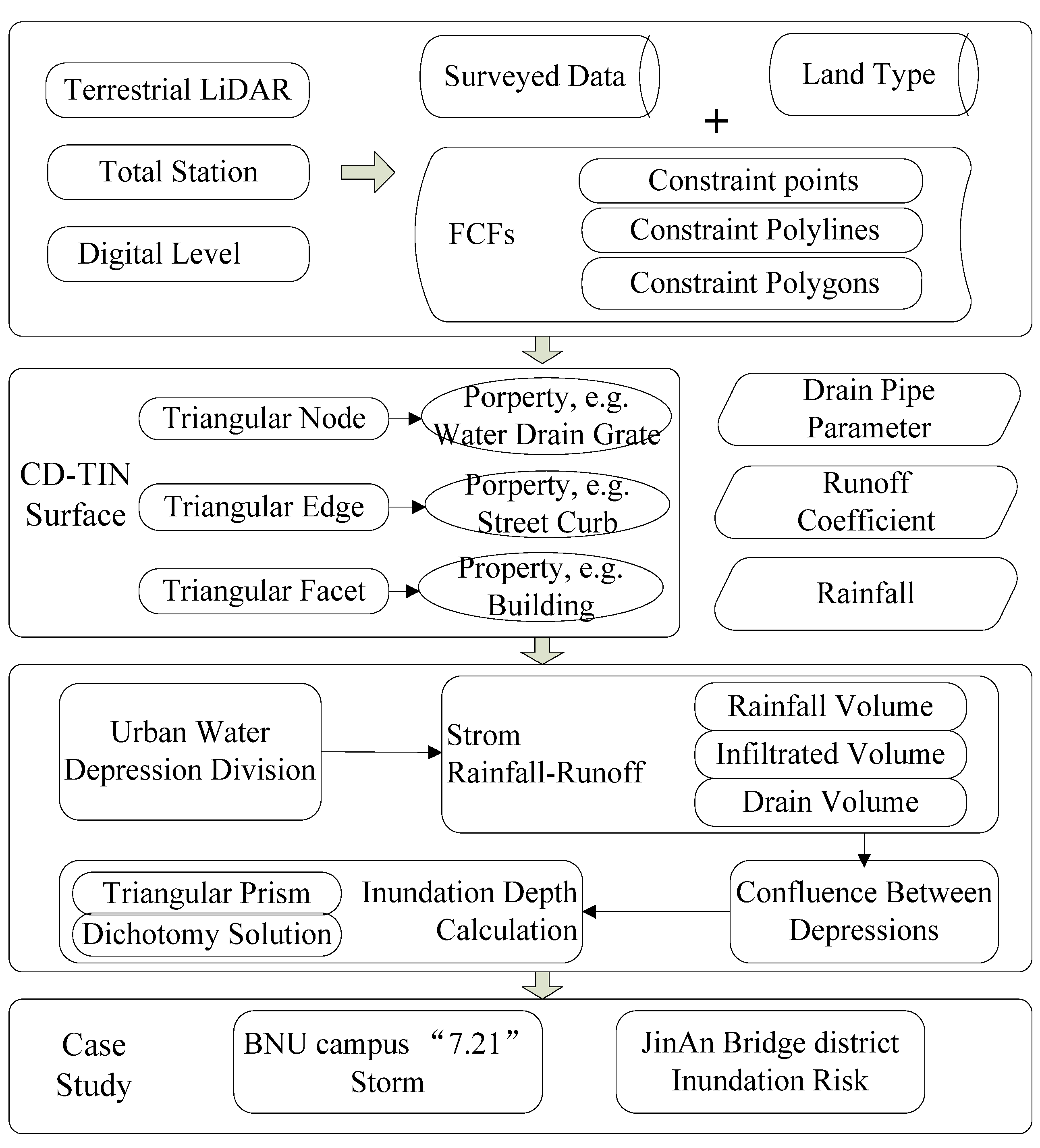
2. Data Acquisition and Urban Surface Modeling

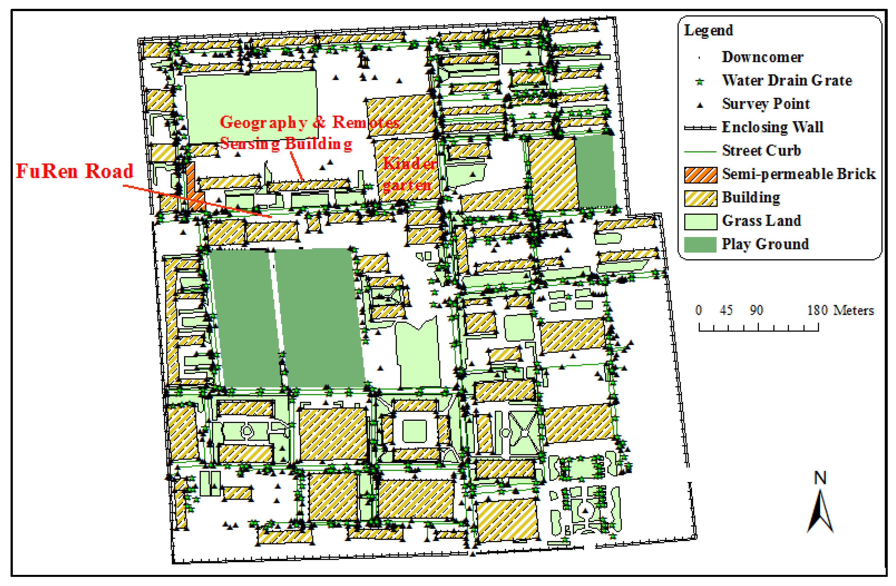
2.1. Data Acquisition and Preprocess

The CD-TIN is an appropriate method for representing the FCFs on an urban surface in detail. Compared with traditional topography which cannot represent these features accurately, a high-resolution DEM acquired from LiDAR data may provide a suitable solution for detailed urban flood modeling [1,39,40]. The terrestrial LiDAR can distinguish the side surfaces of buildings, road cambers and other large urban features, but it has defects to obtain the top surfaces of these urban features. The airborne LiDAR can capture the top surfaces of urban features properly, but some FCFs are often difficult to be distinguished, such as the street curbs, because they may be smaller than the resolution of the measuring instrument (the horizontal accuracy 0.3 m and vertical accuracy 0.15 m). Despite the high cost, raster represented urban surfaces through different interpolate methods can produce different flood inundation results [41]. Due to the high accuracy survey, some political sensitive cities do not permit the airborne LiDAR to survey the urban areas.
Therefore, we utilized total station, digital level and terrestrial LiDAR to survey the urban surface in detail, including all types of FCFs. According to the national grade-IV surveying standard, the surveyed results are of cm precision—sufficiently detailed to represent small scale urban features. Table 1 shows the FCFs stored as Shapefiles (one of the most widely used file formats for ArcGIS) in the form of points (gullies, down comers), polylines (road cambers, walls) or polygons (buildings).
Table 1. Constrained features defined data types and organization.
Constrain FeaturesData TypeData Organization
Water drain grates, Down comers, Outlet of a region, etc.Constrained pointShapefile PointZM
Road cambers, Street curbs, Road isolation strip, Walls, etc.Constrained polylineShapefile PolylineZM
Buildings (or other man-made structures), Grass lands, Playgrounds, Lakes (or other water bodies), etc.Constrained polygonShapefile PolygonZM

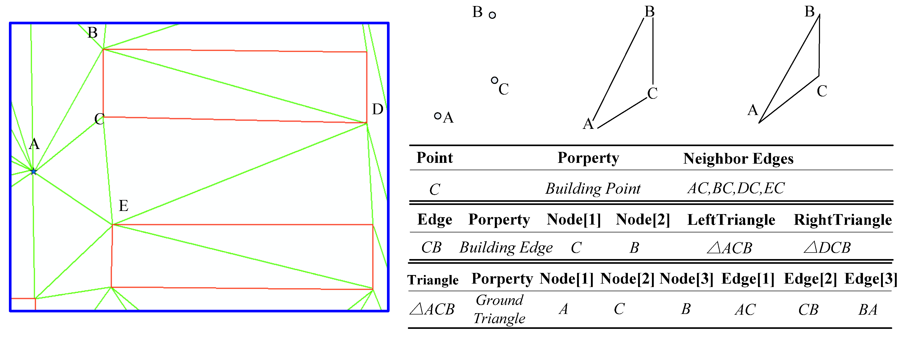
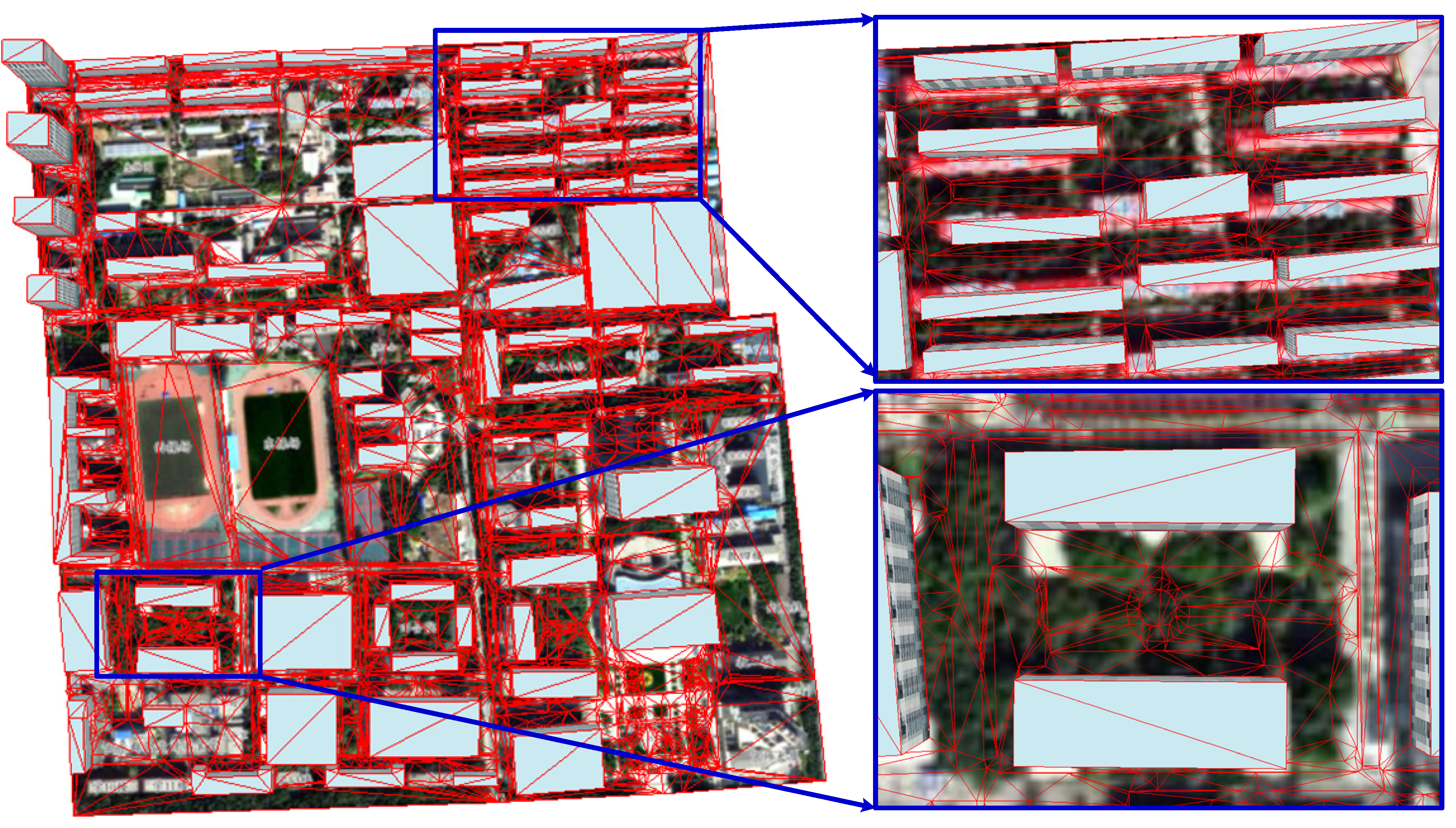
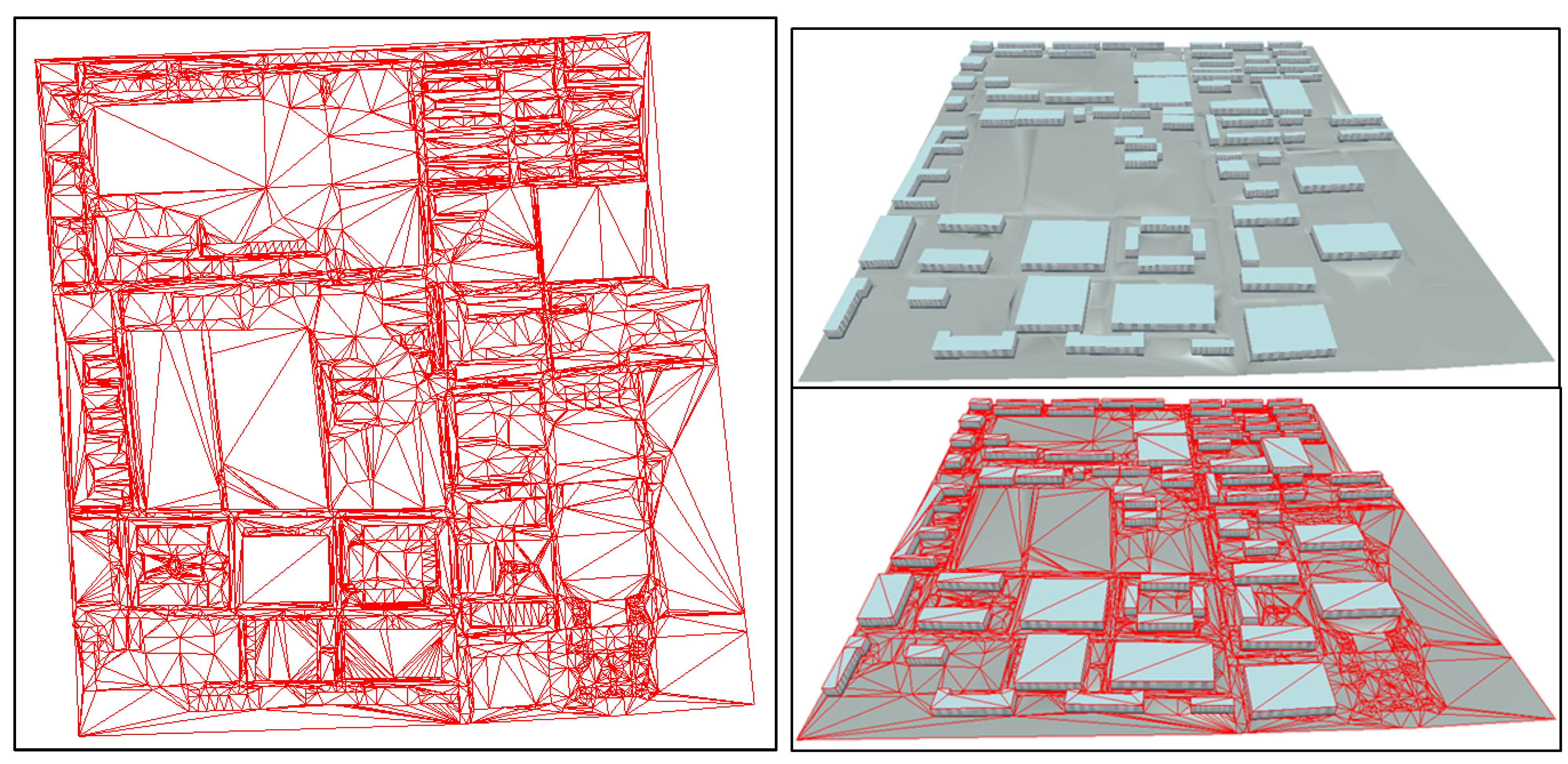
2.2. Modeling Urban Surface with CD-TIN

A CD-TIN representation is introduced to consider the complexity of urban surface and model the detailed FCFs, (illustrated in Table 1; FCFs are shown as red lines in Figure 1). To utilize the surveyed and organized data in Section 2.1, the CD-TIN is generated by employing Bernal and Sloan’s method [42], as shown in Figure 2. The CD-TIN not only considers the shape and boundaries of the FCFs on the urban surface but also records FCFs properties, which can dramatically impact water flow and rainfall-runoff on urban surfaces. For instance, water flow into underground through the point with the property of water drain grate; water flow will change when it encounters a wall or street curb; water runoff volume on a grass land is different than a playground. In Figure 3, we use point A, edge CB, and triangle ACB as examples to record their properties for further analyzing their influence on urban runoff. The topology of the CD-TIN is also recorded for further confluence calculation, including the neighboring edges, the left and right triangles of edge, the nodes and edges of triangle.
Figure 2. Urban surface representation with CD-TIN. The blue stars label the water drain grates; the red lines represent the constrained features such as street curbs, walls, grass lands boundaries and buildings; the green lines represent the normal triangle edges; the blue rectangle labels the detailed illustration area.
Water 06 01151 g002
Figure 3. The illustration of property and topology for CD-TIN in terms of point, edge, and triangle.
Water 06 01151 g003

3. Runoff and Confluence

In the following explanation, several key terminologies related to hydrological analysis are provided as follows: (1) pit point, the local point whose elevation is lower than its neighbour points; (2) watershed, a set of triangles whose trickle paths contain a certain point P; (3) water depression, defined as the watershed of a pit; and (4) outlet, the lowest point among the boundary points of a certain depression.

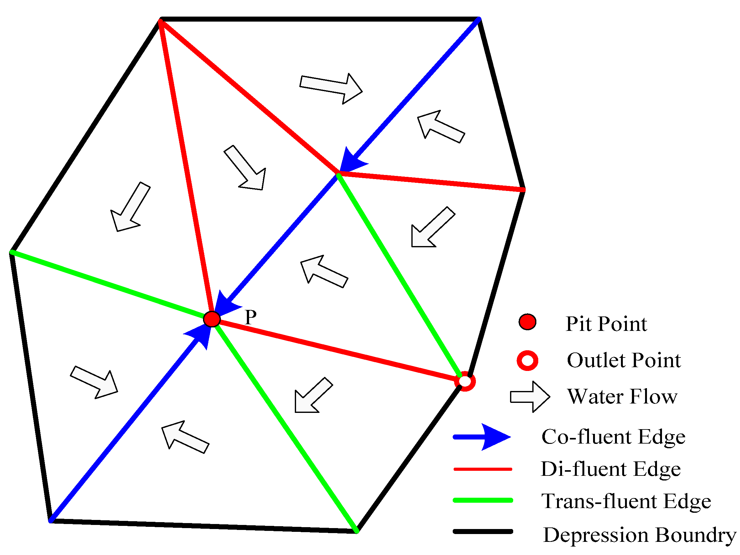
3.1. Computational Urban Water Depression Division

This paper generates a computational urban water depression, which is the basic computational unit to simulate urban storm flood inundation, by employing the facet to edge flow mode [26,43]. We assume that the water on the triangular facet initially flows to its downstream edge, along the steepest direction which is defined as the inverse direction of the gradient on the triangle, subsequently flowing along the downstream edges. With this definition (shown as in Figure 4), we classify the edges into co-fluent, trans-fluent and di-fluent edges referring to their gradients of left and right triangles. The edge properties that influence water runoff are also taken into consideration, such as the building edge being classified as a di-fluent edge. According to the flow relationship of edges in labelling each triangle with different final pit points, the water depression polygon can be generated through these different pit labels, as shown in Figure 5. When the water level of a certain depression exceeds its outlet, the water spills out into its neighboring depressions. The confluence between water depressions is proposed in Section 3.3.
Figure 4. Definition of co-fluent edges, trans-fluent edges, and di-fluent edges. (a) Co-fluent edge is (c| Water on the left and right triangle of edge c where both flow to c); (b) Trans-fluent edge is (t| Water on the left and right triangle of edge t where one flows out from t, and the other flows to t); (c) Di-fluent edge is (d| Water on the left and right triangle of edge d where both flow out from d).
Water 06 01151 g004
Figure 5. Illustration of computational water depression; lines with different colors represent different edge types.
Water 06 01151 g005

3.2. Storm Rainfall Runoff

A flat-water concept [23,24] is an optimal solution for storm runoff calculations, especially for places where hydraulic overland inundation models are not available. The concept relies on the assumption that the surface of the accumulated water is horizontal (gradient h = 0 where h is the elevation of the water surface) [22]. This research adopts the flat-water concept as the inundation basis.
There is an obvious mass balance principle in a certain water depression: the accumulated water Qa is the volume of rainfall excluding water infiltrated into the underground and water conveyed by underground drainage system. Evaporation is not considered in that evaporation can be ignored compared with the accumulated rainfall volume [44]. As shown in Figure 6, the mass balance can be summarized as Equation (1).
Qa = Qy + Qc = (Qf - Qu - Qd) + (Qi - Qo)
where, Qa is the final accumulated water volume (m3); Qy is the accumulated yield water volume (m3); Qc is the accumulated confluence water volume (m); Qf is the rainfall volume during a specified time duration (m3); Qu is the volume of water infiltrated into underground (m3); Qd is the conveyed water volume by underground drainage sewer system (m3); Qi is the water volume flowing in from neighbor depressions (m3); Qo is the water volume flowing out to neighbor depressions (m3).

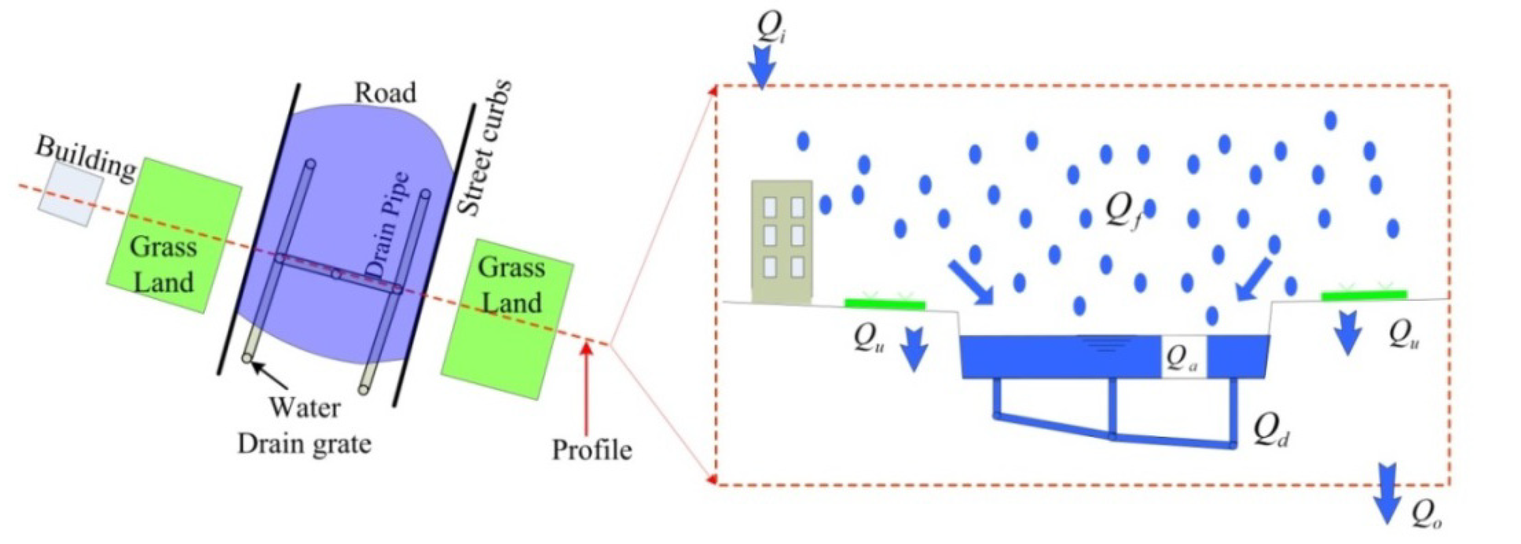
3.2.1. Rainfall Volume Qf

Historic rainfall data is useful data to calculate the accumulative rainfall volume on the condition that all the historic data can be obtained. Otherwise, a design storm can be employed as an option. Based on the relationship of intensity-duration-frequency (IDF), the design storm is defined from a hyetograph to depict the precipitation along the time distribution. In the case study, the IDF equation of a Beijing storm is employed to calculate the rainfall. It is designed by TongJi University through an analytical method [45], shown as Equations (2) and (3). This substitution can calculate the precipitation for the urban area where detailed storm rainfall data are unavailable.
Water 06 01151 i001
Qf = P Sp× 10-3
where P is the precipitation intensity (mm/min); t is the designed rainfall duration t (min); TE is the return frequency (a); Sp is the horizontal projection area of the depression (m2).
Figure 6. The mass balance illustration in a certain computational water depression, the red dashed line represents the profile crossing one road.
Water 06 01151 g006

3.3.2. Infiltrated Volume Qu

A complex urban surface has diverse capacities of infiltration. Previous researches has utilized the time condensation method of hydrograph analysis [46], the detention-flow-relationship method [47], and the most widely used Green-Ampt model [48].These methods primarily focus on the soil ground, while urban surfaces mostly consist of impermeable layers. To easily access and conveniently calculate the parameters, this research employs empirical runoff coefficients to substitute infiltration parameters for calculating the accumulative infiltrated volume (Qc , m3). Equation (1) can then be replaced by Equation (4).
Qa = (Qf - Qc - Qd) + (Qi - Qo)
where Qc = (1 − φ) Qf and φ is the runoff coefficient diversifying with different urban land types; Empirical runoff coefficients can be determined from the Water Supply and Drainage Design Manual [45], as shown in Table 2.
Table 2. The runoff coefficient of different land types.
Land typeRunoff coefficientValue #1Value #2Value #3
Building surface, concrete, or asphalt pavement road0.85~0.950.850.900.95
Large rubble paved road, or gravel road with asphalt surface0.55~0.650.550.600.65
Gradation macadam road0.40~0.500.400.450.50
Masonry brick or gravel road0.35~0.400.350.3750.40
Unpaved soil road0.25~0.350.250.2750.35
Garden or green land0.10~0.200.100.150.20
Water area0000

3.3.3. Drain Volume Qd

Because of data complexity and time consuming computation, also not all the data can be immediately obtained after an urban storm event. In particular, underground sewer system can be very difficult to monitor [22]; therefore, the interactions between surface and subsurface system [4] are outside the scope of this research. We assume that all drainage systems are operating at their full capacity during the storm event. Therefore, the discharge Qd is the designed full capacity of downstream conduit (m3), calculated as [49]:
Water 06 01151 i002
Where δ is the overwhelmed coefficient, which take the value 1 or −1 to label whether the sewer system is overwhelmed; nc is the Manning’s roughness of the conduit; Ad is the full cross-section area of conduit (m2); Rd is the hydraulic radius for full conduit flow (m); and Sd is the friction slope of conduit. The friction slope of conduit Sd can be calculated as Water 06 01151 i005
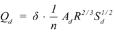
, where h is the elevation difference of original node and end node; l is the length of conduit.
As a consequence, Equation (4) can be replaced by Equation (6) to feasibly compute the accumulative excess water volume feasibly. The simulation duration (T) can be divided into various time slice for inundation simulation scenarios. Thus, Equation (6) can exist at simulation time Ti.
Water 06 01151 i003

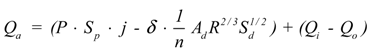
3.3. Confluence between Depressions (Qi, Qo)
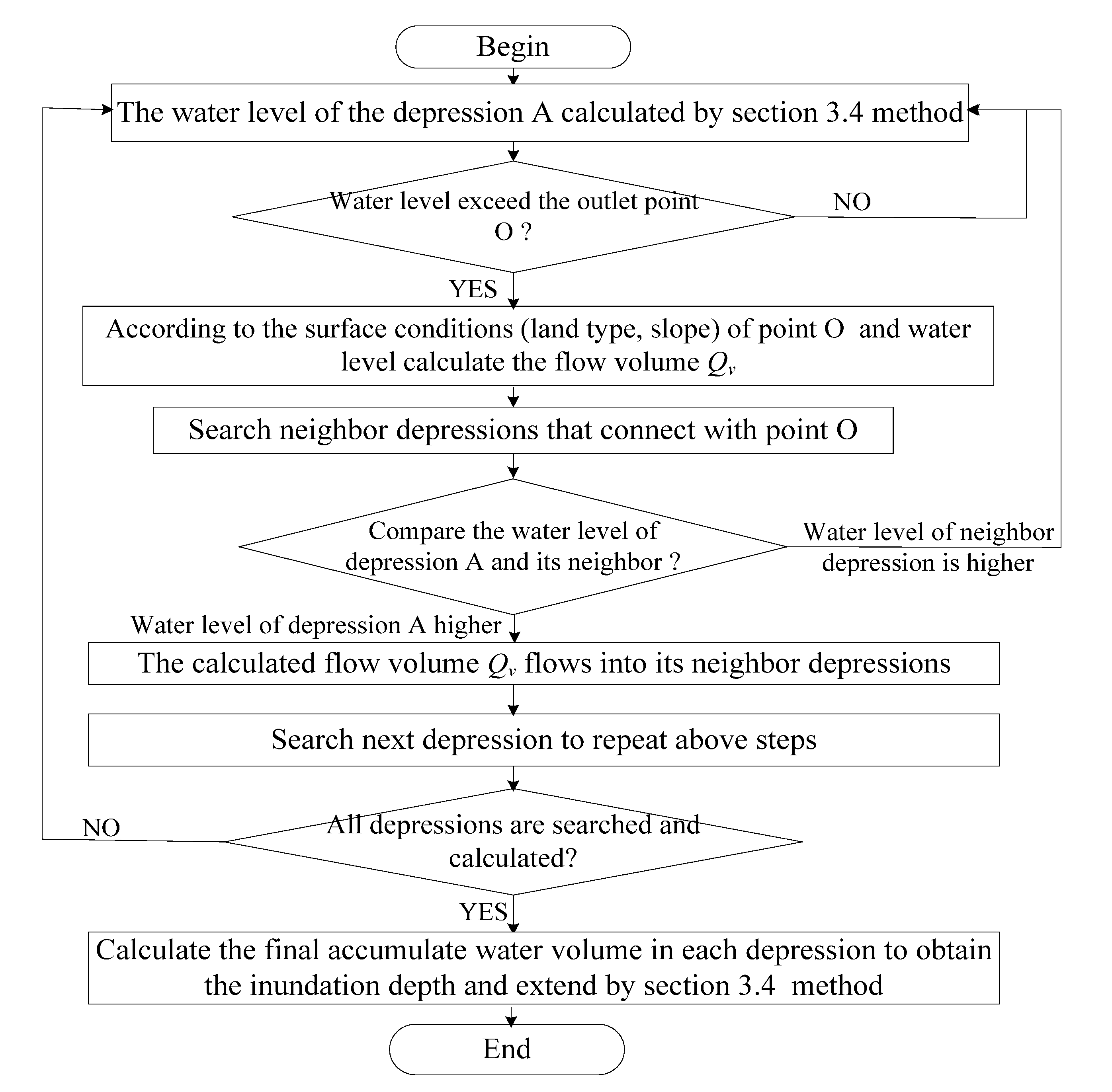
We assume the inundation in each depression complies with the flat-water concept, but it is potential for uneven inundated surfaces between adjacent depressions. Therefore, we propose a novel water confluence between depressions. The flowchart of the algorithm is proposed as shown in Figure 7.
When the accumulated water surface in depression A arrives at the outlet point O, the confluence between depression A and B begins. Taken Figure 8a as an illustration, the detailed confluence procedures are shown as following:
(1)
Judge whether the water level of depression A (Ha) arrive at the outlet point O; If not, Ha continues to rise, else go to step (2);
(2)
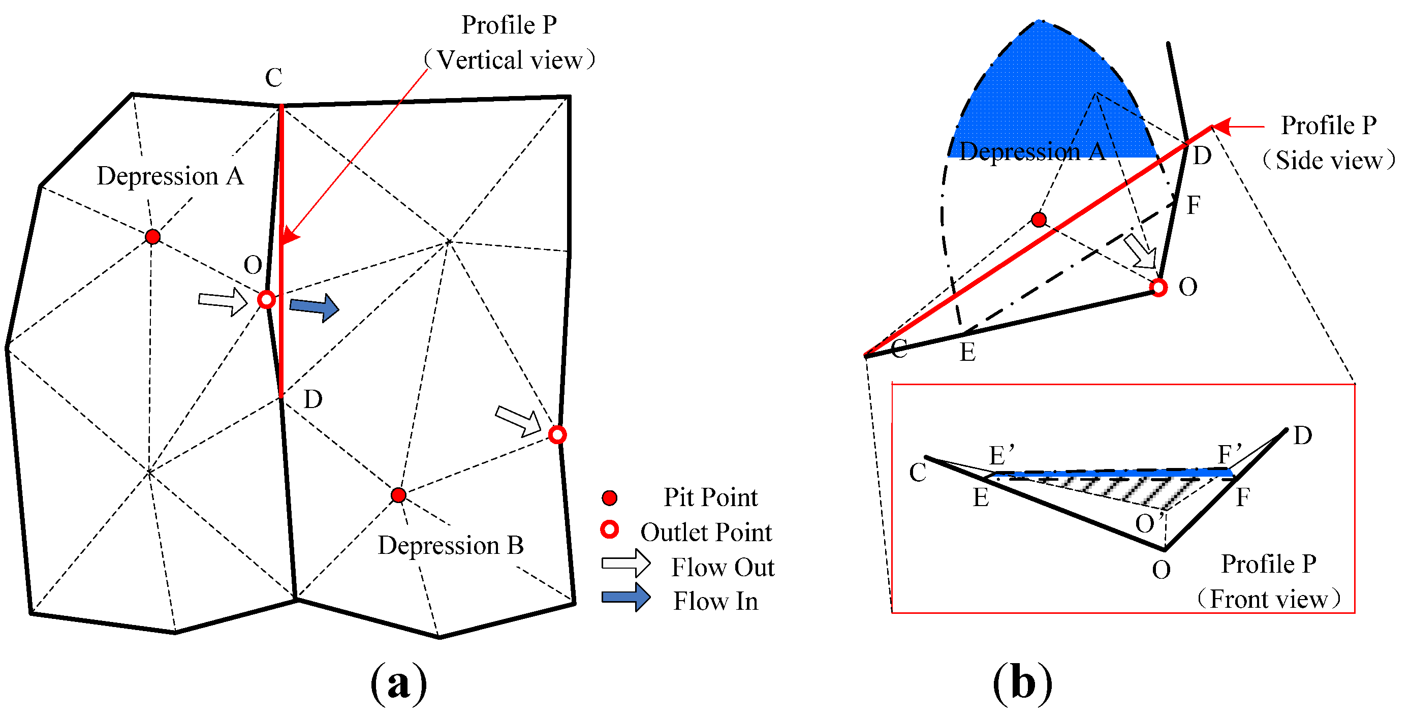
Refer to the conditions of urban surface (land type, slope) and water level; employ empirical Equation (7) [50] to calculate the overland flow water volume Qv:
Water 06 01151 i004
Where, As is the cross section of accumulated water on the outlet point O (m2); k is the constant parameter of overland flow (m/s), which can be obtained from Hao’s research [49]; S is the average slope of the ground. To calculate As, as shown in Figure 8b, we draw the vertical profile P along CD. Then the water surface (blue polygon) insects CO, DO at E and F. Point E, O, F project on P as E’, O’, F’. Thus, As is calculated as the area of △E’O’F’;
(3)
Search the water depressions that connect with O; Judge Ha>Hb, then the accumulated water in depression A flows to depression B at the volume of Qv. Hence, the Qo of depression A is Qv, Qi of depression B is Qv, and vice versa;
(4)
All urban water depressions repeat Steps (1)–(3) to calculate the water confluence which are quantified as the Qi and Qo;
(5)
Calculate the final accumulated water volume in each depression referring to Equation (6).
Figure 7. Algorithm flowchart of confluence between urban water depressions.
Water 06 01151 g007
Figure 8. Confluence mode between neighbor water depressions, red point labels the pit point of the depression; point O is the outlet point of the depression A and depression C; blue polygon represents the water surface. (a) The illustration of water confluence from depression A to depression B; (b) the cross section on the outlet point O.
Water 06 01151 g008

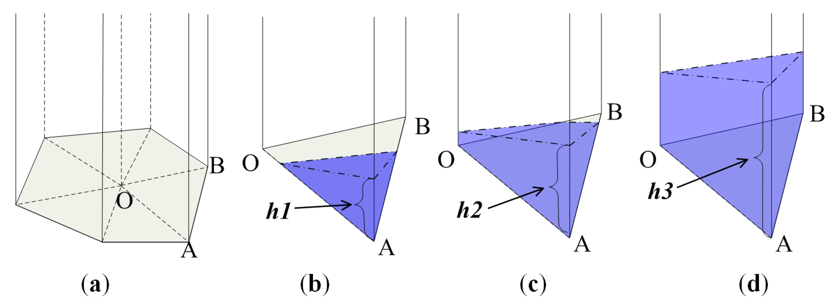
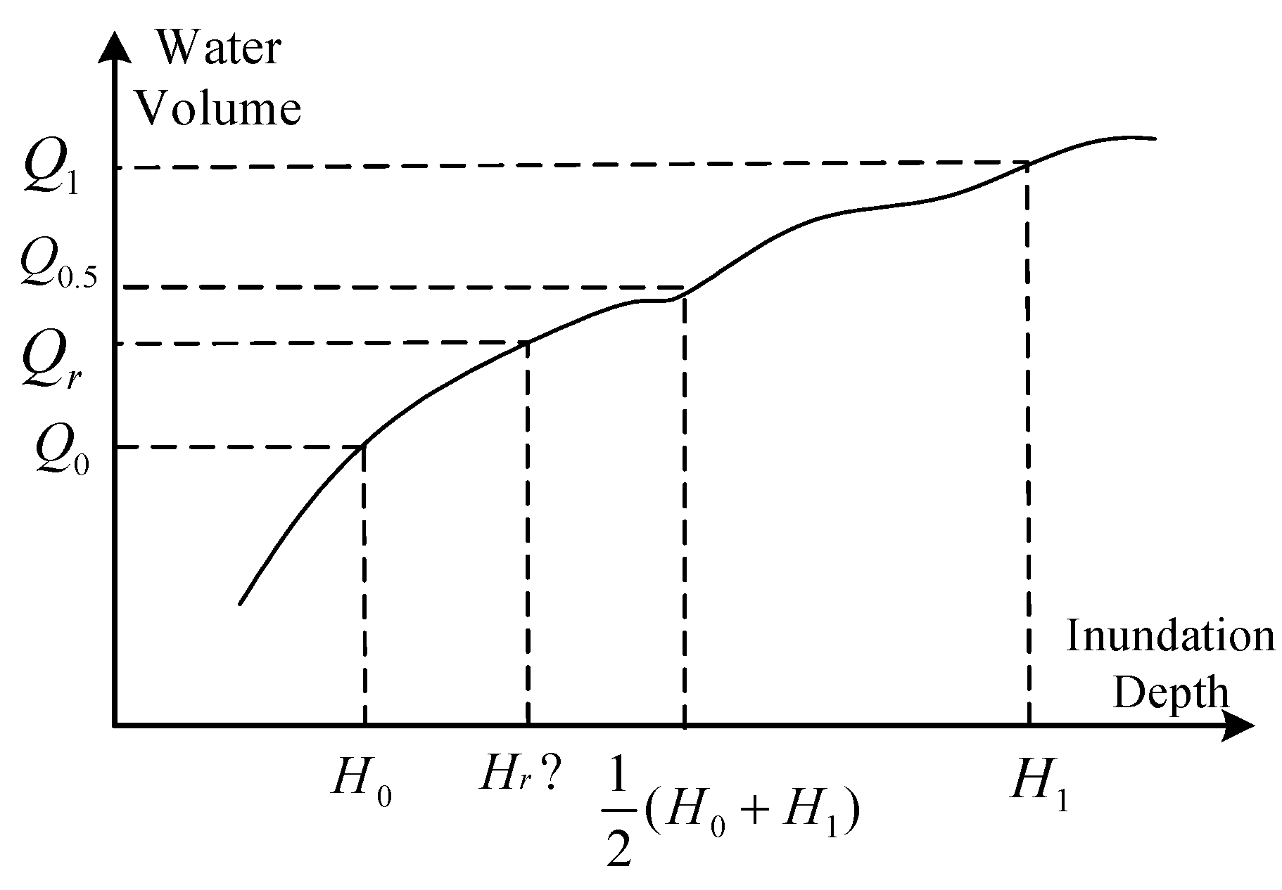
3.4. Inundation Depth Calculation

The accumulated excess water volume on the terrain converts to the runoff water volume to inundate urban surface. This is equal to the water volume between water surface and urban surface at a certain time. This can be expressed as Equations (8) and (9).
Qr = ʃA (Hw - Hg)ds
Qa = Qr
where, Qr is the runoff water volume on the urban surface (m3); A is the inundation area (m2); ds is the basic integral area (m2); Hw is the inundated water surface elevation (m); and Hg is the ground elevation (m).
Referring to Equations (6)–(9), the inundation water level can be expressed associating with rainfall, terrain features and drainage parameters. Analytical solution cannot be evidently obtained to solve the equations due to the complexity of the urban surfaces. Numerical solutions through dichotomy [51] are employed. Each triangle serves as the calculation unit (triangular prism shown as in Figure 9) for obtaining the water level. The detailed algorithm includes the following procedures (illustration shown in Figure 10).
(1)
Initialize the maximum (H1) and minimum (H0) inundation depth;
(2)
Within each basin which consist of triangular-prism sets, calculate the water volume Q0, Q1 under the inundation depth of H0 and H1;
(3)
If Q0 = Qr then Hr = H0; else if Q1 = Qr then Hr = H1; otherwise calculate the water volume Q0.5 under the water surface of H0.5, which equals Water 06 01151 i006;
(4)
If Q0.5 = Qr, then Hr = H0.5; else if Q0.5 > Qr, then Q1 = Q0.5 and H1 = H0.5; otherwise if Q0.5 < Qr, then Q0 = Q0.5 and H0 = H0.5;
(5)
Go to Step (2) until obtaining the Hr.
Therefore, continuous inundation can be divided into discrete time intervals to simulate inundation scenarios during the storm event. Each scenario can obtain the water surface (including inundation extent and water depth) by employing the above methods.
Figure 9. Triangular-prism sets of the depression and three inundation phases of one triangular-prism blue represents the accumulated water, h1, h2, h3 representing the water submerged in one, two, and three nodes of the bottom triangle, respectively. (a) Triangular-prism sets of the depression; (b) submerged one node; (c) submerged two nodes; (d) submerged three nodes.
Water 06 01151 g009
Figure 10. Dichotomy numerical solving iteration method to obtain inundation depth Hr.
Water 06 01151 g010

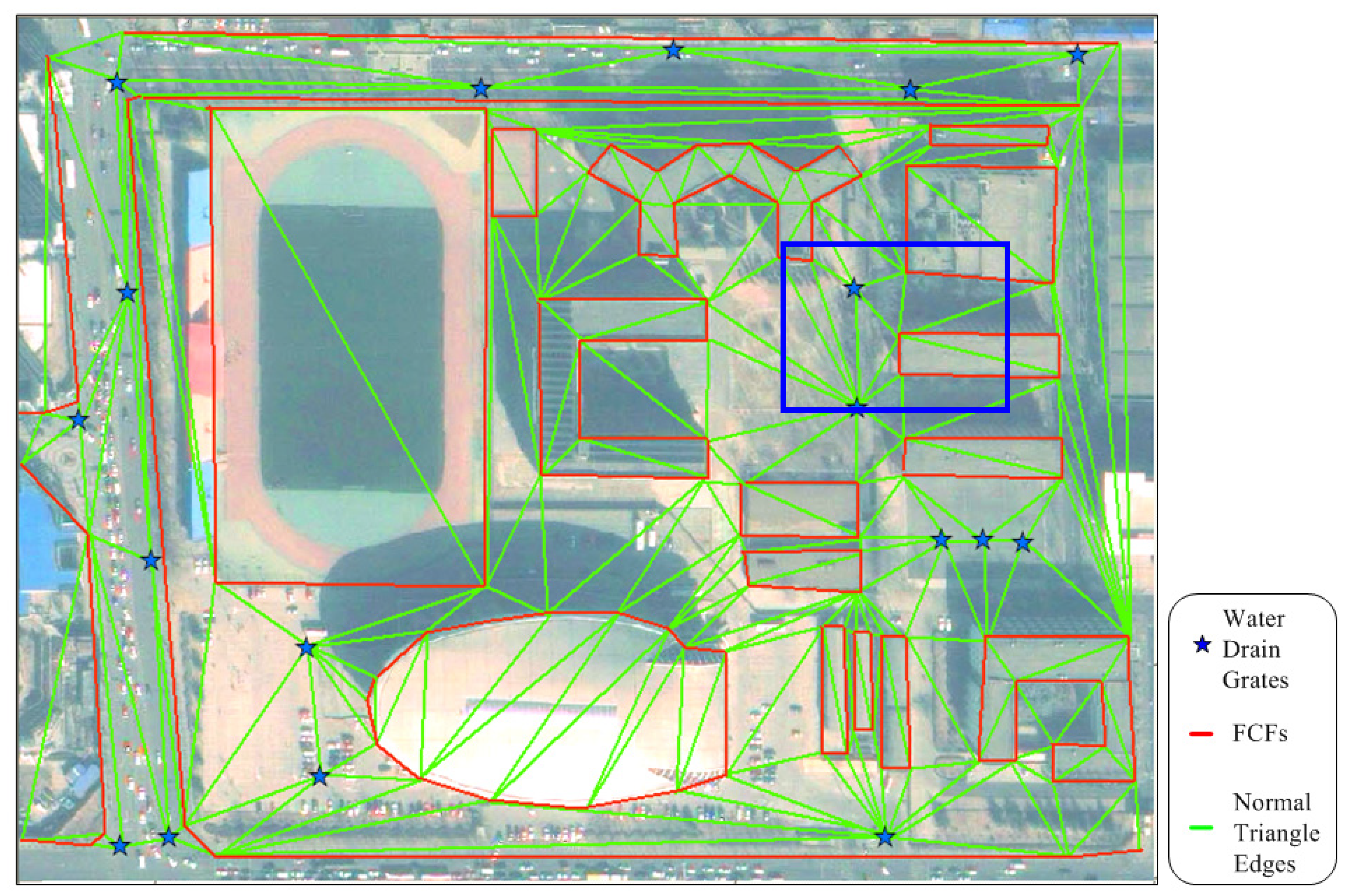
4. BNU Main Campus Case Study

4.1. Urban Surface Modeling

Located between the second and third rings of municipal Beijing, China, campus of BNU is a typical urban surface. The campus experiences severe inundation storm events on an annual basis, particularly on the FuRen Road in front of the Geography & Remote Sensing Building. The drainage system around FuRen road existing faults have been shown through an investigation with the staff at the logistics management center of BNU.
This urban surface was surveyed by total station, an S3 digital level according to level-IV national surveying standard and the 1:500 national data capturing standard. The total length closing error of traverse surveying result was 0.1528 m. The relative length closing error of traverse is 1/1,7127 less than the surveying standard error (1/10000). The closed error of elevation was 8 mm. These are all within the range of national 1:500 cartography standard. The surveyed data were organized with Shapefile (with elevation z value) format shown as in Figure 11.
Figure 11. Surveyed data of the main campus of BNU with Shapefile organization.
Water 06 01151 g011
Utilizing the modeling method in Section 2.2, the BNU main campus terrain is represented as shown in Figure 12. The FCFs can be modeled in detail by the CD-TIN and the buildings and other man-made structures can be seamlessly coupled in the CD-TIN terrain [52]; also, the full topology relationship of CD-TIN facilitates further analysis of inundation. As Figure 13 shows, for better understanding the representation of CD-TIN, we add the aerial imagery of the BNU main campus. From the imagery, we can see the FCFs are well represented in the model. Furthermore, the zoomed regions demonstrate the effective modeling of buildings, street curbs and central garden by employing the CD-TIN model.
Figure 12. BNU main campus surface representations with CD-TIN at different draw modes and views.
Water 06 01151 g012
Figure 13. BNU main campus CD-TIN representations with aerial imagery.
Water 06 01151 g013

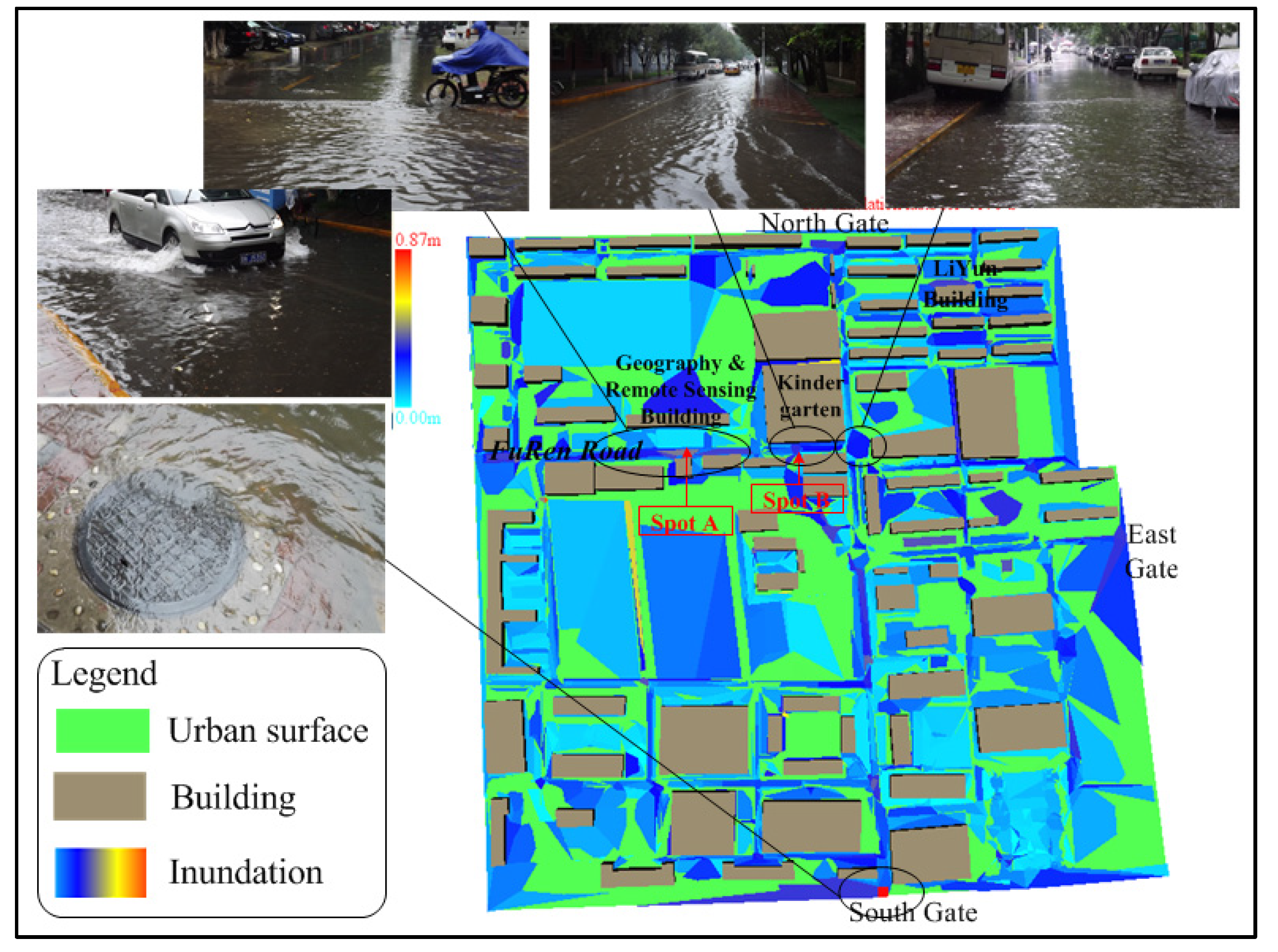
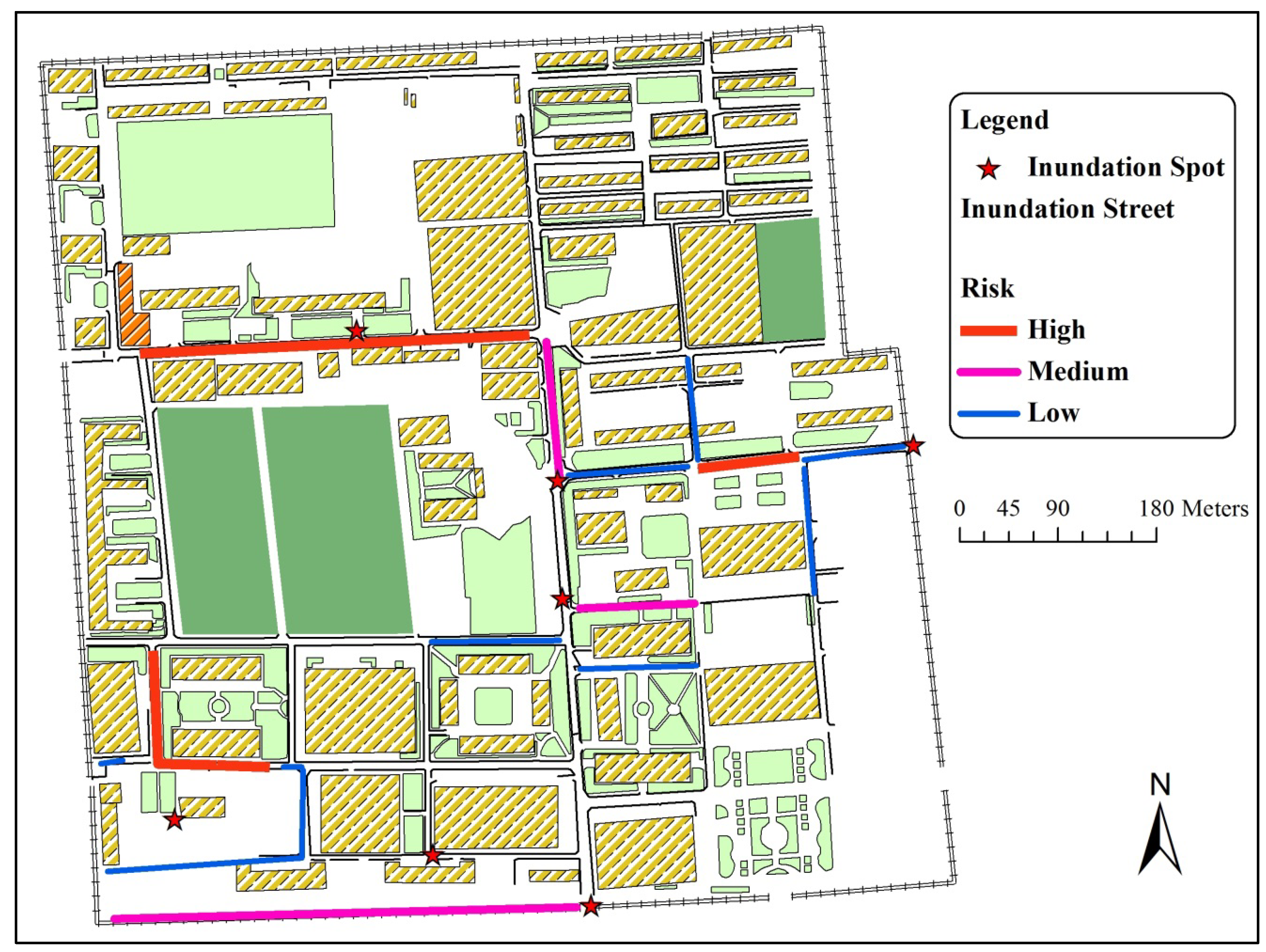
4.2. Inundation Simulation
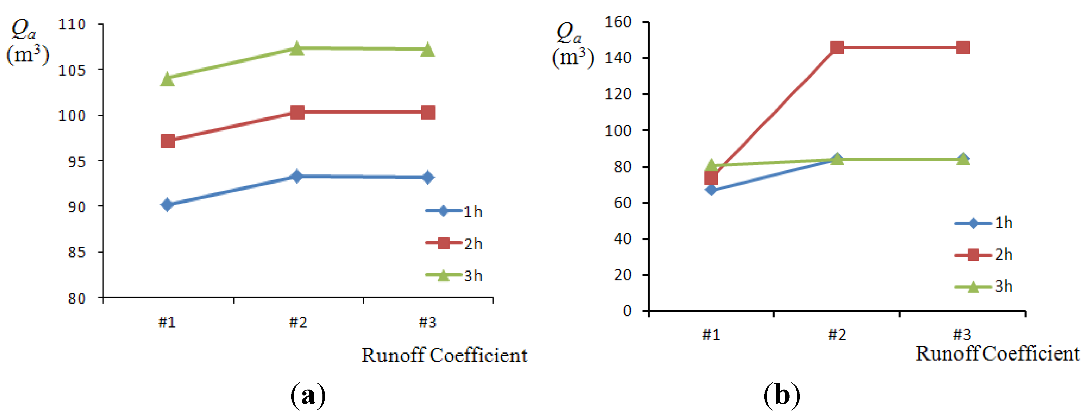
The storm event on 21 July 2011 in Beijing (called the “7.21” storm) was a 61-year-frequency high storm rainfall event, and it has affected approximately 1.9 million people and caused 1.6 billion dollars in economic loss [53]. The “7.21” storm event reappeared as the application case on the main campus of BNU. According to a related report [54], the average precipitation of “7.21” storm is as high as 215 mm in 12 h, with a 61-year frequency. The observed duration of the storm was approximately 3 h in the domain of BNU. According to Equation (2), calculated precipitation of this storm event is 0.76 mm/min. The runoff coefficients of different land types adopt their corresponding historical values, shown in Table 2 [55]. During the storm event, drain pipes may be filled prior to the storm or reach capacity quickly after the storm begins. When inundation occurs, this research assumes drain pipes at their full capacity. Referring to record materials from the BNU logistics management center, the full capacity of drain pipes can be calculated by Equation (5).
To simulate the “7.21” storm, the inundation scenario can be timely acquired by employing the runoff coefficient as #2 (Experiment environment: Intel®Core™2 Duo CPU p8600 @ 2.4GHz, 1.93GB RAM). As shown in Figure 14, severely inundated spots are labeled: FuRen Road in front of the Geography Building (labeled as A), Kindergarten (labeled as B), LiYun Building, East gate, North gate, and South gate. To validate the simulation result, we compare the inundation scenario with in-situ captured photos by the authors and BNU logistics office during the storm event. From comparisons in Figure 14, the simulated inundation is generally consistent with the real scenario. Meanwhile, the maximum inundation depth of two severely submerged spots A and B have been captured during the event. The comparison is given as shown in Table 3, which employs the runoff coefficient value #1, #2, #3 in Table 2 for simulation, respectively.
Figure 14. BNU main campus “7.21 storm” inundation scenario and comparison with in-situ captured photos. The most severe submerged spots are labelled with A and B on the FuRen Road in front of Geography Building and Kindergarten.
Water 06 01151 g014
The lack of abundant in-situ observed data of the “7.21” event at the test site means that the ensuing modeling exercise takes the form of a sensitivity analysis. To analyze the sensitivity of runoff coefficient, three group runoff coefficients (#1, #2, #3, as shown in Table 2) are employed to simulate the difference. The water depression where A is located (called depression An), whose contribution area is about 5374 m2, is a composite of grass land and road surface. While the water depression where B is located (called depression Bn), whose contribution area is about 409 m2, is a composite of road surface and building surface. We conduct the simulation to obtain the accumulated water volume with different runoff coefficients (#1, #2, #3) and rainfall duration (1 h, 2 h, 3 h). As shown in Figure 15: (1) the same underlying land type can yield more accumulated water varying with larger coefficients, vice versa; (2) An has the similar accumulative pattern that the accumulative volume rises with the increasing rainfall duration on the same underlying surface with the same coefficient; whereas, the accumulative pattern of Bn is irregular due to uncertainty of in-flow of water from adjacent depressions. As Table 3 shows, the simulated inundation depths are compared with the in-situ captured maximum inundation depth. From that we know several facts: (1) The variety of runoff coefficient has certain influence on the simulation that depends on urban surface; (2) Due to An composite of grass land and road surface, the yield water of unit area on the grass land is less than that on the road surface. Thus, the simulated accumulative water volume is relatively small so that the water depth is relatively small; (3) Bn is a composite of road surface and building surface with a similar runoff coefficient, and so the simulation result should be stable. However, the simulated depth with coefficient value #2 dramatically changes in that the accumulative water is affected by the water flow from adjacent water depressions.
Figure 15. Excess runoff volume with different runoff coefficient at rainfall duration of 1 h, 2 h, and 3 h, respectively. (a) The accumulated water in An; (b) the accumulated water in Bn.
Water 06 01151 g015
Table 3. Inundation water depth and simulation result (Unit: cm).
Used Runoff CoefficientRecord Depth ASimulation ResultRelative ErrorRecord Depth BSimulation ResultRelative Error
Value #1423516.7%36345.6%
Value #242379.6%36338.3%
Value #342389.5%36338.3%
From Table 3, the conclusion can be made that different runoff coefficients (as value #1, #2, #3) can influence the simulated water depth but not dramatically. From relative errors, we know the simulated results generally agree with the record data. Although other in-situ water depths of inundated spots are not captured, the result can be validated according to the inundation spot report by the BNU logistics division office. If more in-situ data were captured, the quantitative analysis conclusion provided could be more reliable and persuasive.
For further validation of the simulation result, we compare the result with the inundation risk perception map. As shown in Figure 16, the map is generated from the questionnaires of students and local residents by the Disaster Risk Management Center of BNU. Furthermore, the questionnaires mainly focus on the “7.21” storm event. We need to explain that the inundation risk map is based on the captured data; hence, the areas on Figure 16 without risk labels do not mean any inundation, just lack of captured data. However, this map can validate our model simulation result to a certain extent. To compare Figure 14 with Figure 16, we know that: (1) the high inundation spots basically agree with the simulated results, especially at the spot A, B, and south gate of BNU; (2) the high risk of inundation streets are FuRen Road and the street south of the south gate, and both coincide with the simulation result.
Figure 16. Inundation risk map from questionnaires for the “7.21” storm event.
Water 06 01151 g016

5. Conclusions and Discussion

Referring to FCFs, we employed the CD-TIN to model urban surface in detail. An edge flow mode was utilized to subdivide the potential urban water depressions into computational depression polygons. Storm-runoff yield was evaluated through mass conservation principles to calculate the volume of rainfall, runoff and drainage. Water confluence between neighboring depressions was provided when the water level exceeded the outlets. Numerical solution through a dichotomy was employed to obtain the inundation water levels. During storm events, continuous inundation processes can be divided into different time intervals to obtain the inundation extent and submerged water depth. Simulation experiments of the BNU main campus “7.21” storm event in 2011 were conducted to validate the usability and suitability of the proposed methods. The results show that CD-TIN based methods are reasonable, effective, and less time-consuming, thus providing a practical new method for urban inundation simulation. Hence, the characteristics of the proposed model can be summarized as follows:
(a)
The model focuses on the detailed surveyed urban surfaces with fine CD-TIN representation instead of raster. It couples the fine constrained urban features, such as street curbs, road cambers, ans water drain grates, which greatly influence urban water flow;
(b)
The model can handle the storm flood with a lack of detailed drainage data, especially the discharge of the subsurface drainage system, or urban environments with a built-in sewer system;
(c)
The model employs the GIS-based dichotomy numerical simulation method, which avoids the time-consuming problem of 1D or 2D equation numerical calculation. It can provide a practical rapid inundation solution for urban storm flood simulation.
Due to the complexity of urban surface and modeling elements, some simplifications must be noted. This research accepted the flat-water concept which does not consider physical hydrodynamics. Therefore, several assumptions and simplifications must be discussed. (1) Physical factors such as gravity and friction were not considered; mass conservation was applied as the governing equation; (2) Although the historical value of surface friction and runoff were adopted from previous researches, this may have overestimated the total volume of distributed surface runoff and inundation conditions; (3) Any interactions between the surface flow and the underground sewer system were not considered. All conveyance were assumed to be equal to design conveyances (a permanent flow rate), even though they actually vary with time during and after a storm event. The conveyance could be very low at the beginning and gradually reach the full permanent flow. Thus, the assumption of permanent sewer conveyable full flow leads to underestimation of flood water volume, so does inundation depth [22]; (4) The unit rainfall of this method input is typically appropriate for a small study area [22] such as BNU main campus, instead of spatial variation rainfall for a large study area; (5) The input parameters of the proposed methods such as rainfall, runoff capacity and drainage system capacity were all based on historical or empirical values from previous researches and engineering standards. These parameters can influence the accumulated excess water volume on the surface, as well as the final inundation result.
Although this research has a number of assumptions and limitations, it is useful for urban storm inundation risk analysis, urban drainage design and emergency preparation because of its more timely performance, fine representation of urban surface and minimal drainage data requirements during a storm. This method can incorporate real world sewer system situations including the dynamics of drainage systems and the interaction between surface and subsurface, and flow without changing the concept and framework of the proposed methods in our future work.

Acknowledgments

We would like to acknowledge the financial support from the Beijing Municipal Natural Science Foundation Key Program (No. 8111003), the National Basic Research Program of China (No. 2011CB707102) and the Fundamental Research Funds for Central Universities (No. 105565GK). We would like to acknowledge the BNU logistics division office for the drainage data and inundation photos of the BNU in the “7.21” storm event, and the Disaster Risk Management Center of BNU for their questionnaires and inundation risk map.

Author Contributions

Zhifeng Li designed the inundation model and wrote the original manuscript of the paper. Lixin Wu proposed the conceptual framework of the paper and revised the manuscript. Wei Zhu provided the drainage data and conducted the experiment of Beijing Normal University (BNU) “7.21” storm event. Miaole Hou surveyed the detailed urban surface and organized them into database. Yizhou Yang wrote the C++ code for the simulation algorithms. Jianchun Zheng provided the inundation validation analysis for simulation of BNU “7.21” inundation.

Conflicts of Interest

The authors declare no conflict of interest.

References

  1. Fewtrell, T.J.; Duncan, A.; Sampson, C.C.; Neal, J.C.; Bates, P.D. Benchmarking urban flood models of varying complexity and scale using high resolution terrestrial LiDAR data. Phys. Chem. Earth Parts A B C 2011, 36, 281–291. [Google Scholar] [CrossRef]
  2. Smith, M.B. Comment on ‘Analysis and modeling of flooding in urban drainage systems’. J. Hydrol. 2006, 317, 355–363. [Google Scholar] [CrossRef]
  3. Schmitt, T.G.; Thomas, M.; Ettrich, N. Analysis and modeling of flooding in urban drainage systems. J. Hydrol. 2004, 299, 300–311. [Google Scholar] [CrossRef]
  4. Maksimović, Č.; Prodanović, D.; Boonya-Aroonnet, R.S.; Leitão, J.P.; Djordjević, S.; Allitt, D.R. Overland flow and pathway analysis for modelling of urban pluvial flooding. J. hydraul. Res. 2009, 47, 512–523. [Google Scholar] [CrossRef]
  5. Djordjević, S.; Prodanović, D.; Maksimović, C.; Ivetić, M.; Savić, D. SIPSON—Simulation of interaction between pipe flow and surface overland flow in networks. Water Sci. Technol. 2005, 52, 275–289. [Google Scholar]
  6. Djordjević, S.; Prodanović, D.; Maksimović, Č. An approach to simulation of dual drainage. Water Sci. Technol. 1999, 39, 95–103. [Google Scholar] [CrossRef]
  7. Carr, R.S.; Smith, G.P. Linking of 2D and Pipe Hydraulic Models at Fine Spatial Scales. In Proceedings of the 4th International Conference on Water Sensitive Urban Design, Melbourne, Australia, 3–7 April 2006; pp. 888–895.
  8. Chen, A.; Hsu, M.; Chen, T.; Chang, T.J. An integrated inundation model for highly developed urban areas. Water Sci. Technol. 2005, 51, 221–230. [Google Scholar]
  9. Chen, A.S.; Djordjevic, S.; Leandro, J.; Savic, D. The Urban Inundation Model with Bidirectional Flow Interaction between 2D Overland Surface and 1D Sewer Networks. In Proceedings of the 6th International Conference on Sustainable Techniques and Strategies in Urban Water Management (NOVATECH), Lyon, France, 25–28 June 2007; pp. 465–472.
  10. Dey, A.K.; Kamioka, S. An integrated modeling approach to predict flooding on urban basin. Water Sci. Technol. 2007, 55, 19–29. [Google Scholar]
  11. Seyoum, S.; Vojinovic, Z.; Price, R.; Weesakul, S. Coupled 1D and noninertia 2D flood inundation model for simulation of urban flooding. J. Hydraul. Eng. 2012, 138, 23–34. [Google Scholar] [CrossRef]
  12. Li, W.; Chen, Q.; Mao, J. Development of 1D and 2D coupled model to simulate urban inundation: An application to Beijing Olympic Village. Chin. Sci. Bull. 2009, 54, 1613–1621. [Google Scholar] [CrossRef]
  13. Bates, P.D.; De Roo, A.P.J. A simple raster-based model for flood inundation simulation. J. Hydrol. 2000, 236, 54–77. [Google Scholar] [CrossRef]
  14. Hunter, N.M.; Horritt, M.S.; Bates, P.D.; Wilson, M.D.; Werner, M.G.F. An adaptive time step solution for raster-based storage cell modelling of floodplain inundation. Adv. Water Resour. 2005, 28, 975–991. [Google Scholar] [CrossRef]
  15. Leandro, J.; Chen, A.; Djordjević, S.; Savić, D.D.A. Comparison of 1D/1D and 1D/2D coupled (Sewer/Surface) hydraulic models for urban flood simulation. J. Hydraul. Eng. 2009, 135, 495–504. [Google Scholar] [CrossRef]
  16. Leandro, J.; Djordjević, S.; Chen, A.S.; Savić, D.A.; Stanić, M. Calibration of a 1D/1D urban flood model using 1D/2D model results in the absence of field data. Water Sci. Technol. 2011, 64, 1016–1024. [Google Scholar] [CrossRef]
  17. Chen, A.S.; Evans, B.; Djordjević, S.; Savić, D.A. Multi-layered coarse grid modelling in 2D urban flood simulations. J. Hydrol. 2012, 470–471, 1–11. [Google Scholar] [CrossRef] [Green Version]
  18. Hunter, N.; Bates, P.; Neelz, S.; Pender, G.; Villanueva, I.; Wright, N.; Liang, D.; Falconer, R.; Lin, B.; Waller, S. Benchmarking 2D hydraulic models for urban flooding. Proc. ICE Water Manag. 2008, 161, 13–30. [Google Scholar] [CrossRef] [Green Version]
  19. Neal, J.; Fewtrell, T.; Trigg, M. Parallelisation of storage cell flood models using OpenMP. Environ. Model. Softw. 2009, 24, 872–877. [Google Scholar] [CrossRef]
  20. Kalyanapu, A.J.; Shankar, S.; Pardyjak, E.R.; Judi, D.R.; Burian, S.J. Assessment of GPU computational enhancement to a 2D flood model. Environ. Model. Softw. 2011, 26, 1009–1016. [Google Scholar] [CrossRef]
  21. Néelz, S.; Pender, G. Benchmarking of 2D Hydraulic Modeling Packages; Environment Agency: Bristol, UK, 2010. [Google Scholar]
  22. Chen, J.; Hill, A.; Urbano, L.D. A GIS-based model for urban flood inundation. J. Hydrol. 2009, 373, 184–192. [Google Scholar] [CrossRef]
  23. Zerger, A.; Smith, D.I.; Hunter, G.J.; Jones, S.D. Riding the storm: A comparison of uncertainty modelling techniques for storm surge risk management. Appl. Geogr. 2002, 22, 307–330. [Google Scholar] [CrossRef]
  24. Zerger, A. Examining GIS decision utility for natural hazard risk modelling. Environ. Model. Softw. 2002, 17, 287–294. [Google Scholar] [CrossRef]
  25. Bates, P.D.; Horritt, M.S.; Fewtrell, T.J. A simple inertial formulation of the shallow water equations for efficient two-dimensional flood inundation modelling. J. Hydrol. 2000, 387, 33–35. [Google Scholar]
  26. Liu, Y.; Snoeyink, J. Flooding Triangulated Terrain. In Developments in Spatial Data Handling; Springer Berlin: Heidelberg, Germany, 2005; pp. 137–148. [Google Scholar]
  27. Zhou, Q.; Liu, X. Error assessment of grid-based flow routing algorithms used in hydrological models. Int. J. Geogr. Inf. Sci. 2002, 16, 819–842. [Google Scholar] [CrossRef]
  28. Liu, X.J.; Wang, Y.J.; Ren, Z. Algorithm for extracting drainage network based on triangulated irregular network. J. Hydraul. Eng. 2008, 39, 27–35. (In Chinese) [Google Scholar]
  29. Leitão, J.P.; Boonya-aroonnet, S.; Prodanovic, D.; Maksimovic, C. The influence of digital elevation model resolution on overland flow networks for modelling urban pluvial flooding. Water Sci. Technol. 2009, 60, 3137–3149. [Google Scholar] [CrossRef]
  30. Chou, T.-Y.; Lin, W.-T.; Lin, C.-Y.; Chou, W.-C.; Huang, P.-H. Application of the PROMETHEE technique to determine depression outlet location and flow direction in DEM. J. Hydrol. 2004, 287, 49–61. [Google Scholar] [CrossRef]
  31. Martz, L.W.; Garbrecht, J. The treatment of flat areas and depressions in automated drainage analysis of raster digital elevation models. Hydrol. Processes 1998, 12, 843–855. [Google Scholar] [CrossRef]
  32. Marks, D.; Dozier, J.; Frew, J. Automated basin delineation from digital elevation data. Geo Process. 1984, 2, 299–311. [Google Scholar]
  33. Vogt, J.V.; Colombo, R.; Bertolo, F. Deriving drainage networks and catchment boundaries: A new methodology combining digital elevation data and environmental characteristics. Geomorphology 2003, 53, 281–298. [Google Scholar] [CrossRef]
  34. Lin, W.T.; Chou, W.C.; Lin, C.Y.; Huang, P.H.; Tsai, J. WinBasin: Using improved algorithms and the GIS technique for automated watershed modelling analysis from digital elevation models. Int. J. Geogr. Inf. Sci. 2008, 22, 47–69. [Google Scholar] [CrossRef]
  35. Theobald, D.M.; Goodchild, M.F. Artifacts of TIN-based surface flow modeling. Proc. GIS LIS 90 1990, 2, 955–967. [Google Scholar]
  36. Bänninger, D. Technical note: Water flow routing on irregular meshes. Hydrol. Earth Syst. Sci. Discuss. 2006, 3, 3675–3689. [Google Scholar] [CrossRef]
  37. Tucker, G.E.; Lancaster, S.T.; Gasparini, N.M.; Bras, R.L.; Rybarczyk, S.M. An object-oriented framework for distributed hydrologic and geomorphic modeling using triangulated irregular networks. Comput. Geosci. 2001, 27, 959–973. [Google Scholar] [CrossRef]
  38. Ivanov, V.Y.; Vivoni, E.R.; Bras, R.L.; Entekhabi, D. Catchment hydrologic response with a fully distributed triangulated irregular network model. Water Resour. Res. 2004, 40. [Google Scholar] [CrossRef]
  39. Sampson, C.C.; Fewtrell, T.J.; Duncan, A.; Shaad, K.; Horritt, M.S.; Bates, P.D. Use of terrestrial laser scanning data to drive decimetric resolution urban inundation models. Adv. Water Resour. 2012, 41, 1–17. [Google Scholar] [CrossRef]
  40. Mason, D.C.; Horritt, M.S.; Hunter, N.M.; Bates, P.D. Use of fused airborne scanning laser altimetry and digital map data for urban flood modelling. Hydrol. Processes 2007, 21, 1436–1447. [Google Scholar] [CrossRef]
  41. Fewtrell, T.J.; Bates, P.D.; Horritt, M.; Hunter, N.M. Evaluating the effect of scale in flood inundation modelling in urban environments. Hydrol. Processes 2008, 22, 5107–5118. [Google Scholar] [CrossRef]
  42. Wu, L.; Shi, W. Principle and Algorithem of GIS; Science Press: Beijing, China, 2003; pp. 156–160. [Google Scholar]
  43. Frank, A.U.; Palmer, B.; Robinson, V. Formal Methods for the Accurate Definition of Some Fundamental Terms in Physical Geography. In Proceedings of 2nd International Symposium on Spatial Data Handling, Seattle, WA, USA, 5–10 July 1986; pp. 583–599.
  44. Apirumanekul, C. Modeling of Urban Flooding in Dhaka City; No. WM-00-13; Asian Institute of Technology: Bangkok, Thailand, 2001. [Google Scholar]
  45. Beijing General Municipal Engineering Design and Research Institute. Water Supply and Drainage Design Manual: Volume 5th Urban Drainage; China Building Industry Press: Beijing, China, 2004. [Google Scholar]
  46. Holtan, H.N. Time condensation in hydrograph analysis. Trans. Am. Geophys. Union 1945, 26, 407–413. [Google Scholar] [CrossRef]
  47. Sharp, A.L.; Holtan, H.N. Extension of graphic methods of analysis of sprinkled-plot hydrographs to the analysis of hydrographs of control plots and small homogeneous watersheds. Trans. Am. Geophys. Union 1942, 23, 578–593. [Google Scholar] [CrossRef]
  48. Mays, L.W. Water Resources Engineering; Wiley: New York, NY, USA, 2001. [Google Scholar]
  49. Hsu, M.H.; Chen, S.H.; Chang, T.J. Inundation simulation for urban drainage basin with storm sewer system. J. Hydrol. 2000, 234, 21–37. [Google Scholar] [CrossRef] [Green Version]
  50. Hao, Z.; Li, L.; Wang, J.; Luo, J. Distributed Hydrological Model Theory and Method; Science Press: Beijing, China, 2010; pp. 256–260. [Google Scholar]
  51. Li, Z.F.; Wu, L.X.; Zhang, Z.X.; Xu, Z.H. Triangular-Prism-Based Algorithm on Urban Flood Inundation Simulation by Employing Dichotomy Numerical Solution. In Proceedings of International Geoscience and Remote Sensing Symposium (IGARSS), Melbourne, Austrilia, 21–26 July 2013; 2013; pp. 790–793. [Google Scholar]
  52. Wu, L.X.; Wang, Y.B.; Shi, W.Z. Integral ear elimination and virtual point-based updating algorithms for constrained Delaunay TIN. Sci. China Ser. E Technol. Sci. 2008, 51, 135–144. [Google Scholar] [CrossRef]
  53. Beijing “7.21” Storm Event. Available online: http://www.weather.com.cn/zt/kpzt/696656.shtml (accessed on 20 August 2013). (In Chinese)
  54. Beijing encountered the strongest storm with 61 year return period and the average precipitation as high as 215 mm. Available online: http://news.sohu.com/20120722/n348744539.shtml (accessed on 20 August 2013). (In Chinese)
  55. Ministry of Development of the People’s Republic of China. Outdoor Drainage Design Standard (GB 50014–2006); China Planning Press: Beijing, China, 2011.

