Article

An Analysis of Land Use Change Dynamics and Its Impacts on Hydrological Processes in the Jialing River Basin

1
College of Hydrology and Water Resources, Hohai University, No. 1 Xikang Road, Nanjing 210098, Jiangsu Province, China
2
National Engineering Research Center of Water Resources Efficient Utilization and Engineering Safety, Hohai University, No. 1 Xikang Road, Nanjing 210098, Jiangsu Province, China
3
Changjiang Water Resources Protection Institute, No. 515 Qintai Street, Wuhan 430051, Hubei Province, China
*
Author to whom correspondence should be addressed.
Water 2014, 6(12), 3758-3782; https://doi.org/10.3390/w6123758
Submission received: 1 July 2014 / Revised: 10 November 2014 / Accepted: 25 November 2014 / Published: 4 December 2014

Abstract

:
Land use changes are important aspects of global change and affect regional water cycles, environmental quality, biodiversity and terrestrial ecosystems. To understand the temporal and spatial land use change in the Jialing River Basin and its impacts on the hydrological cycle, land use change models and the variable infiltration capacity (VIC) model were applied separately to the Jialing River Basin. Real change and final change were analyzed to determine the consequences of land use changes and their hydrological consequences. Real change is defined as the total variation during a fixed period, including increases and decreases. Thus, real change is the sum of the absolute values of the decrease and the increase. Final change is defined as the difference between the beginning and end of a given period for a specific factor. Overall, the amounts of settlement and shrub land area changed significantly in the entire Jialing River (with final change rates of 20.77% and −16.07%, respectively, and real change rates of 34.2% and 30.1%, respectively, from 1985 to 1995, as well as final and real change rates of 29.37%, 12.40%, 39.9% and 32.8%, respectively, from 1995 to 2000). Compared with the final change, the real change highlighted the rate of change and the change in woodland area. The land use changes in the Lueyang (LY), Shehong (SH) and Fengtan (FT) subcatchments were more dynamic than in the other subcatchments. The economy, population and macro-policy were the main factors responsible for driving the land use changes. The decrease in woodland area in the LY subcatchment corresponded with an increase in evapotranspiration (ET) and with decreases in the other hydrological elements. Overall, the final changes in the hydrological elements in the LY, SH and FT subcatchments were not significant due to the average and compensation effects. The LY subcatchment was mainly affected by the average effect, whereas the SH and FT subcatchments were affected by the average and compensation effects. The use of real change can increase the detectability of hydrological elements changes caused by land use change in SH and FT. The results of this study provide new insights regarding the examination of the effects of land use changes on hydrological regimes. These results are useful for land use planners and water resource managers.

Graphical Abstract

1. Introduction

With the intensification of several global issues, including increasing population, food shortages, environmental pollution and climate change, global change has become one of the most popular areas of research, within which land use change is particularly important [1]. To survive and develop, humans have explored new forms of land use, resulting in land use changes.
Many studies have shown that land use changes are closely linked to hydrological processes. The main effects of land use changes on the water cycle are changes in evapotranspiration (ET), changes in the soil’s ability to hold water and changes in the abilities of vegetation to intercept precipitation [2]. In addition, land use change extensively modifies the pathway and the surface roughness and then affects the timing of runoff, which leads to changes in the river flow (for example, flood peak appearance time and volume).
Dunn and Mackay [3], Matheussen et al. [4], Olchev et al. [5], Jin [6] and Mao and Cherkauer [7] have detected changes in ET due to land use changes and have shown that decreases in cover or damage to woodlands result in clear decreases in ET. Andraski [8], Shi and Li [9] and Krause [10] studied soil water variation in the field. Normally, after vegetation is removed, the distribution of roots becomes shallower, the soil porosity (especially the non-capillary porosity) decreases and the soil moisture-holding capacity decreases. Legesse et al. [11], Coe et al. [12], Savary et al. [13] and Schilling et al. [14] have performed related studies regarding the changes in runoff under different land use conditions and have obtained similar results. These authors observed that ET is stronger from woodlands than from other types of land. In addition, forested catchments have greater infiltration rates, which may decrease catchment runoff. Many other researchers have studied the effects of land use changes on river flow [15,16,17,18,19], and most of them have indicated that intensified afforestation will reduce both runoff peak and total runoff volume.
The methods used in these studies primarily included comparative analyses and hydrological modeling. With the development of physically-based and distributed/semi-distributed hydrology models, such as the Systeme Hydrologique Europeen (SHE), Soil and Water Assessment Tool (SWAT) and variable infiltration capacity (VIC) models, more researchers [20,21,22,23] are increasingly utilizing hydrological models to interpret and predict hydrological responses to land use changes. Although these studies provide a feasible method for drawing conclusions or addressing hydrological and water resource problems that result from land use change, they do not focus on land use dynamics.
The Jialing River is an important upstream watershed on the Yangtze River drainage basin, and its surrounding area is undergoing dramatic population growth with rapid economic development. In addition, various land use policies are being developed in this region, including the “Yangtze River Management” project and the return of croplands to forest and grasslands (RCFG), which were implemented in the 1980s and at the end of the 1990s, respectively. The land use dynamics along the Jialing River have changed significantly. Although many researchers [24,25,26,27,28,29] have examined the dynamics of land use change in this area, few studies have assessed the effects of these changes from a hydrological perspective. Thus, it is important to analyze land use changes and their impacts on the hydrological processes in this area.
This study uses land use change models to analyze and evaluate temporal and spatial land use changes. In addition, the VIC model was applied in this study to simulate hydrological elements under different land use types. Finally, this study assesses the impacts of land use changes on the hydrological regimes.
The main objectives of this study are as follows:
(1)
To clarify how land use has changed in the Jialing River Basin and to identify hot spots of land use change;
(2)
To present a new viewpoint for examining hydrological regime changes due to land use changes.

2. Materials and Methods

2.1. Study Area and Data

2.1.1. Study Area

The Jialing River is the largest branch of the Yangtze River and is approximately 1120 km long. The Jialing Basin covers an area of approximately 160,000 km2 within a geographical range of 29°17'30" N–34°28'11" N and 102°35'36" E–109°01'08" E (Figure 1). This region is located in the subtropical zone and has a humid monsoon climate. It has an annual average daily maximum temperature of 19.4 °C, an annual average daily minimum temperature of 4.3 °C, an average wind speed of 1.1 m/s and an average annual precipitation of 931 mm.

2.1.2. Materials

Three periods (1985, 1995, 2000) of land use were obtained from the Data Center for Resources and Environmental Sciences, Chinese Academy of Sciences (RESDC) [30]. This dataset was created by the Chinese Academy of Sciences (CAS) at 1-km resolution with the National Land Resource Classification System of China based on land use maps for the 1980s, 1995 and 2000 provided by the National 1:100,000 Land Use Database. The land use type interpretation resolution of the National 1:100,000 Land Use Database is as high as 92.92% according to assessments based on field surveys. These data were first used to analyze the dynamics of land use changes in the study area and were then used to obtain land use change scenarios, using the VIC model to assess the effects of land use changes on subwatershed hydrological regimes. Because the CAS classification system differs from the University of Maryland land cover classification (UMD), which is compatible with the VIC model, the conversion method used by Zhang et al. [31] was adopted. Land use types were reclassified into cropland, woodland, shrubland, grassland, water, settlement and bare ground.
Figure 1. Location of the Jialing River Basin.
Water 06 03758 g001
Notes: LMS: Langmusi; PW: Pingwu; GY: Guangyuan; MY: Mianyang; LZ: Langzhong; BZ: Bazhong; WY: Wanyuan; SN: Suining; NC: Nanchong; DX: Daxian; SPB: Shapingba; WD: Wudu; LY: Lveyang; SLB: Sanleiba; JYT: Jinyintai; SH: Shehong; FT: Fengtan; GDK: Goudukou; BB: Beibei.
The following data are required for the VIC model:
The digital elevation model (DEM) with a spatial resolution of 3 arc-seconds was obtained from the Shuttle Radar Topography Mission (SRTM) website [32].
Spatial soil data with a resolution of 5 min were obtained from the United States Department of Agriculture (USDA) Agricultural Research Service and were published by the NOAA National Geophysical Data Center in Boulder, CO, USA [33].
The standard forcing data for the VIC model include precipitation (mm), maximum and minimum air temperature (Tmax and Tmin, °C) and mean wind speed (m/s). A series of daily climate data was collected from 14 of the National Meteorological Observatory (NMO) sites located in the Jialing River Basin between 1980 and 1987. In addition, a series of daily precipitation and streamflow data from 373 precipitation stations and 8 hydrological stations in the Jialing River Basin between 1980 and 1987 was obtained from the Annual Hydrological Report of the Jialing River Basin. The forcing data series was interpolated onto 4112 divided grid cells using the inverse distance interpolation method.

2.2. Land Use Change Model

Land use change models can be divided into stochastic-empirical models, dynamic models and integrated models [34,35]. Due to their simple structure and easy operation, stochastic-empirical models are widely used to evaluate rates of change, regulation and the other characteristics of the different land use types. In this article, the land use conversion matrix and the land use dynamic degree model were used to analyze land use change processes.

2.2.1. Land Use Conversion Matrix

The transitions among land use types can be described by a conversion matrix that depicts the structural characteristics and the direction of land use changes. This method is widely used by researchers [36] and is expressed in the following form:
S i j = | S 11 S 12 S 13 S 1 n S 21 S 22 S 23 S 2 n S n 1 S n 2 S n 3 S n n |
where n is the number of different land use types and Sij is the area converted from the i-th land use type to the j-th land use type.

2.2.2. Land Use Dynamic Degree Model

Single Land Use Dynamic Degree Model

The single land use dynamic degree model [35] describes the change in the quantity of one land use type during a specified period.
K = U b U a U a × 1 T × 100 %
here, K is the dynamic degree of one land use type; Ua and Ub are the areas of this land use type at the beginning and end of the study period, respectively; and T is the study period.
For a given land use type, the model only considers the differences in the areas between the beginning and end of the study period and neglects the transition. Consequently, we adopted the following revised version of this equation [37]:
K = U i + U o U a × 1 T × 100 %
where K is the revised dynamic degree of a single land use; Ui and Uo are the areas of the land use type that are converted from one land use type to another land use type; Ua is the area of the land use type at the beginning of the study period; and T is the study period.

Dynamic Degree of Regional Comprehensive Land Use

When considering the process and not the results of land use change, the comprehensive dynamic degree of land use can represent the land use change intensity, which can be used to identify land use change hot spots [35,36]. The dynamic degree of the land use can be calculated as follows:
L C = [ i = 1 n Δ L U i j 2 i = 1 n L U i ] × 1 T × 100 %
where LUi is the area of the i-th land use type; ΔLUi−j is the area of the i-th land use type that is converted to another land use type; T is the study period; and n is the number of different land use types.

2.3. VIC Model

The large-scale VIC model [38,39,40] was developed by Washington University, the University of California at Berkeley and Princeton University. The key characteristics of the grid-based VIC model include its representation of vegetation heterogeneity, multiple soil layers with variable infiltration and non-linear baseflow.
The VIC model is based on grid cells. In each grid cell, the land surface is described by N + 1 land cover types, where n = 1, 2,…, N represents N different tiles of vegetation and n = N + 1 represents bare soil. The corresponding ET (canopy evaporation, vegetation transpiration and bare soil evaporation) is calculated based on the Penman–Monteith equation. The VIC model was first designed as a 2 soil layer model, which lacks a moisture diffusion process between soil layers and cannot capture the dynamic behavior of the soil moisture content. Thus, Liang et al., added a top thin layer to the VIC-2L [39]. The top two soil layers are designed to represent the dynamic response of soil to the infiltrated rainfall, with diffusion allowed from the middle layer to the upper layer when the middle layer is wetter. The bottom soil layer receives moisture from the middle layer through gravity drainage, which is regulated by a Brooks–Corey relationship for the unsaturated hydraulic conductivity [41].
The soil surface is characterized by a variable infiltration curve, which is expressed as:
i = i m [ 1 ( 1 A ) 1 / b i ]
where i and im are the infiltration capacity and maximum infiltration capacity, respectively; A is the fraction of an area for which the infiltration capacity is less than i; and bi is the infiltration shape parameter, a measure of the spatial variability of the infiltration capacity [39].
The VIC model is widely used for modeling and assessing the effects of land use changes on hydrological processes [7,42,43,44,45].
As in most physically-based hydrologic models, many parameters must be specified in the VIC model. However, most of the parameters can be derived from in situ measurements and remote sensing. Generally, 6 parameters need to be calibrated: bi, Ds, Dmax, Ws, D2 and D3. Detailed information about these 6 parameters is listed in Table 1. This table cites the study of Gao et al. [41].
Table 1. Parameters that need to be calibrated in the VIC model.
ParametersDescriptionRange
biDescribes the variable infiltration curve. A higher value gives lower infiltration and yields higher surface runoff.0–0.4
DsRepresents the fraction of the Dsmax parameter at which non-linear baseflow occurs. With a higher value of Ds, the baseflow will be higher at lower water content in the lowest soil layer.0–1
DmaxThe maximum velocity of baseflow for each grid cell.0–30
WsThe fraction of maximum soil moisture where non-linear baseflow occurs. A higher value will raise the water content required for rapidly increasing, non-linear baseflow, which will tend to delay runoff peaks0–1
D2/D3The thickness of the second/third soil layer. D2 represents the dynamic response of soil to the infiltrated rainfall. D3 characterizes seasonal soil moisture behavior. In general, for runoff considerations, greater soil depths slow down (baseflow dominated) seasonal peak flows and increase the loss due to evapotranspiration. The deeper the soil, the less runoff is generated.0.1–1.5
In this paper, calibration was conducted manually using trial and error. The water balance was controlled by the relative error (RE), and the goodness of fit was evaluated with the Nash–Sutcliffe model efficiency coefficient (NSE) [46]. The RE and NSE are defined as follows:
R E = ( Q ¯ s i m Q ¯ o b s ) / Q ¯ o b s
N S E = 1 i = 1 n ( Q o b s , i Q s i m , i ) 2 i = 1 n ( Q o b s , i Q ¯ o b s ) 2
where Qobs,i and Qsim,i are the observed and simulated streamflows, respectively; Qobs and Qsim represent the mean values of the observed and simulated streamflows, respectively; and n is the length of the time series.

2.4. Hydrological Simulation Scheme

In order to detect the impacts of land use changes on the hydrological regime, the simulation results for 1980 to 1987 were used as background values. By holding the hydrometeorological conditions constant and by substituting the land use parameters derived from the land use maps of 1995 and 2000, the VIC model was used again to model the hydrological regimes under different land use scenarios. The hydrological changes that were induced by land use changes in scenarios S1-S0 and S2-S1 are discussed in the following sections. The simulation scheme is shown in Table 2.
Table 2. Hydrological simulation scheme.
Land UseHydrometeorological ConditionsScenario
19851980–1987S0
1995S1
2000S2
Notes: S1-S0 is the hydrological difference between scenario S1 and S0; S2-S1 is the hydrological difference between scenario S2 and S1.

3. Results

In this paper, two important concepts are defined: real change and final change. Real change is defined as the total variation in a parameter during a fixed period, including its increase and decrease (i.e., the sum of the absolute values of the decrease and increase). Final change is defined as the difference in one factor between the beginning and end of a defined period. These two concepts were first used to analyze land use change and were then used to analyze the changes in hydrological regimes under different land use scenarios.

3.1. Land Use Change

Dynamic land use change was analyzed based on three land use maps for 1985, 1990 and 2000.

3.1.1. Quantitative Analysis of Land Use Change

Final Land Use Change

The final land use changes for the Jialing River Basin are listed in Table 3.
Table 3. Final land use change in the Jialing River Basin.
Land UseArea in 1985Area in 1995Area in 2000Change
1985–19951995–2000
km2%km2%km2%km2%km2%
Cropland74,42046.8873,54946.3374,41146.88−871−1.178621.17
Woodland31,67019.9532,19320.2831,73119.995231.65−462−1.44
Shrubland17,19310.8314,4309.0916,21910.22−2,763−16.071,78912.40
Grassland34,09021.4837,12723.3934,80721.933,0378.91−2,320−6.25
Water6520.416390.406810.43−13−1.99426.57
Settlement3130.203780.244890.316520.7711129.37
Bare ground4000.254220.274000.25225.50−22−5.21
Total158,738100158,738100158,738100----
The land uses in the Jialing River Basin primarily included croplands, woodlands, shrublands and grasslands, which represented more than 99% of the total area during all three periods (1985, 1995 and 2000). Croplands represented the greatest area, followed by the grasslands, woodlands and shrublands.
From 1985 to 1995, the most notable total area changes were observed in settlement, shrublands and grasslands, with change rates of 20.77%, −16.07% and 8.91%, respectively. Although the changes in the croplands and woodlands were larger, their change rates were low due to their large areas. From 1995 to 2000, settlement and shrubland area changed significantly (29.37% and 12.40%), and the change rates of the grasslands, water and bare ground were similar (−6.25%, 6.57% and −5.21%, respectively). From 1985 to 2000, the areas of the croplands, shrublands and water decreased and then increased. In contrast, the areas of the woodlands, grasslands and bare ground increased and then decreased. Furthermore, settlement increased throughout the entire period.
Due to the transitional relationships between the land use types, the total change in the area of one land use type was not obvious. Therefore, real land use change analysis was necessary.

Real Land Use Change

The land use conversion matrix was calculated by using Equation (1), and the results are shown in Table 4 and Table 5.
Table 4. Conversion matrix among the land use types from 1985 to 1995 in the Jialing River Basin (km2).
Land UseCropWoodShrubGrassWaterSettlementBare GroundYear 1985Out
Cropland72,3257842061,0151674074,4202,095
Woodland38628,2998852,08921831,6703,371
Shrubland3862,11613,2281,46102017,1933,965
Grassland40799011132,558281434,0901,532
Water282036181065234
Settlement172011292031321
Bare ground0000004004000
Year 199573,54932,19314,43037,127639378422158,73811,018
In1,2243,8941,2024,56921862211,018-
Notes: “In” indicates the increased area of one land use type that is converted from another land use type during a specific time period, here from 1985 to 1995; “Out” indicates the decreased area of one land use type that is converted into another land use type during a specific time period, here from 1985 to 1995; and real change is the sum of “In” and “Out”. This note applies to the following tables, as well.
Table 5. Conversion matrix among the land use types from 1995 to 2000 in the Jialing River Basin (km2).
Land UseCropWoodShrubGrassWaterSettlementBare GroundYear 1995Out
Cropland72,40440831525450118073,5491,145
Woodland73628,3621,8091,27817032,1933,831
Shrubland19793912,96033400014,4301,470
Grassland1,0572,0111,13432,91762037,1274,210
Water72026244063915
Settlement101180358037820
Bare ground080140040042222
Year 200074,41131,73116,21934,807681489400158,73810,713
In2,0073,3693,2591,89057131010,713-
Notes: “In” indicates the increased area of one land use type that is converted from another land use type during a specific time period, here from 1985 to 1995; “Out” indicates the decreased area of one land use type that is converted into another land use type during a specific time period, here from 1985 to 1995; and real change is the sum of “In” and “Out”. This note applies to the following tables, as well.
Regarding real change, the three largest change rates were 34.2% (settlement), 30.1% (shrubland) and 22.9% (woodland) from 1985 to 1995. Compared to the final change, the change rate of the woodland was highlighted by the real change analysis (final change rate: 1.65%; real change rate: 22.9%). Woodlands had the largest real change area (7265 km2), followed by grasslands (6101 km2) and shrublands (5167 km2). The change in the woodland area was also highlighted by real change analysis (final change area: 523 km2; real change area: 7265 km2). From 1995 to 2000, the settlement change rate was the largest (39.9%), followed by shrublands and woodlands, with change rates of 32.8% and 22.4%, respectively. The ranks of the area changes during this period were the same as those in the previous period (1985–1995), namely, woodland (7200 km2), grassland (6100 km2) and shrubland (4729 km2) (Table 5). The most significant land use transitions occurred among the croplands, woodlands, shrublands and grasslands throughout this period.

3.1.2. Spatial Analysis of Land Use Changes

The spatial changes in land use were analyzed using GIS. Due to the resolution limitations of the pictures, the transition areas that were less than 50 km2 were neglected. The spatial transition results are shown in Figure 2.
Figure 2. Spatial land use changes in the Jialing River Basin: (a) land use changes from 1985 to 1995 and (b) land use changes from 1995 to 2000.
Water 06 03758 g002
Notes: G: grass; C: crop; W: wood; S: shrub; T: settlement; Wa: water.
From Table 4 and Table 5 and Figure 2, we obtained a clear picture of the quantity and spatial positions of land use changes. Most of the changes occurred in the Lueyang (LY), Shehong (SH), Fengtan (FT) and Jinyintai (JYT) subcatchments. In the LY subcatchment, the changes mainly occurred in the northeast and corresponded with the conversion of G-W (G, grass; W, wood) and S-W (S, shrub) between 1985 and 1995 and the conversion of W-G and W-S between 1995 and 2000. In SH, the changes occurred in the upper to middle area with the conversion of W-G, S-W and G-W between 1985 and 1995 and with the conversion of G-W, S-W, W-G and G-S between 1995 and 2000. Most changes in the JYT subcatchment occurred in the middle, with the conversion of W-G, S-G, S-W and G-C (C, crop) from 1985 to 1995 and with the conversion of G-W, G-S and W-S from 1995 to 2000. In the FT subcatchment, the changes mainly occurred in the middle area, with the conversion of S-W, W-S, W-G and S-G from 1985 to 1995 and with the conversion of G-W, G-S, S-W and W-G from 1995 to 2000.

3.1.3. Dynamic Analysis of Land Use Change

The dynamic degrees of the single land use were calculated using Equation (3) and are listed in Table 6.
Table 6. Dynamic degrees of the single land use of the Jialing River Basin.
PeriodCropWoodShrubGrassWaterSettlementBare Ground
1985–19950.452.293.011.790.843.420.55
1995–20000.864.476.553.292.257.991.04
During each period, the dynamic land use changes of the woodlands, shrublands and settlement were the most active, with 2.29%, 3.01% and 3.42%, respectively, for 1985 to 1995, and with 4.47%, 6.55% and 7.99%, respectively, for 1995 to 2000.
The degrees of the land use dynamics for 1995 to 2000 were larger than those for 1985 to 1995. In addition, the woodlands, shrublands and settlement had the largest increases of 2.18%, 3.54% and 4.57%, respectively.
To reflect the spatial differences in the degrees of land use changes, the dynamic degrees of the single land use were calculated at the subcatchment scale (Table 7). Overall, water and settlement changed most in the Wudu (WD) and LY subcatchments. The most dramatic changes that occurred in the SLB (Sanleiba) were for the croplands, shrublands and settlement for 1985–1995. Between 1995 and 2000, the croplands, water and settlement primarily changed. The woodland, shrubland and grassland areas changed most in JYT. Furthermore, the shrubland and bare ground areas changed significantly in the SH subcatchment, with greater land use changes for the other types of land use relative to the other subcatchments. In the FT subcatchment, woodland, shrubland and settlement were the first three dynamic land use types. The grassland and settlement areas changed more dramatically in the Goudukou (GDK) and Beibei (BB) subcatchments. Throughout the entire catchment, the settlement changes were relatively more dramatic.
The degrees of the regional comprehensive land use dynamics (LC) were calculated using Equation (4) and are listed in Table 8.
From 1985 to 1995, the LC of the Jialing River Basin was 0.35%. The land use dynamic change was greater from 1995 to 2000, with LC = 0.68%. At the subcatchment level, comprehensive land use dynamic changes in LY, JYT, SH and FT were greater than the average (0.35%), and the LC in the SH subcatchment was 0.79%. During the period from 1995 to 2000, the LC values of all of the subcatchments were larger than during the previous period (1985–1995). In the JYT and SH subcatchments, the LC reached 1.04% and 1.54%, respectively, which indicated that the land use changed significantly in these subcatchments.
Based on the analysis above, the SH, FT and LY subcatchments were identified as land use change hot spots and were used to explore the impacts of the dynamics of land use changes on the hydrological regimes. Land use changes in the JYT subcatchment, which was not included in hot spots, were obvious. However, because JYT is an internal catchment that is affected by LY, WD and SLB, it was difficult to distinguish the hydrological changes that were only caused by the land use change within its borders.
Table 7. Degrees of the single land use dynamics by subcatchment.
SubcatchmentPeriodCropWoodShrubGrassWaterSettlementBare Ground
WD1985–19950.830.090.190.2215.007.50
1995–20001.810.150.340.5340.0013.330
LY1985–19950.633.063.681.5713.3317.14NONE
1995–20001.325.0411.383.2720.0023.64NONE
SLB1985–19951.400.461.320.600.838.330
1995–20003.940.922.541.1960.0016.000
JYT1985–19950.702.994.043.111.051.670.26
1995–20000.976.5011.014.562.352.220.50
SH1985–19950.984.915.945.492.374.3131.67
1995–20001.949.5915.318.343.068.9915.20
FT1985–19950.613.883.371.7703.33NONE
1995–20001.127.697.012.2304.17NONE
GDK1985–19950.110.720.742.370.962.500
1995–20000.181.421.563.952.633.900
BB1985–19950.131.951.349.730.344.120
1995–20000.253.472.8310.540.2113.490
Note: NONE, this land use type does not occur in this area.
Table 8. Comprehensive dynamic degrees of land use (%).
PeriodWDLYSLBJYTSHFTGDKBBJLJ
1985–19950.120.440.180.580.790.500.110.080.35
1995–20000.130.890.401.041.540.970.210.150.68
Note: JLJ: Jialing River Basin.

3.2. Hydrological Response to Land Use Change

3.2.1. Hydrological Modeling Based on the VIC Model

Based on the hydrometeorological data for 1980–1987 as the background climate and by adopting the land use map from 1985, the VIC model was applied to the study area. The period of 1980 to 1984 was used as a calibration period, and the period of 1985 to 1987 was used as a verification period. The simulation results are shown in Figure 3. The VIC modeled the hydrological processes for both the calibration and validation periods with an RE of less than 10% and an NSE of more than 0.9.

3.2.2. Hydrological Changes under Different Land Use Scenarios

The calibrated VIC model was used to simulate the hydrological process of different land use scenarios (1985, 1995, 2000) with the same background climate (1980–1987).
Figure 3. Monthly hydrographs for the calibration and validation periods. RE: relative error; NSE: Nash–Sutcliffe model efficiency coefficient. (a) Monthly hydrographs of LY for the calibration period; (b) Monthly hydrographs of SH for the calibration period; (c) Monthly hydrographs of FT for the calibration period; (d) Monthly hydrographs of LY for the validation period; (e) Monthly hydrographs of SH for the validation period; (f) Monthly hydrographs of FT for the validation period.
Water 06 03758 g003aWater 06 03758 g003b
Notes: (C), calibration period; (V), validation period.
Because, in a subcatchment, one hydrological element may increase in one place and decrease elsewhere, which are caused by land use in-and-out conversion, this adds difficulty to the detection of the variation of this element in the whole subcatchment scale if the magnitudes of increase and decrease are similar. We call this phenomenon the “compensation effect”. To eliminate this effect, the real change concept was introduced here again.

Final Change

The ET, surface water generation, baseflow, soil water content and canopy interception in the LY, SH and FT subcatchments are listed in Table 9.
In the S1-S0 scenario, increases in the baseflow, surface water generation and soil water contents occurred in LY with a variation of approximately 1 mm. In addition, the ET decreased by 2 mm. In Scenario S2-S1, the baseflow, surface water generation and soil water content decreased by approximately 1 mm, and the ET increased by 2.1 mm. All of the hydrological elements in the SH and FT changed little in Scenarios S1-S0 and S2-S1. However, the land use changed extensively during these periods. (The reasons for this change will be discussed in the next section.)
Table 9. Hydrological regimes for the 1985, 1995 and 2000 land use scenarios.
SubcatchmentHydrological ElementsS0S1S2S1-S0S2-S1
mmmmmmmmmm
LYET444.1442.1444.2−2.02.1
RS158.6159.5158.60.9−0.9
Bf50.851.750.70.9−1.0
Sw168.7169.6168.70.9−0.9
W35.435.735.40.3−0.3
SHET336.0335.2335.4−0.80.2
RS355.6356.1356.00.5−0.1
Bf199.9200.3200.10.4−0.2
Sw122.2122.3122.30.10
W41.241.041.0−0.20
FTET568.1568.4568.10.3−0.3
RS552.2552.2552.300.1
Bf239.2239.0239.1−0.20.1
Sw209.6209.5209.6−0.10.1
W44.244.044.1−0.20.1
Note: Bf: baseflow; ET: evapotranspiration; Rs: surface water generation; Sw: soil water; W: canopy interception. The same abbreviations are used in the following tables.

Real Change

We got real change by three steps. Firstly, we processed the VIC modeling outputs (ET, Rs, baseflow, SW and W) into grid format (Figure 4 and Figure 5). Then, the “Raster Calculator” Tool of ArcGIS 9.2 [47] was used to get the absolute value of each grid of the outputs. Finally, we got the average value of each subcatchment (LY, SH and FT) by using the “Zonal Statistic as Table” Tool of ArcGIS 9.2.
Figure 4. Differences in the hydrological elements in Scenario S1-S0: (a) change in evapotranspiration; (b) change in surface water generation; (c) change in baseflow; (d) change in soil water; and (e) change in canopy interception.
Water 06 03758 g004
Figure 5. Differences in the hydrological elements in Scenario S2-S1: (a) change in evapotranspiration; (b) change in surface water generation; (c) change in baseflow; (d) change in soil water; and (e) change in canopy interception.
Water 06 03758 g005
The real change of the hydrological elements is shown in Table 10.
Table 10. Real change of the hydrological elements under different land use scenarios.
SubcatchmentScenarioEtRsBaseflowSWW
mmmmmmmmmm
LYS1-S02.41.11.11.10.4
S2-S12.41.11.21.10.4
SHS1-S01.60.80.90.31.2
S2-S11.40.70.80.31.1
FTS1-S05.82.43.40.90.5
S2-S15.52.23.20.90.5
As shown in Table 10, the real changes in the hydrological elements in the hot spots were more significant than the final changes (Table 9). In LY, the real change was slightly larger than the final change. The real change in SH was clearly greater than the final change. The greatest difference between the real change and the final change occurred in FT (S1-S0: ET, Rs and baseflow changed by 5.8 mm, 2.4 mm and 3.3 mm, respectively, and by 5.5 mm, 2.2 mm and 3.2 mm for S2-S1, respectively). Real change is the sum of increase and decrease. It represents all of the variations related to one hydrological component. Thus, it is a figure that reflects the change in the whole area, eliminating the compensation effect, but not a figure that represents the quantity of change of the whole area. Accordingly, real change can be used as an index to detect actual changes in the magnitude of the hydrological elements in a catchment.

4. Discussion

4.1. Land Use Change

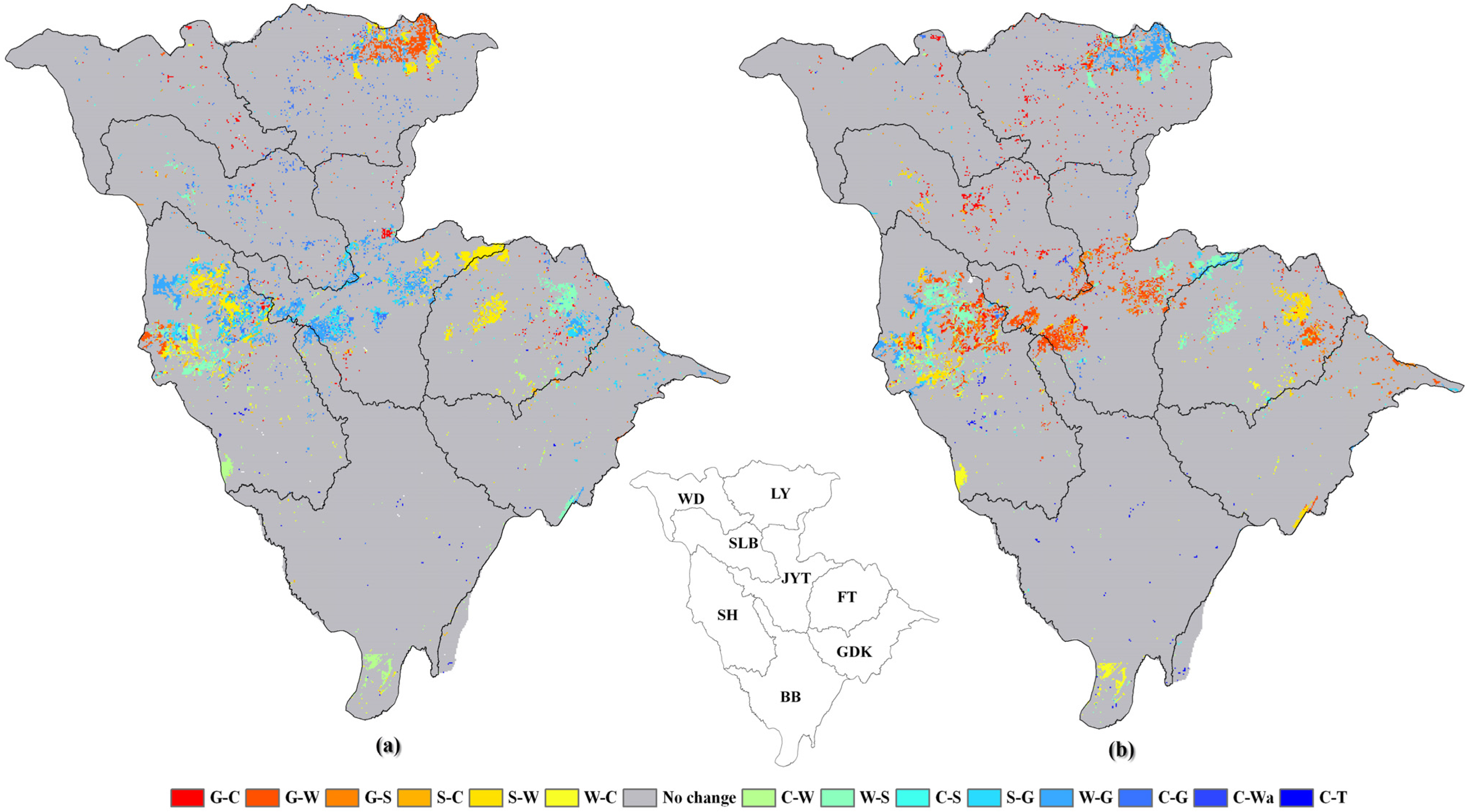
To reflect the dynamic character of spatial land use changes during a specific period, an in-and-out phenomenon is described in Section 3.1. If only the final change is used in the analysis, the real change will be hidden in the process of land use change. For example, this study found that the woodland area in the Jialing River Basin was 31,670 km2 in the 1980s (land use 1985) and 32,193 km2 in the 1990s (land use 1995), which resulted in a final change of 523 km2 (Table 2). From 1985 to 1995, 3894 km2 of woodlands were converted into other land use types, and 3371 km2 of other types of land use were converted to woodland (Table 3). Therefore, the actual change related to woodlands (real change) was up to 7265 km2. In this paper, both the change rate and the change in the area of woodlands were highlighted. This in-and-out phenomenon directly affected the detectability of changes in the hydrological regimes that were caused by land use changes, because the changes in the hydrological elements were normally expressed as an overall value for a catchment or a statistical unit in which the in-and-out phenomenon existed.
From the analysis in Section 3.1, it is clear that the land use along the Jialing River significantly changed. The forces driving the frequent transfer and conversion primarily included economic, population and macro-policy forces. In pursuit of economic development, humans have engaged in extensive land use changes, including building and grazing. These changes have resulted in reduced croplands and the degradation of grasslands, which have resulted in environmental deterioration, but also in changes in land use type. In addition, farmers have adjusted the structure of agricultural production to increase their income, and more young people in rural areas have sought better jobs in large cities. All of these factors have indirectly affected land use patterns. Since 1980, the rapid economic development of the Jialing River has accelerated the urbanization process, which has resulted in the conversion of cropland to other types of land use and has resulted in a greater amount of land under construction. Population is an important factor that could lead to land use change. A population increase results in greater residential land. From the 1980s to 2000, the area of settlement in the Jialing River Basin increased steadily from 313 km² in the 1980s to 378 km² in 1995 and to 489 km² in 2000. However, additional croplands are required to feed the growing population. Since 1985, due to the continuing population growth in the Jialing River Basin (43.9 million in 1995, 44.8 million in 2000, calculated from 1 km × 1 km grid datasets of population, China), industrial development and the expansion of farming areas inevitably resulted in decreasing woodland and grassland areas. Population pressure and human activities are the main reasons for the dramatic changes in the woodland area. In addition, macro-policy is a factor that cannot be neglected. In the 1980s, the government of the P.R. of China implemented a policy to construct a huge shelter-forest system upstream of the Yangtze River. This project was called the “Yangtze River Management” project. The affected area was approximately 200,000 km2, covering Sichuang, Yunnan, Guizhou and Hubei provinces, and included the Tuo River, Min River, Jialing River, Wu River and the mainstream of the Three Gorges [48]. Since the 1990s, a national policy of returning cropland to woodlands and grasslands (RCFG) has been implemented. Furthermore, maintaining a dynamic balance of arable land is currently a basic land use policy in China. All of these factors contributed to dynamic changes in land use within the Jialing River Watershed.

4.2. Hydrological Response

In LY, woodlands increased by 944 km2 (croplands, shrublands and grasslands decreased by 193 km2, 452 km2 and 303 km2, respectively) from 1985 to 1995. In addition, from 1995 to 2000, 936 km2 of woodlands were converted into croplands, shrublands and grasslands, which increased by 216 km2, 453 km2 and 267 km2, respectively. As the woodland area increased, the ET decreased (S1-S0) and vice versa (Table 9). In terms of the hydrological effects of the woodlands, many researchers [3,4,7] have concluded that harvesting forests or converting them into grasslands or croplands decreases the ET because the canopy interception decreases. However, we observed an increase in the ET in this study. Actually, the effects of land use change on hydrological processes are extremely complex. In addition to the biophysical characteristics of vegetation, such as LAI, albedo, stoma resistance and root distribution, differences in the background climate are also important. Actual ET is similar to potential ET for the humid climate characteristic of the upstream region of the Yangtze River [49]. In addition, the lower temperature, higher moisture and slower air exchange in woodlands will decrease ET [48]. Therefore, a decrease in forestland and shrubland may not result in a decrease in ET. The research institute of the Yangtze River Basin’s planning office has observed the same results in their study of paired subcatchments [49]. Furthermore, a study by Zheng et al. [50] of the Pingtong River, one of the subcatchments in the Jialing River, has supported this conclusion.
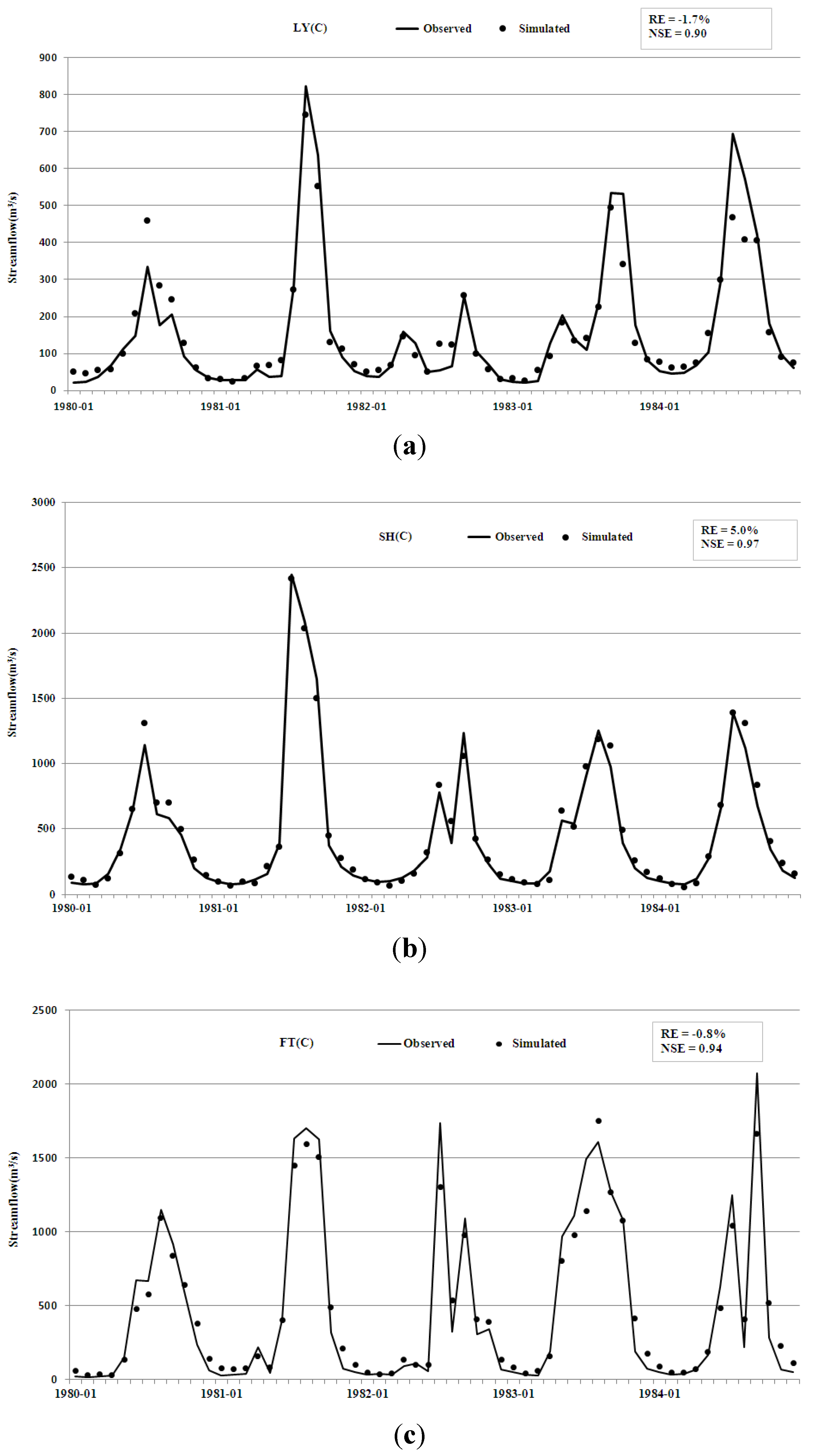
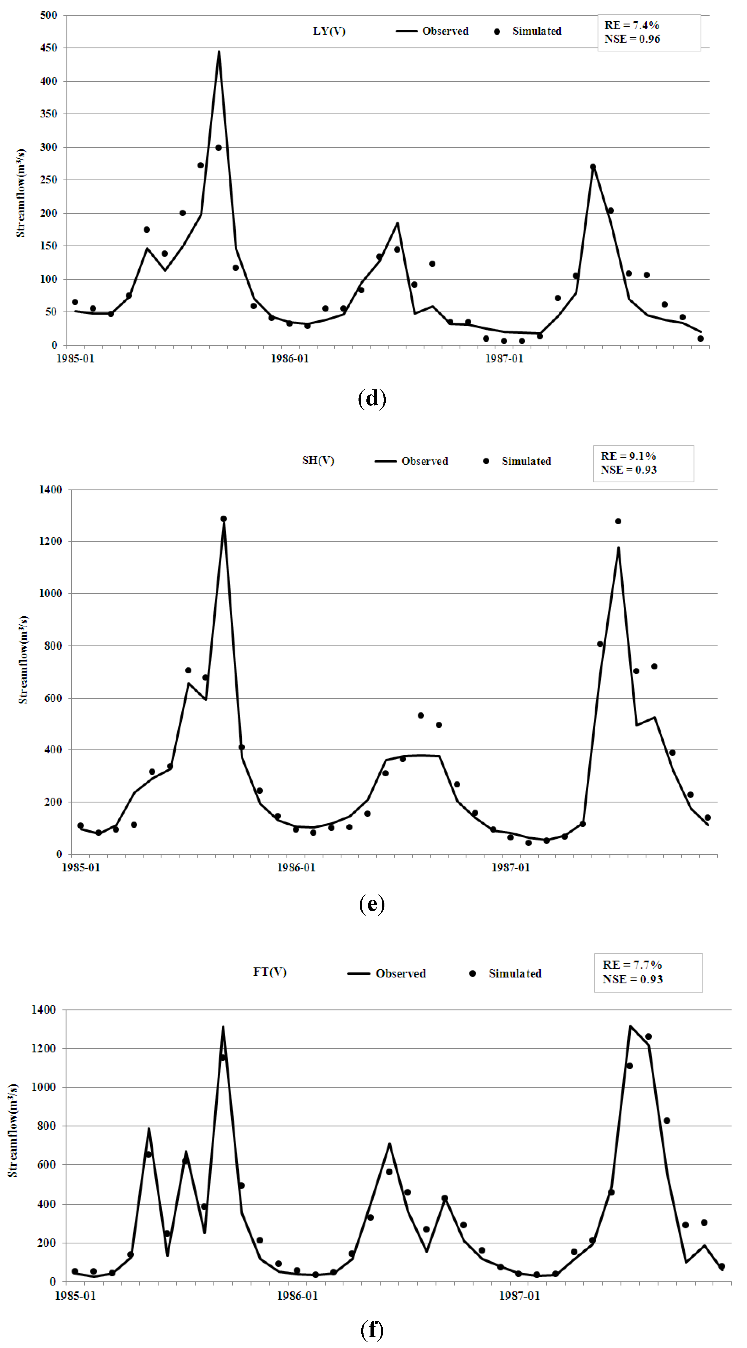
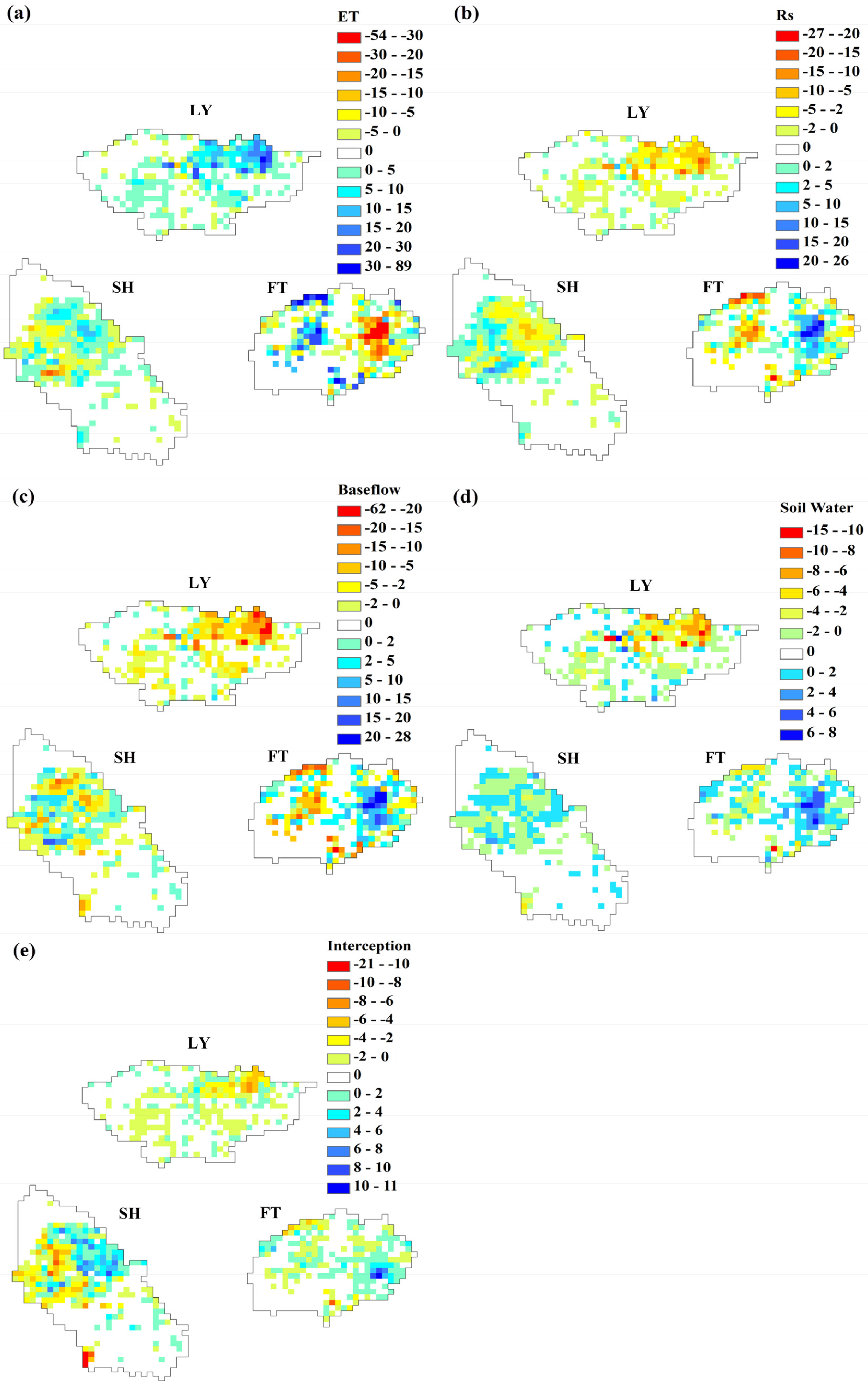
In Scenarios S1-S0 and S2-S1, the hydrological regimes did not change noticeably, as we previously mentioned. However, the land use changed extensively. Lahmer et al. [51] applied a GIS-based modeling approach to two river basins and concluded that moderate land use change results in only small changes in various water balance components. Lu Zhixiang et al. [52] also did not detect obvious changes in hydrological elements, even in two of their three studied subcatchments, where land use changed significantly. Take Subcatchment 7 in their study, for example: from 1995 to 2000, the area of cropland decreased 26.94%, while woodland and grassland area increased 8.69% and 18.55%. Land use changes during this period only led to a 0.47- and 1.64-mm increase in ET and water yield and a 2.37-mm decrease in soil water. Thus, the current paper attempts to explain why this change occurred by combining the concepts of real change and final change with the spatial distribution maps (Figure 4 and Figure 5) and statistic distribution tables of the hydrological elements (Table 11, Table 12, Table 13, Table 14 and Table 15).
Table 11. Statistic distribution of ET variation in Scenario S1-S0 (area percentage, %).
ET−89–−30−30–−20−20–−15−15–−10−10–−5−5–000–55–1010–1515–2020–3030–59
LY0.21.61.83.76.522.654.38.90.20.2000
SH00.20.32.46.922.753.012.70.90.70.200
FT2.22.52.24.24.710.644.212.36.14.92.02.22.0
Table 12. Statistic distribution of Rs variation in Scenario S1-S0 (area percentage, %).
Rs−27–−20−20–−15−15–−10−10–−5−5–−2−2–000–22–55–1010–1515–2020–26
LY0000.20.49.154.521.38.14.51.40.40
SH000.20.91.711.456.116.910.32.40.200
FT0.51.51.04.4 7.612.045.511.17.65.21.50.51.7
Table 13. Statistic distribution of baseflow variation in Scenario S1-S0 (area percentage, %).
Baseflow−31–−20−20–−15−15–−10−10–−5−5–−2−2–000–22–55–1010–1515–2020–62
LY0000.21.08.154.518.710.45.91.2 00
SH000.20.72.113.952.818.27.94.1000
FT1.21.52.07.910.86.444.55.28.17.12.72.00.7
Table 14. Statistic distribution of soil water variation in Scenario S1-S0 (area percentage, %).
Soil water−9–−8−8–−6−6–−4−4–−2−2–000–22–44–66–99–15
LY00.20.20.88.154.519.56.55.73.90.6
SH0000.315.757.325.11.40.200
FT0.20.22.25.721.144.517.46.42.00.00.2
Table 15. Statistic distribution of interception variation in Scenario S1-S0 (area percentage, %).
Interception−12–−10−10–−8−8–−6−6–−4−4–−2−2–000–22–44–66–88–1010–21
LY00000.214.255.924.03.02.20.400
SH0.30.72.92.97.115.052.811.04.31.70.30.30.5
FT0.20.20.50.72.528.747.218.90.7000.20
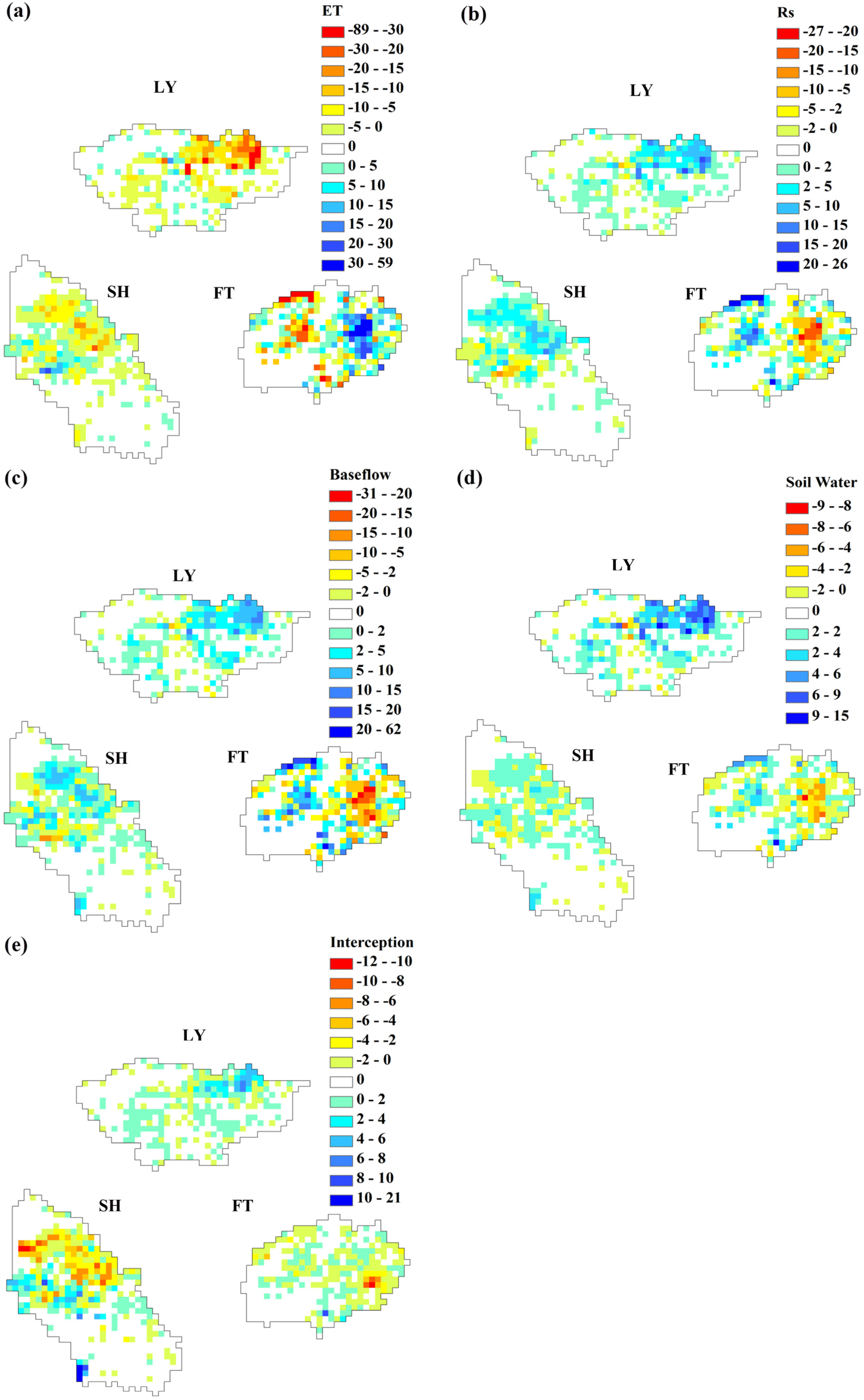
Change in the hydrological elements in S1-S0 can be used as an example, because in this scenario, the hydrological element changed the most. In Figure 4, we can see that the local hydrological elements changed significantly. ET changed from −89 to 59 mm. The generation of surface water changed from −27 to 26 mm. The baseflow changed from −31 to 62 mm, and the soil water and interception changed from −9 to 15 mm and from −12 to 21 mm, respectively. However, the magnitudes of change in the hydrological components in each subcatchment (LY, SH and FT) were not obvious (Table 9). This finding may be explained by the compensation and average effects.
In LY, the difference between the final change and the real change in the hydrological elements was not great (Table 9 and Table 10), which indicated that compensation effect was not obvious. This outcome resulted from the unique directions of change in LY (Figure 4 and Table 11, Table 12, Table 13, Table 14 and Table 15). There were 36.4% of the grids with decreased ET values. Only in 9.3% of area did ET increase. However, other elements have the opposite variation characteristics. Rs, baseflow, soil water content and interception increased in 35.8%, 36.2%, 36.2% and 29.7% and decreased in 9.8%, 9.3%, 9.3% and 14.4% of the area, separately. Thus, the compensation effect of each element was small. Meanwhile, because many grids exhibited no change (around 54.5% of grids) or small change (ET: 22.6% of grids with a range of [−5–0); Rs: 29.4% of grids with a range of (0–5]; baseflow: 29.1% of grids with a range of (0–5]; soil water content: 31.7% of grids with a range of (0–6]; and interception: 29.3% of grids with a range of (0–6]), the average effect was great. Essentially, little overall change occurred in the hydrological regimes in LY.
SH and FT had more significant real changes than LY. In the SH and FT, positive and negative changes occurred in each element (Figure 4 and Table 11, Table 12, Table 13, Table 14 and Table 15). The compensation effect played an important role that made it difficult to detect the change. The FT showed the largest difference between real change and final change (Table 9 and Table 10). In FT, there was 26.3% of the area with decreased ET and 29.5% with increased ET. The proportions of area for other hydrological components (Rs, baseflow, soil water content and interception) with decreased values were 27.0%, 29.7%, 29.5% and 32.9%, separately. Correspondingly, the area percentages with increased values were 29.5%, 27.5%, 25.8%, 26.0% and 19.9%. The increased area and decreased area were similar. This made it difficult to detect variations that result from land use changes in the hydrological elements.
To detect obvious changes in hydrological components caused by land use change, it is necessary to pay attention to the scale problem. In a large watershed, the compensation and average effects may decrease the detectability.

5. Conclusions

Based on the analysis above, we reached the following three conclusions:
(1)
The land use quantities and spatial configuration in the Jialing River Basin changed dramatically due to economic development, population growth and national macro-policy. Settlement and shrubland areas changed significantly, with final change rates of 20.77% and −16.07%, respectively, from 1985 to 1995; real change rates of 34.2% and 30.1%, respectively, from 1985 to 1995; final change rates of 29.37% and 12.40%, respectively, from 1995 to 2000; and real change rates of 39.9% and 32.8%, respectively, from 1995 to 2000. Due to an in-and-out conversion relationship, the actual land use change was hidden in the final change analysis. In the real change analysis, the change rate and change in woodland area were highlighted. These changes were more dynamic in the LY, SH and FT subcatchments;
(2)
The decrease in woodland area in the LY subcatchment resulted in greater ET; however, the other hydrological elements decreased;
(3)
Although the hydrological elements changed little overall due to the average and compensation effects, they changed significantly at the local scale. Real change analysis can reduce the compensation effects and enhance the detectability of change.
This study considered the concepts of real change and final change and the average and compensation effects, which are important for deeply analyzing land use changes and their impacts on hydrological regimes.

Acknowledgments

The study is supported by the National Natural Science Foundation of China (41030636), the National High Technology Research and Development Program of China (2012AA12A309), National Natural Science Foundation of China (51420105014) and the Research and Innovation Project for College Graduates of Jiangsu Province (CXZZ12_0239).

Author Contributions

All authors contributed to the design and development of this manuscript. Tao Zhang carried out the statistical analysis of results and prepared the first draft of the manuscript; Xingnan Zhang as the supervisor of Tao Zhang provided many important advices on the concept of methodology and structure of the manuscript, as well as edited the manuscript during revisions; Dazhong Xia was responsible for the land use change analysis part of the paper; Yangyang Liu constructed VIC model in study area.

Conflicts of Interest

The authors declare no conflict of interest.

References

  1. Zhang, L.T.; Ding, W.R.; Zhou, Y.; Zhang, L. Study on land use and land cover change. Environ. Sci. Surv. 2007, 26, 7–10. [Google Scholar]
  2. Chen, J.; Li, X. Simulation of hydrological response to land-cover changes. Chin. J. Appl. Ecol. 2004, 15, 833–836. [Google Scholar]
  3. Dunn, S.M.; Mackay, R. Spatial variation in evapotranspiration and the influence of land use on catchment hydrology. J. Hydrol. 1995, 1995, 49–73. [Google Scholar] [CrossRef]
  4. Matheussen, B.; Krichbaum, R.L.; Goodman, I.A.; O’Donnell, G.M.; Lettenmaier, D.P. Effects of land cover change on streamflow in the interior Columbia River Basin. Hydrol. Process. 2000, 14, 867–885. [Google Scholar] [CrossRef]
  5. Olchev, A.; Ibrom, A.; Priess, J.; Erasmi, S.; Leemhuis, C.; Twele, A.; Radler, K.; Kreilein, H.; Panferov, O.; Gravenhorst, G. Effects of land-use changes on evapotranspiration of tropical rain forest margin area in Central Sulawesi (Indonesia): Modelling study with a regional SVAT model. Ecol. Model. 2008, 212, 131–137. [Google Scholar] [CrossRef]
  6. Jin, C.; Zhang, B.; Song, K.; Wang, Z.; Yang, G. RS-based analysis on the effects of land use/cover change on regional evapotranspiration: A case study in Qian’an County, Jilin Province. Arid Zone Res. 2009, 26, 734–743. [Google Scholar] [CrossRef]
  7. Mao, D.Z.; Cherkauer, K.A. Impacts of land-use change on hydrologic responses in the Great Lakes region. J. Hydrol. 2009, 374, 71–82. [Google Scholar] [CrossRef]
  8. Andraski, B.J. Soil-water movement under natural-site and waste-site conditions: A multiple-year field study in the Mojave Desert, Nevada. Water Resour. Res. 1997, 33, 1901–1916. [Google Scholar] [CrossRef]
  9. Shi, P.L.; Li, W.H. Influence of forest cover change on hydrological process and watered runoff. J. Nat. Resour. 2001, 16, 481–487. [Google Scholar]
  10. Krause, P. Quantifying the impact of land use changes on the water balance of large catchments using the J2000 model. Phys. Chem. Earth 2002, 27, 663–673. [Google Scholar] [CrossRef]
  11. Legesse, D.; Vallet-Coulomb, C.; Gasse, F. Hydrological response of a catchment to climate and land use changes in Tropical Africa: case study South Central Ethiopia. J. Hydrol. 2003, 275, 67–85. [Google Scholar] [CrossRef]
  12. Coe, M.T.; Costa, M.H.; Soares-Filhoc, B.S. The influence of historical and potential future deforestation on the stream flow of the Amazon River—Land surface processes and atmospheric feedbacks. J. Hydrol. 2009, 369, 165–174. [Google Scholar] [CrossRef]
  13. Savary, S.; Rousseau, A.N.; Quilbe, R. Assessing the effects of historical land cover changes on runoff and low flows using remote sensing and hydrological modeling. J. Hydrol. Eng. 2009, 14, 575–587. [Google Scholar] [CrossRef]
  14. Schilling, K.E.; Chan, K.S.; Liu, H.; Zhang, Y.K. Quantifying the effect of land use land cover change on increasing discharge in the Upper Mississippi River. J. Hydrol. 2010, 387, 343–345. [Google Scholar] [CrossRef]
  15. Storck, P.; Bowling, L.; Wetherbee, P.; Lettenmaier, D. Application of a GIS-based distributed hydrology model for prediction of forest harvest effects on peak stream flow in the Pacific Northwes. Hydrol. Process. 1998, 12, 889–904. [Google Scholar] [CrossRef]
  16. Fohrer, N.; Haverkamp, S.; Eckhardt, K.; Frede, H.G. Hydrologic response to land use changes on the catchment scale. Phys. Chem. Earth Part B Hydrol. Oceans Atmos. 2001, 26, 577–582. [Google Scholar] [CrossRef]
  17. Sun, H.N. Progress of research on the role of forest during past 20 years. J. Nat. Resour. 2001, 16, 407–412. [Google Scholar]
  18. Hundecha, Y.; Bardossy, A. Modeling of the effect of land use changes on the runoff generation of a river basin through parameter regionalization of a watershed model. J. Hydrol. 2004, 292, 281–295. [Google Scholar] [CrossRef]
  19. Archer, D.R.; Climent-Soler, D.; Holman, I.P. Changes in discharge rise and fall rates applied to impact assessment of catchment land use. Hydrol. Res. 2010, 41, 13–26. [Google Scholar] [CrossRef]
  20. Cuo, L.; Lettenmaier, D.P.; Alberti, M.; Richey, J.E. Effects of a century of land cover and climate change on the hydrology of the Puget Sound basin. Hydrol. Process 2009, 23, 907–933. [Google Scholar] [CrossRef]
  21. Liu, Y.; Zhang, X.; Xia, D.; You, J.; Rong, Y.; Bakir, M. Impacts of land-use and climate changes on hydrologic processes in the Qingyi River watershed, China. J. Hydrol. Eng. 2013, 18, 1495–1512. [Google Scholar] [CrossRef]
  22. Ghaffari, G.; Keesstra, S.; Ghodousi, J.; Ahmadi, H. SWAT-simulated hydrological impact of land-use change in the Zanjanrood basin, Northwest Iran. Hydrol. Process 2010, 24, 892–903. [Google Scholar] [CrossRef]
  23. Ashagrie, A.G.; de Laat, P.; de Wit, M.; Tu, M.; Uhlenbrook, S. Detecting the influence of land use changes on discharges and floods in the Meuse River Basin—The predictive power of a ninety-year rainfall-runoff relation? Hydrol. Earth Syst. Sci. 2006, 10, 691–701. [Google Scholar] [CrossRef]
  24. Xian, W.; Shao, H.Y.; Zhou, W.C. The dynamic monitoring and prediction of land use pattern in the area of middle and lower reaches of the Jialingjiang River. Res. Soil Water Conserv. 2005, 12, 61–64. [Google Scholar]
  25. Tang, Q.; Shao, H.; Xian, W.; Zhou, W. Dynamic change in land use/cover in middle and lower reaches of the Jialing River. Soils 2006, 38, 36–41. [Google Scholar]
  26. Shao, H.; Xian, W.; Yang, W. Contrastive research on the process of land use change in main valleys of the upper reaches of the Yangtze River. Ecol. Environ. 2008, 17, 792–797. [Google Scholar]
  27. Wu, X.; Shen, Z.; Liu, R. Study on the reginal differntation of land use/land cover change in the upper reaches of Yangtze River. J. Basic Sci. Eng. 2008, 16, 819–829. [Google Scholar]
  28. Leng, S.; Zhang, X.; Xia, D.; Liu, Y. Dynamic analysis of landscape structure of land use in Jialingjiang Watershed. J. China Three Gorge Univ. Nat. Sci. 2012, 34, 38–42. [Google Scholar]
  29. Qi, S.; Zhang, X.; Xia, D.; Liu, Y.; Liu, B. Characteristic and driving forces of land use/cover change in Jialingjiang River Basin. J. Yangtze River Sci. Res. Inst. 2013, 30, 1–7. [Google Scholar]
  30. Data Center for  Resources and Environmental Sciences, Chinese Academy of Sciences (RESDC). Available online: http://www.resdc.cn (accessed on 19 June 2013). (In Chinese)
  31. Zhang, X.N.; Liu, Y.Y.; Fang, Y.H.; Liu, B.J.; Xia, D.Z. Modeling and assessing hydrologic processes for historical and potential land-cover change in the Duoyingping watershed, southwest China. Phys. Chem. Earth 2012, 53–54, 19–29. [Google Scholar] [CrossRef]
  32. Shuttle Radar Topography Mission (SRTM) Website. Available online: http://srtm.csi.cgiar.org/ (accessed on 1 September 2012).
  33. Reynolds, C.A.; Jackson, T.J.; Rawls, W.J. Estimating available water content by linking the FAO soil map of the world with global soil profile databases and pedo-transfer functions. In Proceedings of the AGU 1999 Spring Conference, Boston, MA, USA, 1–4 June 1999.
  34. Lin, Q.; Luo, G.P.; Chen, X. Review of land use model. Prog. Geogr. 2005, 24, 81–89. [Google Scholar]
  35. Wang, X.L.; Bao, Y.H. Study on the methods of land use dynamic change research. Prog. Geogr. 1999, 18, 83–89. [Google Scholar]
  36. Zhu, H.Y.; Li, X.B. Discussion on the index method of redional land use change. J. Geogr. Sci. 2003, 58, 643–650. [Google Scholar]
  37. Liu, Y. Characteristics of Land Cover Change and Hydrologic Responses at the Watershed Scale. Ph.D. Thesis, Hohai University, Nanjing, China, 31 May 2012. [Google Scholar]
  38. Liang, X.; Lettenmaier, D.P. A simple hydrologically based model of land surface water and energy fluxes for general circulation models. J. Geophys. Res. 1994, 99, 14415–14428. [Google Scholar] [CrossRef]
  39. Liang, X.; Wood, E.F.; Lettenmaier, D.P. Surface soil moisture parameterization of the VIC-2L model: Evaluation and modification. Glob. Planet. Change 1996, 13, 195–206. [Google Scholar] [CrossRef]
  40. Nijssen, B.; Lettenmaier, D.P.; Liang, X.; Wetzel, S.W.; Wood, E.F. Streamflow simulation for continental-scale river basins. Water Resour. Res. 1997, 33, 711–724. [Google Scholar] [CrossRef]
  41. Gao, H.; Tang, Q.; Shi, X.; Zhu, C.; Bohn, T.; Su, F.; Sheffield, J.; Pan, M.; Lettenmaier, D.; Wood, E.F. Water Budget Record from Variable Infiltration Capacity (VIC) Model. http://www.hydro.washington.edu/Lettenmaier/Models/VIC/Documentation/References.shtml (accessed on 13 March 2013).
  42. VanShaar, J.; Haddeland, I.; Lettenmaier, D.P. Effects of land-cover changes on the hydrological response of interior Columbia River basin forested catchments. Hydrol. Process 2002, 12, 2499–2520. [Google Scholar] [CrossRef]
  43. Hurkmans, R.T.W.L.; Terink, W.; Uijlenhoet, R.; Moors, E.J.; Troch, P.A.; Verburg, P.H. Effects of land use changes on streamflow generation in the Rhine basin. Water Resour. Res. 2009, 45, 1–15. [Google Scholar]
  44. Mishra, V.; Cherkauer, K.A.; Niyogi, D.; Lei, M.; Pijanowski, B.C.; Ray, D.K.; Bowling, L.C.; Yang, G. A regional scale assessment of land use/land cover and climatic changes on water and energy cycle in the upper Midwest United States. Int. J. Climatol. 2010, 30, 2025–2044. [Google Scholar] [CrossRef]
  45. Cuo, L.; Zhang, Y.; Gao, Y.; Hao, Z.; Cairang, L. The impacts of climate change and land cover/use transition on the hydrology in the upper Yellow River Basin, China. J. Hydrol. 2013, 502, 37–52. [Google Scholar] [CrossRef]
  46. Nash, J.E.; Sutcliffe, J.V. River flow forecasting through conceptual models part I—A discussion of principles. J. Hydrol. 1970, 10, 282–290. [Google Scholar] [CrossRef]
  47. ArcGIS for Desktop. Available online: http://www.esri.com/software/arcgis/arcgis-for-desktop (accessed on 12 October 2009).
  48. Cheng, G.W.; Sun, Y. Forest change: Hydrological effects in the upper Yangtze River Valley. Ambio 1999, 28, 457–459. [Google Scholar]
  49. Liu, C.M.; Chung, C.H. The influence of forest cover upon annal runoff in the loess plateau of China. J. Geogr. Sci. 1978, 33, 112–127. [Google Scholar]
  50. Zheng, S.; Mu, C.; Chen, Z.; Gong, G.; Li, Y. Simulations and analysis on the effects of forest on the hydrological process in the upper reaches of Yangtze River. Acta Ecol. Sinica 2010, 30, 3046–3056. [Google Scholar]
  51. Lahmer, W.; Pfützner, B.; Becker, A. Assessment of land use and climate change impacts on the mesoscale. Phys. Chem. Earth Part. B Hydrol. Oceans Atmos. 2001, 26, 565–575. [Google Scholar] [CrossRef]
  52. Lu, Z.X. A study of the land use change and its hydrologic response in the upper reaches of the Fen River. J. Glaciol. Geocryol. 2014, 36, 192–199. [Google Scholar]

