3.1. Assessing the Relationship between Rainfall and Stream Flow
The open source software R [
33] was used for the analyses in this paper. We calculate 10 subseries of rainfall and stream flow from 1990 to 2012 using the “wavethresh” R routine packages [
34,
35] for assessing the relationship between rainfall and stream flow. The length of time taken into account in 10 subseries for rainfall and stream flow is a period of 512 days.
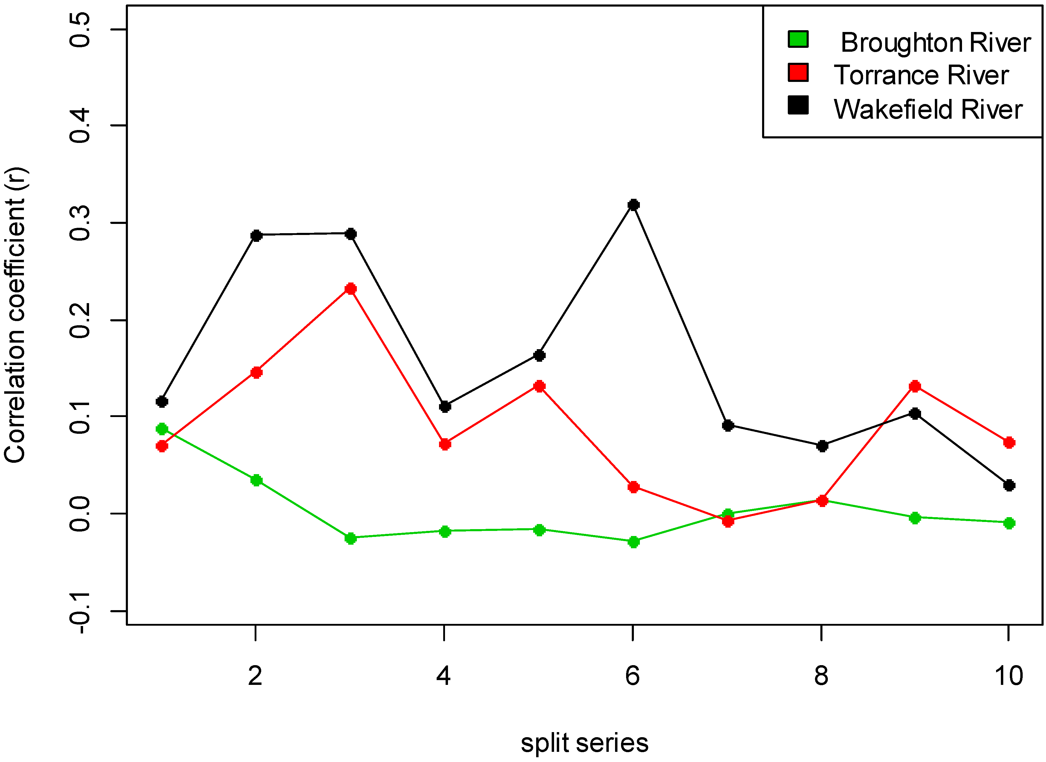
The relationship between rainfall and stream flow within 10 subseries is presented in
Figure 2. The maximum correlation coefficients are 0.08, 0.23 and 0.31 at Broughton River, Torrance River and Wakefield River, respectively. These values are between −1 and +1 in all cases, indicating the degree of linear dependence between rainfall and stream flow. For assessing short term spatial variability, a correlation coefficient of the sub-series of rainfall and stream flow less than 0.4 indicates a significant difference from 0 at each station. For example, in sub-series 2, the correlation coefficient was 0.04, 0.15 and 0.28 which indicates the independence of rainfall and stream flow at Broughton River, Torrance River and Wakefield River, respectively.
Figure 2.
Correlation pattern subseries of rainfall and stream flow time series.
Figure 2.
Correlation pattern subseries of rainfall and stream flow time series.
In order to understand stream flow availability under the climatic conditions in South Australia, we investigated the characteristics of rainfall and stream flow patterns, as categorized by climatic phenomena. A statistical measure of the dispersion of rainfall and stream flow patterns around the mean is defined as follows:
where
CV is defined as the coefficient of variation and is represented by the ratio of the standard deviation (
Sx) to the mean (
µx).
Table 2 shows the degree of variation in rainfall and stream flow patterns.
Table 2.
Rainfall and stream flow variability at Broughton River, Torrance River and Wakefield River in South Australia (SA) from 1990 to 2011.
Table 2.
Rainfall and stream flow variability at Broughton River, Torrance River and Wakefield River in South Australia (SA) from 1990 to 2011.
| Statistics | Broughton River | Torrance River | Wakefield River |
|---|
| Rainfall | Stream flow | Rainfall | Stream flow | Rainfall | Stream flow |
|---|
| Mean | 1.653 | 9.817 | 1.530 | 5.396 | 1.282 | 25.333 |
| Estimated standard deviation | 0.385 | 4.075 | 0.296 | 4.201 | 0.223 | 21.300 |
| Coefficient of variation (CV) | 23.31% | 41.51% | 19.36% | 77.85% | 17.40% | 84.07% |
In
Table 2, the CV for stream flow patterns indicates higher variability than for the rainfall series.
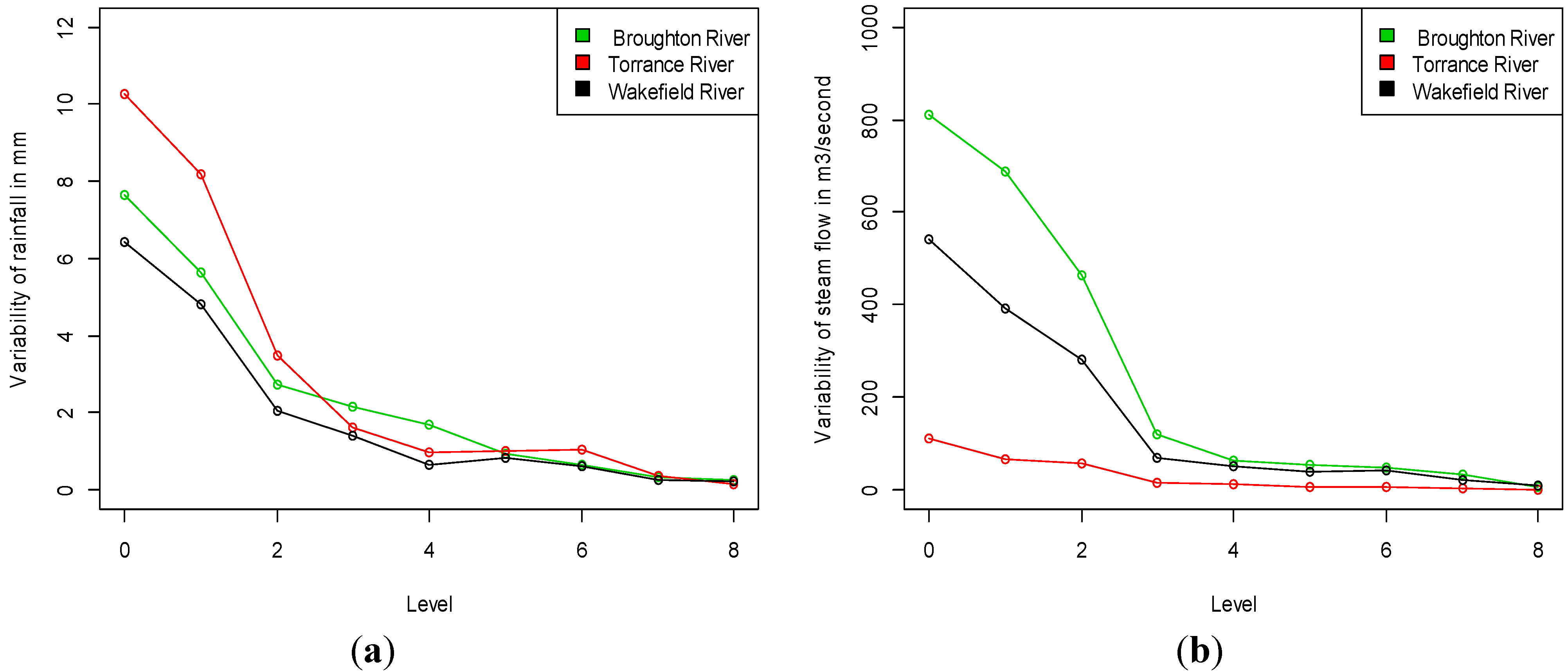
Figure 3 shows the variability of the wavelet coefficients from levels 0 to 8. The evidence of association between the rainfall and stream flow coefficient is strongly correlated at the 5% significance level in
Table 1.
Figure 3.
Standard deviations of wavelet coefficients of rainfall and stream flow from level 0 to 8. (a) Rainfall; (b) Stream flow.
Figure 3.
Standard deviations of wavelet coefficients of rainfall and stream flow from level 0 to 8. (a) Rainfall; (b) Stream flow.
3.2. Correlation Structures between Rainfall and Stream Flow
In the previous sections, we calculated wavelet coefficients for each subset of the rainfall and stream flow series. In order to filter each of those series, we applied Haar wavelets.
The constructed correlation pattern for each rainfall and stream flow sub-series for levels 0 to 8 is given by:
and
where
rk is the constructed correlation with level n from 0 to 8 and
is the
jth sub-series of the rainfall and stream flow wavelet decomposed with the Haar procedure. The results are presented in
Table 3.
The evidence of significant correlation (
r ≥ 0.50) between rainfall and stream flow wavelet coefficient series with at least a 5% significance level is shown in
Table 3. Furthermore, to avoid co-linearity problems, the squared rainfall and stream flow wavelet coefficient series are also included. We found that a correlation structure (
r = 0.56) such as stream flow is determined by rainfall on at least 4 days with 5% level at the Broughton River Basin and Torrance River Basin, as shown in
Table 3. The adjusted squared stream flow and rainfall has a little evidence of correlations (
i.e., at 5% level) up to 64 days at Torrance River at, also a marginal correlation (
r = 0.51) up to 128 days within squared adjusted rainfall and adjusted stream flow at Wakefield River. The rainfall and stream flow relationship was used to develop a response model for predicting stream flow.
Table 3.
Constructed correlation pattern for different levels between (a) adjusted rainfall and adjusted stream flow; (b) squared adjusted rainfall and adjusted stream flow; (c) adjusted rainfall and squared adjusted stream flow; (d) squared adjusted rainfall and squared adjusted stream flow.
Table 3.
Constructed correlation pattern for different levels between (a) adjusted rainfall and adjusted stream flow; (b) squared adjusted rainfall and adjusted stream flow; (c) adjusted rainfall and squared adjusted stream flow; (d) squared adjusted rainfall and squared adjusted stream flow.
| Days | Broughton River | Torrance River | Wakefield River |
|---|
| a | b | c | d | a | b | c | d | a | b | c | d |
|---|
| 1 | 0.71 ** | 0.89 *** | 0.70 ** | 0.86 *** | 0.76 ** | −0.184 | −0.513 | 0.447 | 0.76 ** | −0.53 * | −0.59 * | 0.86 *** |
| 2 | 0.65 * | 0.264 | 0.469 | 0.449 | 0.72 ** | 0.57 | 0.158 | 0.265 | 0.384 | 0.413 | 0.201 | 0.038 |
| 4 | 0.56 * | −0.189 | 0.257 | 0.146 | 0.63 * | 0.061 | −0.27 | 0.125 | 0.324 | −0.28 | −0.341 | 0.115 |
| 8 | 0.087 | 0.369 | −0.296 | 0.103 | 0.032 | 0.55 * | 0.173 | −0.51 * | −0.369 | 0.483 | 0.191 | −0.418 |
| 16 | 0.233 | 0.08 | −0.009 | −0.326 | 0.275 | −0.15 | 0.009 | −0.311 | 0.306 | −0.652 | 0.081 | −0.393 |
| 32 | 0.094 | 0.055 | −0.059 | −0.248 | 0.68 * | −0.84 ** | −0.81 *** | 0.97 *** | −0.116 | 0.002 | −0.382 | −0.121 |
| 64 | 0.411 | 0.036 | 0.292 | 0.238 | 0.488 | 0.67 * | 0.456 | 0.71 ** | −0.091 | 0.166 | −0.005 | −0.301 |
| 128 | 0.423 | −0.409 | 0.604 * | 0.68 * | 0.299 | −0.162 | 0.186 | −0.223 | 0.279 | −0.575 | 0.128 | −0.51 * |
| 512 | 0.456 | 0.354 | −0.292 | 0.343 | −0.218 | −0.405 | 0.007 | −0.405 | 0.094 | 0.117 | 0.098 | −0.163 |
3.3. Rainfall-Stream Flow Response Modeling
The constructed correlations described in the previous section may be partly due to common seasonal variations and trends, so a first step is to estimate these deterministic features with regression models for entire period from 1990 to 2010. The residuals from these regressions are reformed to the deseasonalized and detrended (dsdt) time series. For all three stations, a cubic trend gave a statistically improved fit over a linear or quadratic trend over the study period. The seasonal variation was reasonably modelled by a sinusoidal curve. Therefore, the regression models are of the form:
where,
Ti represents either rainfall or stream flow; time is the mean adjusted time, that is
where
t is the number of days from the start of the record and
is the mean of
t,
time2 and
time3, which allows for possible quadratic and cubic trends;
C is cos(2πt/365.25) and
S is sin(2πt/365.25) and together these allow for seasonal variation of period one cycle per year;
βj are the unknown coefficients to be estimated; and
εt are random variations with mean 0 and constant standard derivation.
For the estimated coefficients, only a few values are significantly different from 0 even at the 5% significance level, as shown in
Table 4. There is evidence of significantly different trends in rainfall at Wakefield River, which may have corresponded to increased stream flows if rainfall is increased. We have predicted the stream flow (
Yt) on day
t from rainfall (
Xt) with corresponding lags
k. This is referred to as a Response Model (RM). The regression is defined as:
We assess stream flow in response to rainfall at lags 0 to 128. The best fitted model is selected based on the adjusted coefficient of determination;
; minimum sigma squared (
σ2) and the Akaike Criterion Information (AIC); The AIC is defined as:
where L is the maximized value of the likelihood function for the estimated model. Comparisons of the AIC for different model is as shown in
Table 5. The
value significantly reduces and the estimated stream flow influence is close to zero after the exogenous rainfall at lag 7. Therefore, we reduced the exogenous rainfall at lags from 128 to 7 in the response model; referred to as RM0 in
Table 5. This strategy is sub-optimal inasmuch as rejected terms might meet the retention criterion if added back individually. However; any small improvement in
would be balanced by increased complexity in the model; which is undesirable if interaction and squared terms are added. The regression model is defined as RM:
In the second model, we add deterministic features to the regression model including linear, quadratic and cubic terms of
t, allowing for seasonality effects. This model is defined as RM_D:
where
.
The third model is defined as RMD_AR[1] and is an autoregressive model of order 1 (AR[1]) with RM_D. It can be written in the form:
The fourth model is defined as RMD_AR[2], and is an autoregressive model of order 2 (AR[2]) with RMD_AR[1]. It can be written in the form:
Table 4.
Estimated coefficients of rainfall and stream flow variability from 1990 to 2012.
Table 4.
Estimated coefficients of rainfall and stream flow variability from 1990 to 2012.
| Station | Statistical Summary | Intercept (β0) | Linear Term t | Quadratic Term t | Cubic Term t |
|---|
| Broughton River | Estimated rainfall | 1.58 | −0.000042 | −0.000000001 | −0.000000000003 |
| Variability of rainfall | 0.106 | 0.00008 | 0.000000017 | 0.000000000008 |
| Estimated stream flow | 52.08 | −0.01244 * | 0.0000031 * | −0.000000000258 |
| Variability of stream flow | 6.18 | 0.004661 | 0.0000009 | 0.000000000485 |
| Torrance River | Estimated rainfall | 1.424 | −0.00007 | 0.000000019 | 0.000000000004 |
| Variability of rainfall | 0.077 | 0.00006 | 0.000000012 | 0.000000000006 |
| Estimated stream flow | 3.47 | −0.00174 * | 0.0000003 * | 0.000000000149 * |
| Variability of stream flow | 0.607 | 0.0004573 | 0.000000092 | 0.000000000048 |
| Wakefield River | Estimated rainfall | 1.226 | −0.000123 * | 0.0000000037 | 0.00000000001 * |
| Variability of rainfall | 0.067 | 0.000051 | 0.00000001 | 0.000000000005 |
| Estimated stream flow | 15.95 | −0.01144 * | 0.0000007 | 0.0000000008 * |
| Variability of stream flow | 3.576 | 0.002694 | 0.0000005 | 0.000000000280 |
Table 5.
Fitted regression model for Broughton River, Torrance River and Wakefield River.
Table 5.
Fitted regression model for Broughton River, Torrance River and Wakefield River.
| Model | Broughton River | Torrance River | Wakefield River |
|---|
| Std. Error | AIC | RMSE * | | Std. Error | AIC | RMSE * | | Std. Error | AIC | RMSE * |
|---|
| RMO | 0.16 | 333.6 | 1104.9 | 3.5107 | 0.24 | 31.19 | 742.77 | 5.074 | 0.13 | 195.8 | 1023.53 | 1.1777 |
| RM_D | 0.18 | 331.3 | 1103.9 | 3.1507 | 0.26 | 31.02 | 741.9 | 5.012 | 0.14 | 195.3 | 1023.1 | 1.1777 |
| RMD_AR[1] | 0.35 | 292.9 | 1085.1 | 0.0353 | 0.42 | 27.35 | 722.7 | 0.052 | 0.21 | 187.4 | 1016.9 | 0.11777 |
| RMD_AR[2] | 0.36 | 291.7 | 1084.5 | 0.0313 | 0.43 | 27.35 | 722.5 | 0.0452 | 0.22 | 187.4 | 1016.8 | 0.10777 |
| RMD_tau | 0.39 | 285.8 | 1081.4 | 0.0035 | 0.42 | 27.32 | 722.1 | 0.0411 | 0.23 | 187.3 | 1016.1 | 0.10178 |
Finally, we develop a model for a benchmark comparison of stream flow on day t based on the entire previous period of stream flow and their influence (
τ) adding with model RM_D. This model is defined as RMD_tau. Tau (
τ) is 0 if there is no stream flow influence from the previous day’s rainfall. We have demonstrated an example of count stream flow influence in
Table 6.
Table 6.
An example of count tau and stream flow influence rainfall over time.
Table 6.
An example of count tau and stream flow influence rainfall over time.
| Stream flow | y1 | y2 | y3 | y4 | y5 | y6 | y7 | y8 | y9 | y10 | y11 | y12 | y13 |
| 8 | 9 | 0 | 0 | 0 | 2 | 9 | 22 | 3 | 5 | 8 | 8 | 6 |
| Rainfall | x1 | x2 | x3 | x4 | x5 | x6 | x7 | x8 | x9 | x10 | x11 | x12 | x13 |
| 3 | 2 | 5 | 3.2 | 3 | 2.8 | 2.6 | 2.4 | 2.2 | 2 | 1.8 | 1.6 | 1.4 |
In the
Table 6, when the day t = 6, Y6 = 2, then we count tau = 3 (number of 0), and Y6-3-1 = 9, can be applied in the referred model RMD_tau.
The model RMD_tau can be written in the form:
The fitted model for predicted stream flow in response to exogenous rainfall, deterministic features of the regression model, and previous stream flow influence, is presented in
Table 5. The best fitting model selection was based on minimum AIC and minimum root mean square Error (RMSE). The RMSE is defined as:
where,
is defined as the estimated stream flow and
Yt is the observed stream flow, respectively.
The response model RM0 has 128 predictor variables namely the rainfall lags at 0 to 128. Therefore, there are 129 parameters to estimate including the intercept. The estimated rainfall effects belong to 0 up to 7 days lag, therefore we reduced the rainfall lags from 128 to 7 days and the optimized
values for this model are 0.16, 0.24 and 0.13 for Broughton River, Torrance River and Wakefield River, respectively, as presented in
Table 5. We also offset the cross product term of lags to further reduce the complexity of this model. The second model included linear quadratic and cubic terms, and this model is denoted as RM_D. The number of parameters to be estimated is therefore 8 + 3 = 11 and the
increased to 0.18, 0.26 and 0.14 for Broughton River, Torrance River and Wakefield River, respectively, which is a practical and statistically significant improvement. We then added a first order autoregressive term, referred to as a RMD_AR[1] model, and a second order autoregressive term referred to as a RMD_AR[2] model. We also made a benchmark comparison by using the entire stream flow record and this model is denoted RMD_tau, as presented in
Table 5.
In
Table 5, there is evidence of improvement of
values, RMSE in m
3s
−1 from RM to RM_D. Adding autoregressive order 1 (AR[1]) with RM_D results in substantially improved
values (from 0.18, 0.26, and 0.14 to 0.35, 0.42 and 0.21 for Broughton River, Torrance River and Wakefield River, respectively. Furthermore, when adding autoregressive order 1 (AR[1]) with RM_D, there is evidence of improvement but this may be offset by the increasing number of parameters that affect the complexity of the model. In addition, the RMD_tau model represents a small improvement for two of the three river basins. The best fitted models are RMD_tau for Broughton River, RMD_AR[2] for Torrance River and RMD_tau for Wakefield River, were selected based on the minimum Akaike Information Criterion (AIC) and minimum root mean square error (RMSE) in m
3s
−1. The residuals from the best fitted models were transformed to normalized form by factor multiplication. A factor was calculated, which allows for the fact that the mean of a non-linear function of a random variable is not equal to that function of the mean. The transform series follow an identically normalized form with mean (
μ) of zero, standard deviation (
σ2) of 1 and a random disturbance term (
εt) which is uncorrelated. The transformed series were used to predict the stream flow on day
t based on the predicted stream flow influence over the short term, as shown in
Figure 4.
Figure 4.
Predicted stream flow based on dsdt rainfall for (a) Broughton River; (b) Torrance River; and (c) Wakefield River from 1990 to 2010.
Figure 4.
Predicted stream flow based on dsdt rainfall for (a) Broughton River; (b) Torrance River; and (c) Wakefield River from 1990 to 2010.
In
Figure 4, we demonstrate the versatility of stream flow prediction. It can be seen that this is a non-linear relationship when expressed in terms of the physical interpretation of stream flow based on rainfall.
3.4. Modeling Stream Flow Using an Artificial Neural Network
Artificial neural network (ANN) techniques are motivated by the principles of biological nervous systems [
36]. Although there are different types of ANN, the multilayer feed forward network is the most commonly used technique. For example, a common approaches of training using back-propagation in a multi-layer feed forward network [
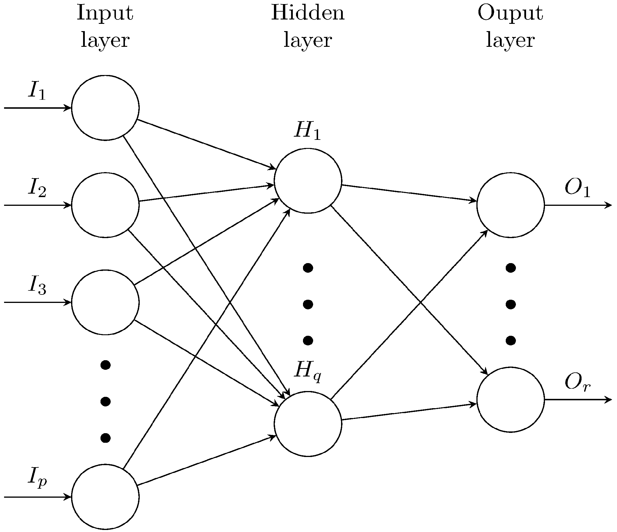
23]. The network consists of input, hidden and output layers. Each layer is fully connected with the proceeding layer with weights in each connection, as shown in
Figure 5.
Figure 5.
A schematic ANN including input, hidden and output layers.
Figure 5.
A schematic ANN including input, hidden and output layers.
In
Figure 5, the number of nodes in the input layer is p, the number of nodes in the hidden layer is q and the number of nodes in the output layer is r. The initial assigned random weights are updated during the training process by comparing the predicted output and the known output for errors. Errors are then back-propagated to adjust the weights. The dsdt of daily rainfall and stream flow data from the regression model developed in the previous section are considered for developing a prediction model for each of the three river basins for the years 1990 to 2010. A certain methods proposed such as input selection, model architecture selection, model calibration (training) and validation (testing) [
37]. In addition, we emphasize the fact that ANN set-up has to be carefully achieved and described to get the reliable results. This study described the steps in building the prediction models for stream flow. We consider the prediction function as: S
t+1 = f(S
t, S
t-1, S
t-2, ….., S
t-m, R
t, R
t-1, R
t-2,...,R
t-n) where S represents stream flow, R represents rainfall, t is the current day, m = {3,...,8}, n = {3,...,8} and f represents the ANN as a regression function. We investigate necessary lagged inputs of rainfall and river flow for modeling the river flows at three locations in South Australia. We apply an artificial neural network (ANN) technique for modeling river flow. ANN models are developed with all combinations of rainfall and river flow input ranges. In addition, a standard range of nodes in the hidden layer are also considered. Among all models based on inputs and hidden nodes, the best model is selected based on mean absolute error criteria. This entire process is applied to all three locations. ANN models capture the non-linear relationships of rainfall and river flow patterns in modeling river flows from large time series data. For example, if we consider 3 days lag of stream flow and 5 days lag of rainfall, then the total number of input nodes in the ANN structure will be 8 and we consider the number of nodes in the hidden layers ranging from 1 to 10. To achieve the best model using ANN for each location, all inputs not only apply in combination, but we also consider setting a range of parameters, such as different number of nodes in the hidden layer, for each combination of inputs.
In predicting stream flow one day ahead as output, we consider stream flow and rainfall with combinations of consecutive lags where the minimum lag is 3 days and the maximum lag is 8 days. Thus, for each location, the total number of models to be trained becomes 36. As the data set is large, one year of data is considered initially for testing. For training ANN models at each location, we consider stream flow and rainfall data for the period 1990 to 2009. The remaining data for the year 2010 is used for testing the best model found in the training phase.
For the Multilayer Perceptron (MLP) function, the ANN stream flow prediction model was built using the RWeka package in R Language [
38]. One of the important parameters to specify is the number of nodes in the hidden layer, which may vary for time series modeling in different locations. Using trial and error, the number of nodes in the hidden layer is considered from 1 to 10. This range is widely used in hydrological time series modeling [
21]. We consider the learning rate (the amount the weights are updated) to be 0.3, momentum is 0.2 and the number of epochs to train is 500.
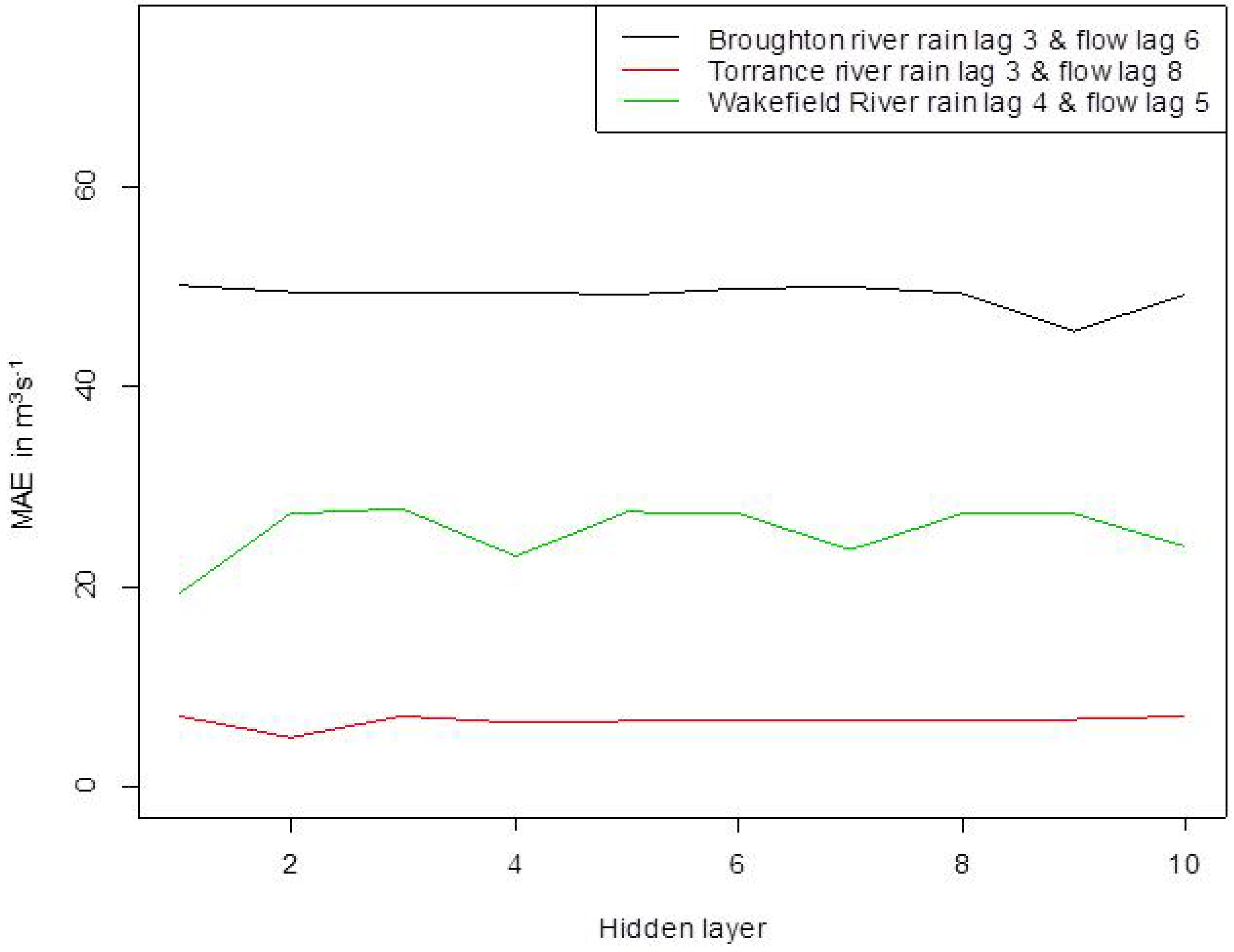
Application of back propagation in ANN with a sigmoidal function was used to set the normalized data in the MLP function. Furthermore, the mean absolute error (MAE) in m3s−1 was minimized through an iteration process that varied the number of nodes in the hidden layer.
The best lag combination at each location is presented in
Figure 6.
Figure 6.
MAE for training data (1990–2009) using ANN with best lag combinations at each location, units in m3s−1.
Figure 6.
MAE for training data (1990–2009) using ANN with best lag combinations at each location, units in m3s−1.
We find that both input lags and nodes in the hidden layer are different for each location. The best model based on correlation coefficient
and the lowest root mean square error (RMSE) and mean absolute error (MAE) for each location is presented in
Table 7. For Broughton River, 3 days rainfall and 6 days stream flow as lagged inputs with 9 nodes in the hidden layers produces the lowest MSE. At Torrance River, 3 days rainfall and 8 days stream flow as lagged inputs with 2 nodes in the hidden layers produces the lowest MSE. For Wakefield River, 4 days rainfall and 5 days stream flow as lagged inputs with only one node in the hidden layer produces the lowest MSE. This indicates the variability in the ANN models for different locations.
When the best model is identified based on the training data for each location, we use this model on testing data prediction. This study show the prediction results for the testing data for each location.
Figure 7 shows the predicted and observed stream flows using testing data for the locations Broughton River, Torrance River and Wakefield River, respectively.
Table 7.
Best prediction model based on , lowest RMSE and MAE are in m3s−1 on the training data.
Table 7.
Best prediction model based on , lowest RMSE and MAE are in m3s−1 on the training data.
| Location | Input Lags | Nodes in Hidden Layer in ANN(H) | | RMSE * | MAE * |
|---|
| Broughton River | 3 days rain, 6 days stream flow | 9 | 0.68 | 270.33 | 45.53 |
| Torrance River | 3 days rain, 8 days stream flow | 2 | 0.71 | 24.54 | 4.89 |
| Wakefield River | 4 days rain, 5 days stream flow | 1 | 0.45 | 179.42 | 19.28 |
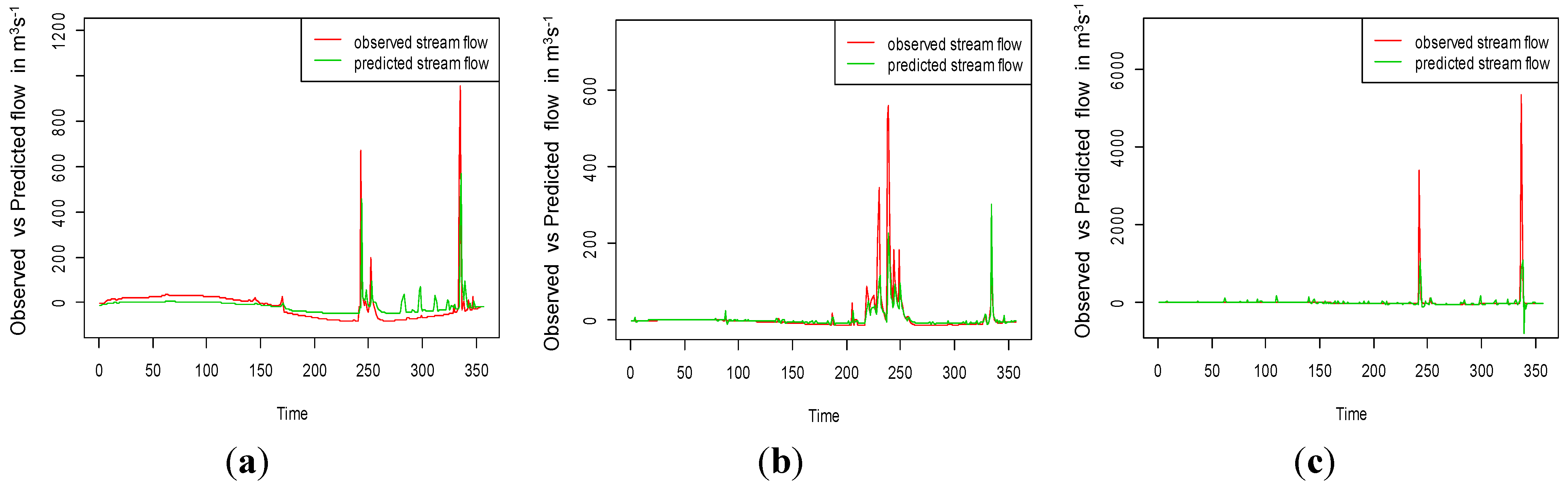
Figure 7.
Observed and predicted stream flow for (a) Broughton River; (b) Torrance River; and (c) Wakefield River for the year 2010.
Figure 7.
Observed and predicted stream flow for (a) Broughton River; (b) Torrance River; and (c) Wakefield River for the year 2010.
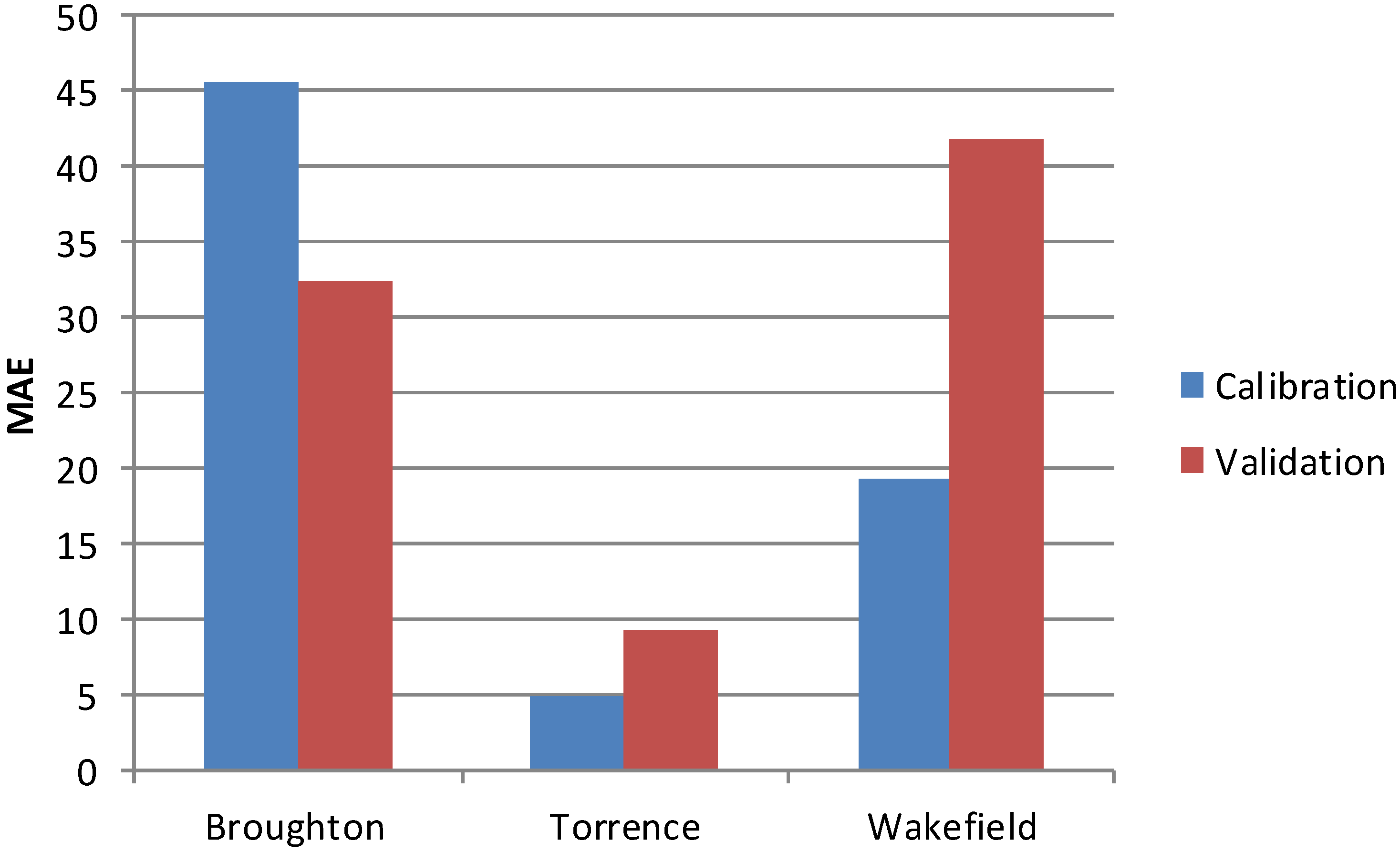
The MAE for training and testing data is shown in
Figure 8 for all three locations. We observed that the MAE for the training and testing data at Broughton and Torrance Rivers do not vary significantly.
For Broughton, in training, the best ANN model structure includes 3 days lagged rainfall and 6 days lagged stream flow as inputs with 9 nodes in the hidden layer. This model has the lowest MAE, at 45.53 m3s−1. We further use this best model for testing and we find the MAE of 32.43 m3s−1. For Torrance, the ANN best model in training has 3 days lagged rainfall and 8 days lagged stream flow as inputs with 2 nodes in the hidden layer achieving the MAE of 4.89 m3s−1. For testing data, this model gives a MAE of 9.27 m3s−1. In case of Wakefield, the best ANN model has 4 days lagged rainfall and 5 days lagged stream flow as inputs with 1 node in the hidden layer achieving the MAE of 19.28 m3s−1. For the testing data, this model achieves an MAE of 42.88 m3s−1. The reason for the difference in MAE between the training and testing phases could be due to this river’s ephemeral nature, and its substantial dependence on rainfall.
Figure 8.
Comparison of MAE for training and testing data, units are in m3s−1.
Figure 8.
Comparison of MAE for training and testing data, units are in m3s−1.


