Article

Hydraulic Features of Flow through Emergent Bending Aquatic Vegetation in the Riparian Zone

1
College of Water Conservancy and Hydropower, Hohai University, 1 Xikang Road, Nanjing 210098, Jiangsu, China
2
Sciences and Technology, University of Mascara, Mascara 29000, Algeria
*
Author to whom correspondence should be addressed.
Water 2013, 5(4), 2080-2093; https://doi.org/10.3390/w5042080
Submission received: 29 September 2013 / Revised: 27 November 2013 / Accepted: 5 December 2013 / Published: 13 December 2013
(This article belongs to the Special Issue Flood Estimation and Analysis in a Variable and Changing Environment)

Abstract

:
Vegetation in riparian zones has a significant influence on resistance, velocity distribution and turbulence intensity. This study experimentally investigated the effect of emergent bending riparian zone vegetation on the flow. The results showed that the frond and stem parts of Acorus calami had different influences on hydraulic features and that the relative depth ratio of water depth h to stem height hs was a key determinant of those influences. Manning coefficient n varied greatly with the variation of vegetation densities, relative depth ratio of water depth h to stem height hs, Re and Fr. Manning coefficient n increased with increasing vegetation density, particularly in cases when h/hs > 1. The velocity distributions did not follow logarithmic profiles, but they instead exhibited double logarithmic profiles. In addition, vegetation characteristics were shown to influence the height of maximum velocity. The position of maximum velocity is further away from the bed in cases with denser vegetation distribution. Finally, turbulence intensity showed more significant variation in the stem part and peaked near the middle of the stem, at z/hs = 0.5, where z was the distance from the bottom.

1. Introduction

A riparian zone has a complex ecotone; it is a transitional semiterrestrial area regularly influenced by fresh water that usually extends from the edges of water bodies to the edges of upland communities [1]. Riparian vegetation is a main focus of river restoration schemes, and the importance of its preservation to river ecology has also been noted [2]. Riparian vegetation has many ecological, aesthetic and economic benefits, such as providing terrestrial wildlife habitat; improving water quality; stabilizing streambanks and floodplains; supplying energy subsidies for aquatic and terrestrial ecosystems [3]; and serving as an important buffer in a healthy river ecosystem. Riparian zone revegetation has also been identified in recent years as one of the most common river restoration practices to obtain a more natural state [4,5]. For instance, Acorus calamus, which flourishes in riparian zones, has been extensively used in river restoration projects in China. Vegetation preservation is significant in the ecology of natural and artificial systems [6]. However, from an engineering point of view, riparian vegetation practices have not been often encouraged because of increased flow resistance, sediment transport effects and decreased flood discharge efficiency compared to unvegetated regions [7]. Thus, a better understanding of the physical processes governing flow resistances in vegetated areas could help resolve these conflicting engineering and ecological considerations [8].
With growing interest in river restoration and flood management requirements, several studies on the hydraulic properties of riverine vegetation have been conducted. Stephan and Gutknecht (2002) reported that Gessner who emphasized the importance of the alteration of flow velocity due to macrophyte communities was one of the first biologists [9]. Since then, many laboratory, numerical, analytical and field studies have been conducted to account for the complex dynamic interactions between vegetation and moving fluids [5,10]. For example, Kouwen et al. [11,12] studied the interaction between flexible vegetation and flow and reported that vegetation increases flow resistance, changes backwater profiles, and modifies sediment transport and deposition [11,12]. López and García (2001) proposed a κ-ε model to compute the mean velocity profile and turbulence characteristics in open channel vegetated flows [6]. Defina and Bixio [13] explored the capability of two different mathematical models to predict fully developed one-dimensional open channel flow in the presence of rigid, complex-shaped vegetation with submerged or emergent leaves.
Many previous studies concentrated on determining roughness coefficients to develop design methods [2]. In terms of submerged degree, aquatic plants in riparian zones fall into two categories: submerged plants and non-submerged (emergent) plants. Accordingly, flow resistance problems are usually classified into two groups: flow over submerged, short vegetation and flow through non-submerged (emergent), tall vegetation [14]. Most efforts to study vegetal resistance have concentrated on submerged plants and rigid roughness [14]. For simplification, plants have been simulated by a group of cylinders of the same height and diameter with regular spacing. Stone [15] conducted laboratory experiments to explore the hydraulic flow in an open channel with cylindrical roughness. Wilson, et al. [2] performed laboratory experiments on the effects of two forms (rods or stipes) of submerged flexible vegetation on the turbulence structure within the canopy and above the canopy region based on stiffness calculations. These studies would seem to characterize the flow regardless of the vegetation’s rigidity [16,17]. However, in terms of stiffness, aquatic plants are commonly classified into three groups: flexible, rigid and semi-flexible. Flexible and rigid plants have been more extensively studied, while few investigations have explored the mechanical response of semi-flexible plants. To address the new objectives of river restoration and environmental flood management, a better understanding of hydraulic flow features through emergent semi-flexible aquatic plants in riparian zones is required.
In this study, we focus on hydraulic flow features through Acorus calami, a typical emergent semi-flexible macrophyte, which can be divided into frond and stem. For simplification, an artificial A. calamus is used to conduct the experiments in a flume. The frond and stem have different influences on drag force, mean velocity profile and turbulence structure. The primary objective is to investigate the features of Manning coefficient n, mean velocity profiles and turbulence structures in the frond and stem of the emergent bending macrophytes.

2. Laboratory Experiments
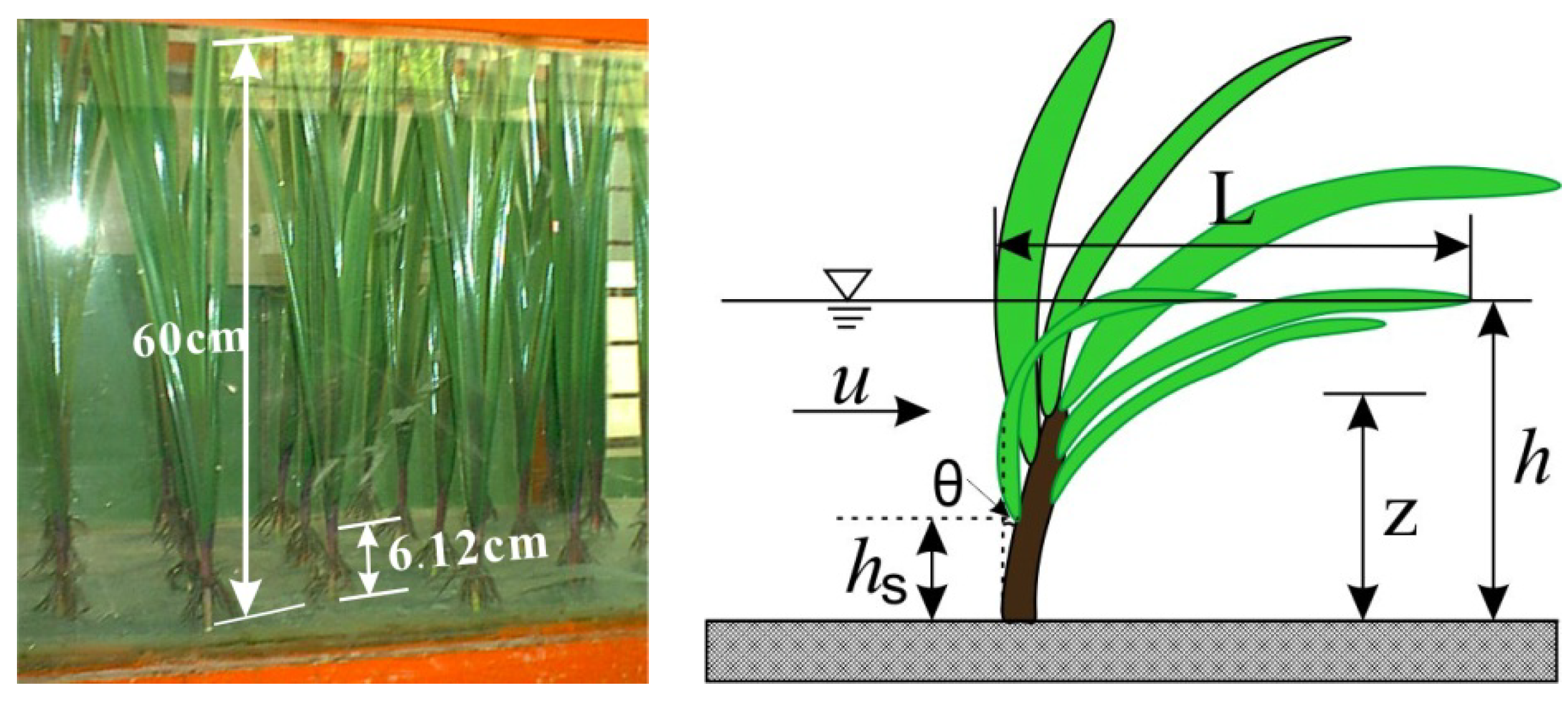
2.1. Materials

Acorus calamus is a tall perennial monocot of the Acoraceae family and is prevalent in riparian zones and in sunny locations. Mature Acorus calami are, on average, 50–120 cm high. Its leaves are sword shaped and are from 55 to 80 cm long and between 0.7 and 1.7 cm wide. In natural riparian zones, emergent vegetations exhibit three different primary motions under the impact of flow: erecting, compressing and bending [18]. A. calami stand rigid in water with a low flow velocity. As the discharge or water depth increases, the drag force on the plants increases as well, so the stems cannot withstand the flow and start to bend. This serves as a self-protection reaction, in that the vegetal element decreases its frontal area to decrease the drag force [18,19]. Individual natural A. calami have particular properties (e.g., height, stiffness), which hinder the generalization of the hydraulic features of natural A. calami. To investigate the hydraulic flow features of A. calami, it is necessary to use plant forms that are simplified and generalized compared to the complexity of real vegetation assemblages [2]. This is a similar approach to that adopted by other authors (e.g., Nepf and Vivoni 1999; Wilson, et al. 2003) [2,17]. In the present study, artificial plants manufactured from PE plastic were used to simulate natural A. calami. All parameters, including geometric, physical and kinematic parameters, were scaled using Froude’s law. In general, the dimensional parameters are 1:1 scale replicas of A. calami. The simulated A. calami are from 0.55 m to 0.7 m high and have 6 leaves from approximately 0.005 m to 0.018 m wide and between 0.65 m and 0.75 m long. They have basal stems with a mean diameter of 0.0115 m and mean height of 0.0612 m. The geometry and notation of simulated A. calami are shown in Figure 1. In addition, the bending stiffness (defined as the gradient of the force-deflection curves) of real and simulated A. calami are evaluated in the laboratory using the approach of Wilson (2003) [2]. The bending stiffnesses of natural and manufactured A. calamus are 14.35 N/m and 13.42 N/m, respectively. All geometric and physical parameters of natural and manufactured A. calami satisfy the Froude similarity rule.
Figure 1. Geometry and notation of simulated A. calami in flow.
Water 05 02080 g001

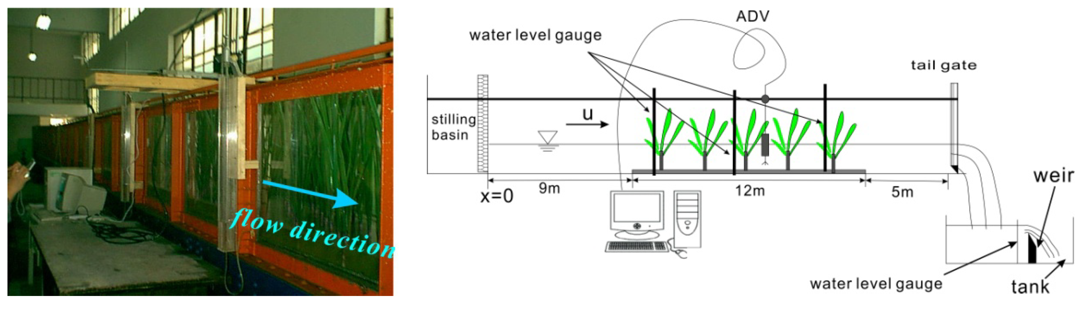
2.2. Experimental Setup and Measurement Technique

The experiments were conducted in a 26-m-long, 0.5-m-wide and 0.7-m-deep glass-walled flume (Figure 2). The slope of the flume is fixed at 0.07692%. Water was pumped into a stilling basin and flowed into the flume. The test region (12 m in length) is located 9 m from the entrance section. Upstream and downstream of the test segment, there were two transition segments (12 m and 5 m in length, respectively). The water surface profiles were controlled by the downstream tailgate, which was installed at the end of flume and could be adjusted using a gear system that allowed the opening size to be prescribed with a high degree of accuracy. The two transition segments and the tailgate prevented large-scale disturbances from the inlet and outlet and allowed for the development of a quasi-constant water flow by depth. The outlet and inlet of the flume were both connected to a tank, which enables the continuous recirculation of steady discharges.
Figure 2. Schematic of experimental setup.
Water 05 02080 g002
To ensure uniform conditions, the flow depths were controlled and measured using three water level gauges at three cross sections along the flume (10 m, 15 m, and 20 m from the entrance section), and the tailgate was adjusted as needed. Discharge was measured using the overflow weir and a water level gauge in the water-receiving channel. 3D mean velocities and velocity fluctuations were measured using a 3D sideways-looking Acoustic Doppler Velocimeter (ADV) manufactured by SonTek Inc., (San Diego, CA, USA). The ADV was mounted in a wood frame across the center section of the test segment, and it could be easily moved upstream or downstream, so that all sampling points were vertically aligned. The ADV technology is based on the pulse-to-pulse coherent measuring method. The instrument consists of three modules: a measuring probe, a conditioning module, and a processing module [20]. Mean velocities and velocity fluctuations can be measured from a small sampling volume (approximately 0.125 cm3), which is 5 cm away from the sensing elements. The probe was connected to the computer via a processing card. Real-time data could be recorded using a data acquisition program installed in the sampling computer. For each measurement, the sample-reporting rate was 25 Hz, and the acoustic frequency was 10 MHz. The velocity components, u, v, and w, correspond to the stream-wise (x), lateral (y), and vertical (z) directions, respectively. A 180-second sampling period was set for each test run. The WinADV-program, a post-processing program, was used to filter and post-process the sampled data. Data with average correlations less than or equal to 70% were filtered out.

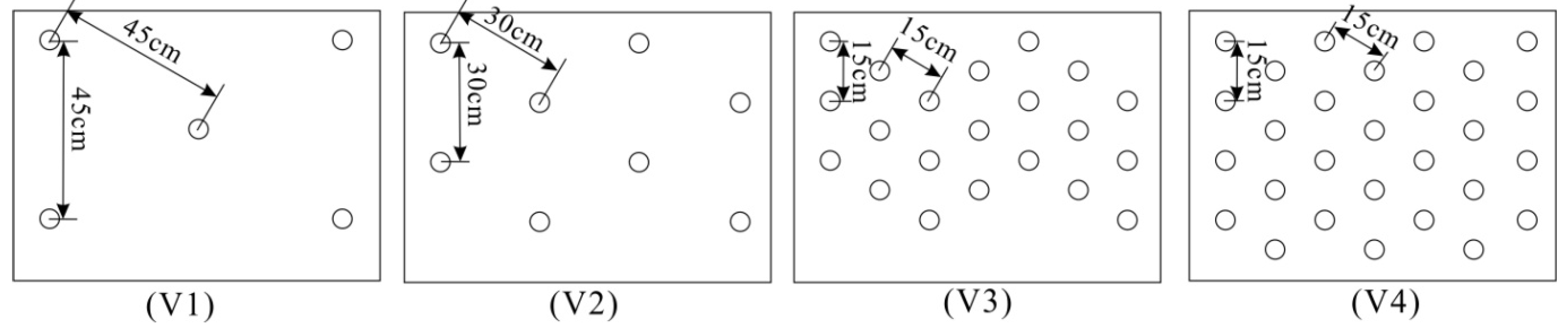
2.3. Test Series Description

Plants were placed into a PVC board platform with dimensions of 12 m × 0.5 m × 0.02 m (length, width and thickness in the principal flow direction, respectively) with prepared holes. The platform was fitted onto the bed of the test segment, 9 m away from the flume entrance segment (shown in Figure 2). The plants were arranged in a staggered pattern, with spacing of 15 cm, 30 cm and 45 cm, by sticking the end of the plant into the drilled holes. The arrays of plant arrangements are shown as V1, V2, V3 and V4 in Figure 3. V1 represents one or two plants in a row, with a spacing of 45 cm and a total of 40 plants in the test region. V2 shows two plants in a row, with a spacing of 30 cm and a total of 60 plants in the test region. V3 indicates three plants in a row, with a spacing of 15 cm and a total of 240 plants in the test region. V4 shows four plants in a row, with a spacing of 15 cm and a total of 280 plants in the test region. In addition, we explored the flow features of a non-vegetation flume, which is symbolized by V0.
Figure 3. Vegetation distribution patterns.
Water 05 02080 g003
Depending on the vegetation set-up, 8–9 h-Q combinations have been tested for each vegetation distribution pattern to investigate the influence of the ratio of water depth h on the stem height hs and h/hs, as well as the influence of the vegetation density, δ, on Manning coefficient n and the velocity distribution. Data for the 5 test series, with a total of 44 test runs, have been obtained in this study. A summary of the test series is presented in Table 1. In all the test series, the Reynolds numbers, Re, ranged from approximately 5600–48,000, indicating that all of the test runs are within the range of turbulent flow. The Froude numbers, Fr, ranged from 0.070 to 0.604, which means that all test runs can be considered subcritical flow. The plants exhibited no bending but instead oscillated slightly with low discharge. Conversely, because the leaves are flexible, the stems bend somewhat, and the leaves are streamlined with higher discharge. Furthermore, for each vegetation distribution pattern, the greatest discharge run (circled data in Table 1) has been selected to investigate flow velocity distribution and turbulence by water depth.
Table 1. Summary of experiments for vegetation density series.
SeriesDescriptionTest runsQ(m3/s)ReFrh(cm)u(m/s)
V0No vegetationV0-10.00650129960.5024.090.318
V0-20.00796159180.5274.530.351
V0-30.01090217920.5335.550.393
V0-40.01347269420.5326.400.421
V0-50.01900380000.5148.230.462
V0-60.02140427810.5108.950.478
V0-70.02520503940.5669.320.541
V0-80.03095618010.60410.220.605
V145 cm, 40 plantsV1-10.00616123240.2676.010.205
V1-20.00804160720.2786.980.230
V1-30.01040208050.2698.470.246
V1-40.01208241590.2639.510.254
V1-50.01514302730.24811.500.263
V1-60.01612322460.23812.340.261
V1-70.01879375710.22414.200.265
V1-80.02204440800.22115.950.276
V1-90.02391479220.21617.100.280
V230 cm, 60 plantsV2-10.0049899570.2265.820.171
V2-20.00606121270.2336.510.186
V2-30.00843168610.2278.250.205
V2-40.00902180440.2248.720.207
V2-50.01154230740.21710.490.220
V2-60.01381276100.21411.930.231
V2-70.01405281030.20712.350.228
V2-80.01854370770.18815.850.234
V2-90.02056411210.17018.130.227
V315 cm, 240 plantsV3-10.0028893200.1305.750.100
V3-20.0036973720.1187.360.100
V3-30.0046657520.1338.060.116
V3-40.00530106000.1219.230.115
V3-50.00610121950.12210.050.121
V3-60.00750149990.10712.560.119
V3-70.00980196020.09016.730.117
V3-80.01158231520.08120.260.114
V3-90.01290257580.07022.800.113
V415 cm, 280 plantsV4-10.0029859550.1046.940.086
V4-20.0030561000.1047.050.087
V4-30.0035069990.1087.550.093
V4-40.0042083970.1188.010.105
V4-50.00550109960.1219.450.116
V4-60.00618123570.11410.630.116
V4-70.00640127850.10911.220.114
V4-80.00736147140.09813.220.111
V4-90.01090218010.07919.860.101

3. Analytical Method

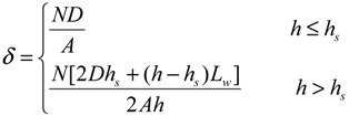
3.1. Vegetation Density

Most previous experiments have been conducted with arrays of rigid emergent cylindrical elements of constant diameter, where the momentum absorbing areas of the plant were constant with plant height. In these cases, the density was defined as the projected area of rod per volume [2,19]. This definition can be extended to quantify the vegetation density for emergent semi-flexible plants. Vegetation density can be defined as the momentum absorbing area per unit water volume. Determining the momentum absorbing area is a topic of significant concern. In some previous studies, the total momentum absorbing area is represented by the total frontal area of plants [21,22]. However, because wetted leaves spread in the flow direction in water, considerable foliage area is hidden behind the frontal area. Thus, it is important to use the total wetted surface area instead of the total frontal area in these calculations. In practice, the wetted surface area consists of the wetted stem surface area and the wetted frond surface area. When the water depth is deeper than the stem height, both the wetted stem surface area and the wetted frond surface area should be considered. Otherwise, only the stem area should be considered. Vegetation density can be described as in Equation (1):
Water 05 02080 i001
where δ is the vegetation density, m−1; N is the total number of plants; D is the diameter of stem, m; A is the area of testing reach, m2; h is the water depth, m; hs is the height of stem, m; and Lw is the width of wetted foliage, m.
In Equation (1), all parameters (aside from Lw) can be easily obtained. However, because Lw mainly depends on the bending degree, it cannot be directly determined. In this study, Lw is determined statistically using the geometric mean after measuring the wetted foliage widths of 20 plants for each test run.

3.2. Resistance Coefficient

Estimating the flow resistance of vegetation is of great importance in river management because of its potentially significant effects on channel conveyance [14]. Efforts to quantify hydraulic roughness in vegetated channels date to the 1950s and 1960s [5]. The methods for quantifying resistance vary from one-dimensional approaches (e.g., Manning coefficient or Darcy-Weisbach friction factor) to three-dimensional approaches based on the drag force equation. Järvelä (2002) calculated the Darcy-Weisbach friction coefficient based on measured head losses [14]. In practice, Manning coefficient n is the most widely used resistance quantifying metric in river hydraulics. Many previous studies have presented Manning coefficient n as a function of hydraulic radius, vegetation density, vegetation stiffness, and plant frontal area. Flow resistance is dominated by vegetation resistance, and the vegetation drag coefficient is used as a fitting parameter [21]. In this study, Manning coefficient n is calculated using Equation (2) proposed by Fischenich (2000), which is based on the drag force concept [23].
Water 05 02080 i002
where R represents hydraulic radius; Cd is the effective vegetal drag coefficient; Aveg is the frontal area of the vegetation; and kn is the units term.

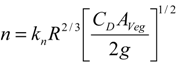
3.3. Turbulence Intensity

The quantitative analysis of turbulent flow is based on measurements of velocity fluctuations at a single point in the flow (or at multitude points, from which the flow fields can be inferred). In this study, the mean flow velocity components (u, v, and w) and velocity fluctuation components in turbulent flow (u', v', w') correspond to the streamwise, lateral and vertical directions, respectively. Velocity fluctuations can be defined as the deviation from the mean velocity. In general, root-mean-square values (RMS) of velocity fluctuations are considered measures of turbulence intensities. Turbulence intensities corresponding to streamwise, lateral and vertical directions are defined as follows [24]:
Water 05 02080 i003
where N is the total number of observations in a given series; u', v' and w' are velocity fluctuations of streamwise flow, lateral flow and vertical flow, respectively; and RMSu, RMSv and RMSw are turbulence intensities corresponding to streamwise, lateral and vertical flow, respectively.

4. Results and Discussion

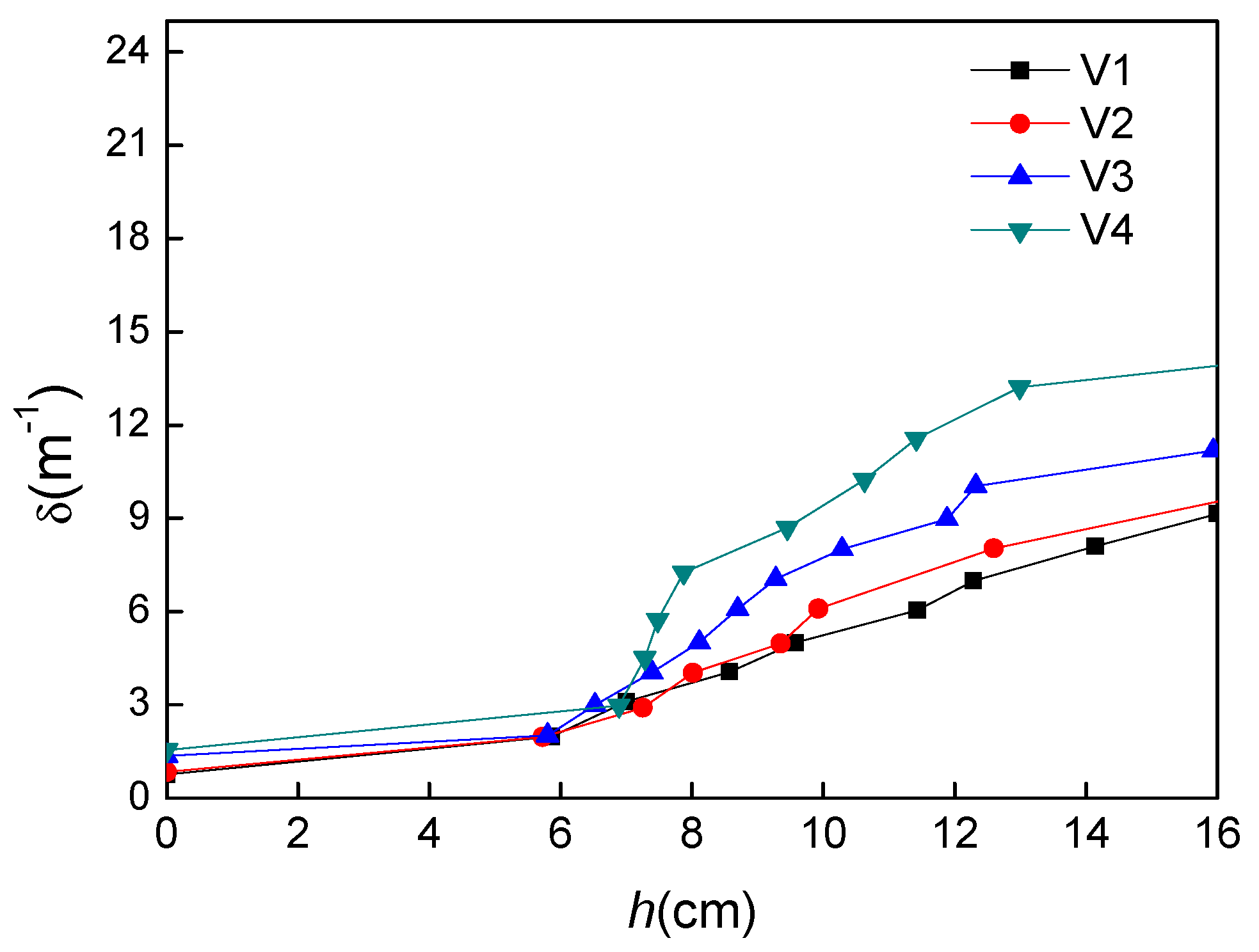
4.1. Vegetation Density

The profiles of vegetation densities δ against water depth h for the four vegetation distribution patterns are plotted in Figure 4. Figure 4 illustrates that vegetation density increases with rising water level in all cases. However, when the water level is lower than stem height, only minimal increases in vegetation densities can be observed. Conversely, much more significant increases in vegetation densities can be observed at greater h. Furthermore, the V4 cases show the largest increasing rate of vegetation density for h/hs > 1, while the V1 cases have the least increase rate of δ.

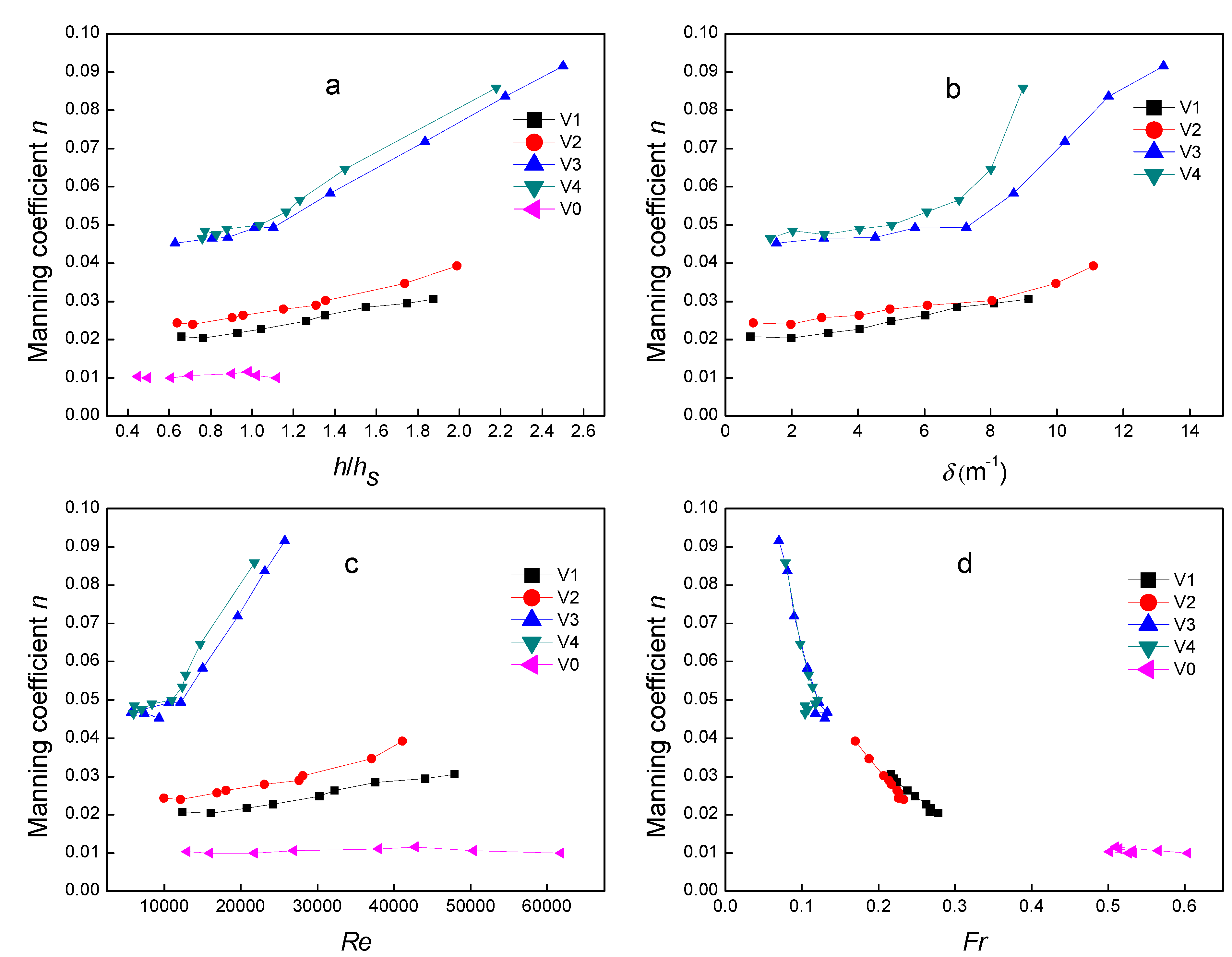
4.2. Manning Coefficient n

In this study, Manning coefficient n is used as a measure of flow resistance. The total resistance of the flume includes sidewall and vegetation bottom resistance, designated as nw and nb, respectively. Because the flume wall is glass, its resistance can be considered negligible compared to that of vegetation. In other words, the flow resistance in a vegetated flume is dominated by the vegetation bottom resistance. The flow resistance n = nb can be evaluated by applying Equation (2). After investigating various test runs, it may be concluded how Manning coefficient n varies with the relative depth ratio of water depth h to stem height hs, the vegetation density and the Reynolds number. These are shown in Figure 5a–d.
Figure 4. Profiles of vegetation densities against water depth in different vegetation distribution patterns, where h is the water depth and δ is the vegetation density.
Water 05 02080 g004
Figure 5. Manning coefficient n for each series: (a) n against relative depth ratio, h/hs, where h is the water depth and hs is the plant stem height; (b) n against vegetation density, δ(m−1); (c) n against Reynolds number, Re; (d) n against Froude number, Fr.
Water 05 02080 g005
Figure 5 shows that the Manning coefficient n of vegetation flow (e.g., V1, V2, V3 and V4) is greater than that of non-vegetation flow (e.g., V0). Additionally, Figure 5 illustrates that the Manning coefficient has great variation with the distance between two plants. When the distance between two plants is less under the same discharge situation, the Manning n becomes greater. The sequence is V4 > V3 > V2 > V1. It is similar to Hall’s results [25]. Furthermore, Figure 5a shows that the Manning coefficient n increases with increasing the ratio of water depth to plant stem height h/hs. However, the increment of change in n below the stem height (h/hs = 1.0) is less than that above the stem height. When the ratio of flow depth to plant stem height, h/hs < 1, the n increment is approximately 3%. Conversely, when h/hs > 1, the Manning n increments are approximately 5.7%, 7.7%, 16.4%, 23.2% at V1, V2, V3 and V4, respectively. It illustrates that the contribution of foliage with flexible leaves is significantly greater than that of plant stems without leaves. Thus, variations in Manning n depend on the position of the separating point between the stem and foliage. The leaf is found to be an important factor in the analyses, and properties such as rigidity are found to influence the drag exerted by leaves. This can also be illustrated by Figure 5b. When the vegetation density is less than approximately 6.5 m−1, an increasing trend of Manning n is not apparent. However, when the vegetation density is greater than 6.5 m−1, the Manning n increases more significantly with increasing vegetation density. Manning coefficient is almost uniform up to the critical plant density and then increases [6].
Figure 5c also shows that the general tendency is an increase in the n value with increasing Reynolds number Re. Additionally, in high dense distribution (V3 and V4), the increase tendency is very dramatical when Re > 10,000. It implies that Re = 10,000 would be a critical Renolds number. When the Re < 10,000, the flow would be laminar flow. Otherwise, it is transit flow or turbulent flow. Figure 5c shows that the Renolds number Re the distance between two plants Figure 5d indicates that the Manning n decreases with increasing Fr. Therefore, the separating point and water depth are the definitive factors which have most important influence on the Manning coefficient n.

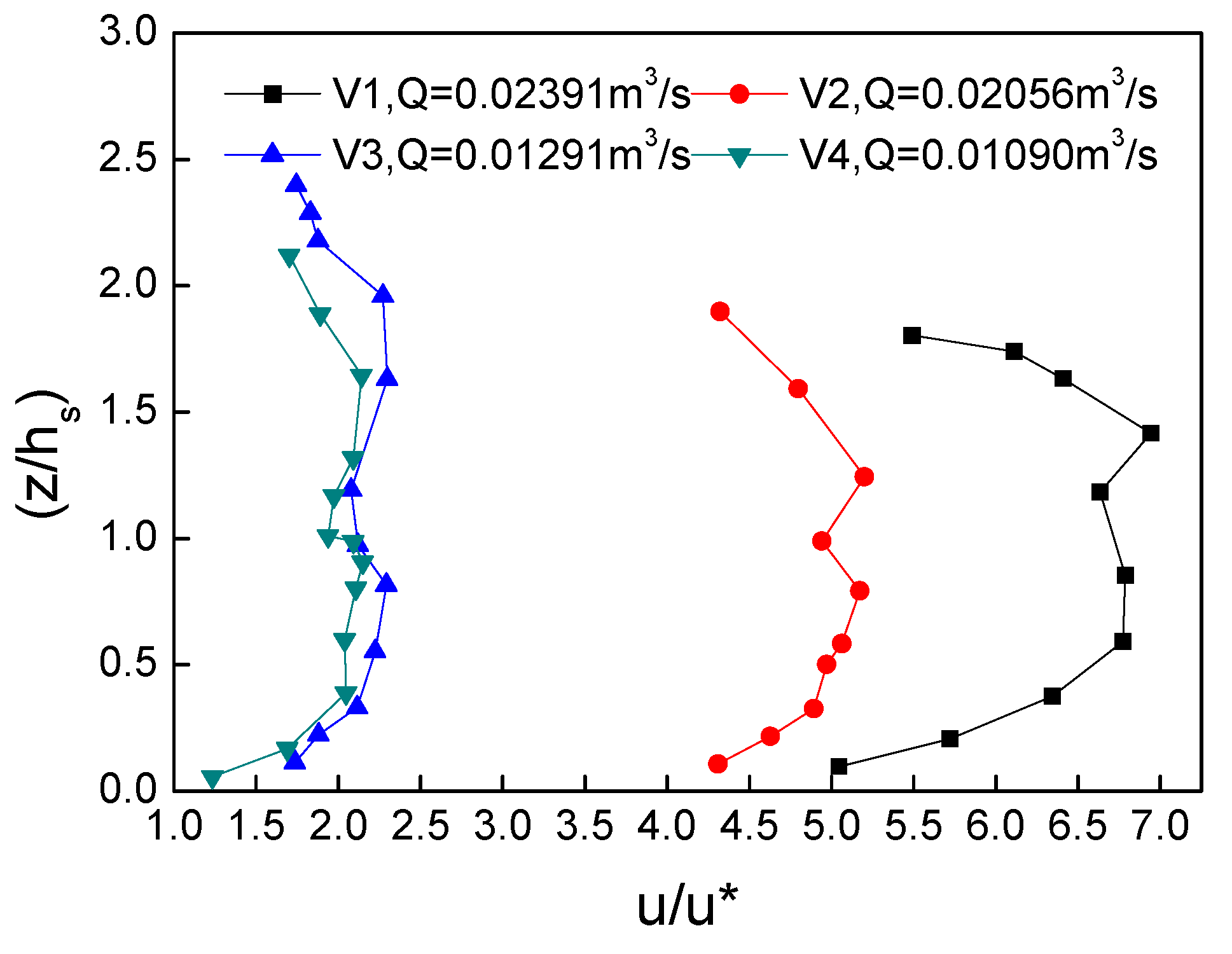
4.3. Velocity Distribution

Velocities at any point can be measured in three mutually perpendicular directions: streamwise (parallel to the boundary, u), lateral (normal to the boundary, v) and vertical (w). The test runs V1-9, V2-9, V3-9 and V4-9, which are the largest discharge runs for different vegetation density patterns (0.02391 m3/s for V1, 0.02056 m3/s for V2, 0.01290 m3/s for V3 and 0.01090 m3/s for V4), are used to investigate velocities and turbulence intensities in x, y and z directions. The sampling vertical line stands at the center of four neighboring plants. The surveyed velocity profiles are shown on the plane z/hs against u/u* (Figure 6), where z is the distance from the bed, hs is the plant stem height and u* is the shear velocity estimated using Water 05 02080 i004, where J is the flume slope [26].
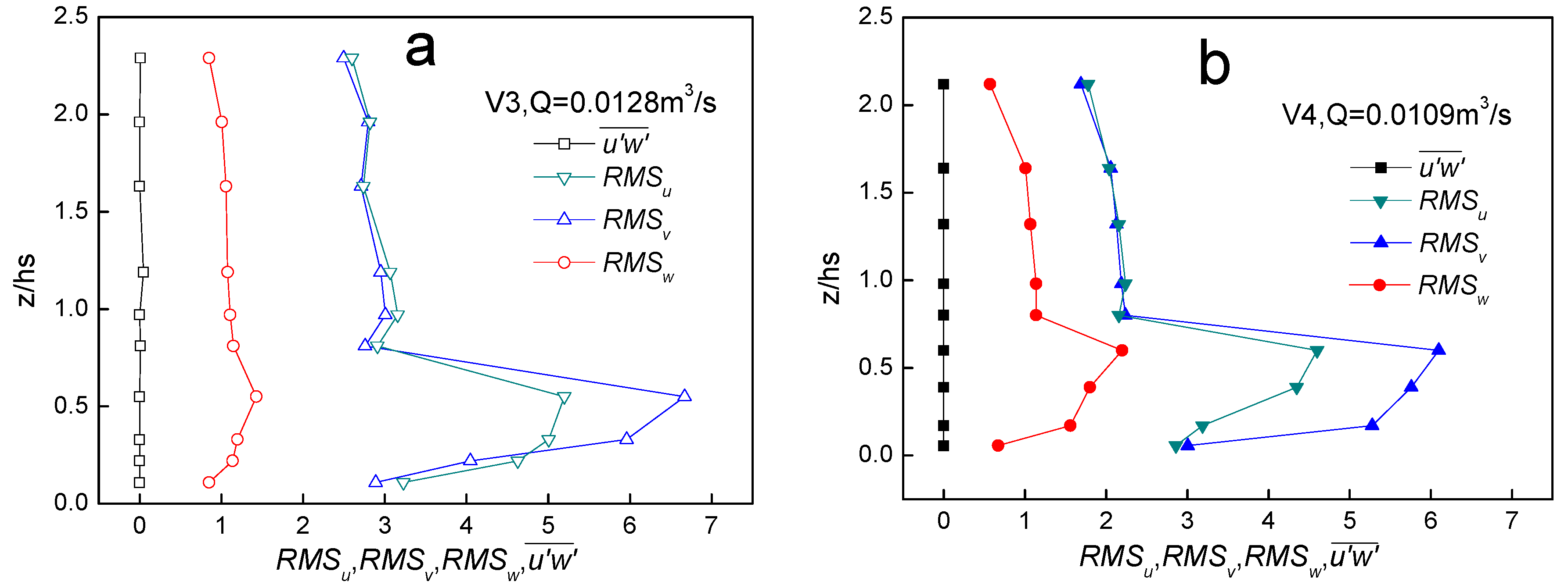
For all experimental test runs with Re > 12,500 and Fr < 1, vegetation flows are considered to be turbulent subcritical flows. Figure 6 shows that the mean flow with plants is greatly slowed and no longer follows a logarithmic vertical profile. From the velocity profiles, two zones can be distinguished: the stem part (z/hs < 1) and the foliage part (z/hs > 1). However, because both profiles in the stem and foliage parts almost follow logarithmic behavior, the whole velocity profile can be characterized as a double logarithmic profile. Furthermore, both the stem and foliage parts have significant variations in mean velocities and exhibit the generation of a horizontal shear layer. The magnitude of the mean velocity in the foliage part is less than that in the stem part because the foliage consumes much more energy and momentum from the flow through the generation of turbulence. A local velocity maximum can be observed near the bed in the stem part. In addition, Figure 6 shows that vegetation densities have some influence on the vertical velocity distribution. The vertical velocities of V3 and V4 are much lower than those of V1 and V2, as expected. Figure 6 also shows that the position of maximum velocity is farther from the bed in the denser vegetation distributions. This result is similar to the report by Afzalimehr, et al. [27].
Figure 6. Vertical velocity distribution profiles.
Water 05 02080 g006

4.4. Turbulence

In each vegetation distribution pattern, the largest discharge run was investigated to measure the turbulence intensities and Reynolds stress (u'w', instantaneous streamwise velocity fluctuations multiplied by the instantaneous vertical velocity fluctuations, then time averaged). For example, the turbulence intensities (RMSu, RMSv, RMSw) and Reynolds stress (u'w') for V3 (Q = 0.0129 m3/s) and V4 (Q = 0.0109 m3/s) are shown in Figure 7a,b, respectively.
Figure 7. Turbulence intensities and Reynolds stress against relative depth ratio of vertical distance from bed z to stem height hs: (a) represents V3 pattern and Q = 0.0128 m3/s; (b) represents V4 pattern and Q = 0.0109 m3/s.
Water 05 02080 g007
Figure 7a,b show that the Reynolds stress is quite small and can be considered zero (u'w' ≈ 0). This finding indicates that the turbulent transport of momentum in the vertical direction is so small that the Reynolds stress can be neglected.
Figure 7 also shows that the turbulence intensity distribution is anisotropic. In general, turbulence intensity in the z direction is much smaller than that in the other two directions. As z/hs > 1, turbulence intensity has little variation and can be considered constant. However, the turbulence intensity varies dramatically for 0 < z/hs < 1. The turbulence intensity peaks near the middle of the stem. In another words, turbulence intensity increases for z/hs < 0.5 and decreases for 0.5 < z/hs < 1. Afzalimhr, et al. [27] reported similar results of approximately constant turbulence intensity above the stem height. When the water depth is higher than the stem height, the flexible leaves bend over in the flow when the discharge is high. As the leaves become parallel to the flow, the momentum flux is absorbed, decreasing the turbulence intensity of the flow within the canopy. While the foliage induces a greater drag force, the turbulence generated by shear is reduced due to the inhibition of momentum exchange by the plant frontal area. In conclusion, the stem and foliage of emergent bending aquatic vegetation have quite different effects on the turbulence intensity of the flow, with more intense turbulence in the stem regime.

5. Conclusions

This paper presented an experimental study that explored the effect of emergent bending vegetations on the Manning coefficient n, the velocity distribution and turbulence structure within the stem and foliage for various distribution combinations. In this study, simulated A. calami, 1:1 scaled with a real plant, were arranged into four density patterns in a laboratory flume. An ADV was used to measure the mean velocities and velocity fluctuations.
Compared with non-vegetation flow, vegetation flow in riparian zones was characterized as having larger Manning coefficients n, a non-log law of mean velocity profiles and obvious turbulence. Furthermore, these features depended significantly on the vegetation properties, densities and distribution patterns. Particularly, because the frond and stem parts of A. calami had different influences on hydraulic features, the ratio of water depth to stem height h/hs was a key factor for investigating the hydraulic features of this species. For instance, Manning coefficient n varied greatly with the variation of vegetation densities δ, relative depth ratio h/hs, Re and Fr. Manning coefficient n increased with the increasing vegetation density and increased more rapidly in cases with h/hs > 1.
Vertical velocity profiles did not follow logarithmic profiles. According to the vertical velocity distribution, the flow could be separated into two zones: a stem zone and a foliage zone. In general, the velocity distribution showed double logarithmic profiles. The magnitude of the mean velocity in the foliage zone was less than that in the stem zone. Vegetation densities were shown to be influential on the vertical velocity distribution. The peak point of velocity was further away from the bed in cases with denser vegetation distributions. Therefore, vegetation played an important role in the boundary layer thickness and the height of maximum velocity.
For emergent vegetation, the Reynolds stresses within vegetations were quite small, and the turbulence intensities were found to be anisotropic. Turbulence intensities peaked at around z/hs = 0.5. This result indicates the presence of strong turbulence intensity around the stem and that bending flexible foliage weakened the turbulence intensities.
This work focuses on a single type of aquatic plant in riparian zone. However, riparian zones actually include erecting, bending and submerged plants. Further studies should investigate the interaction between flow and different vegetation types and combinations. Field surveys and additional laboratory experiments are planned.

Acknowledgments

This study was funded by the National Natural Science Foundation of China (NSFC) (Grant No. 40871050) and Water Resource Technology Foundation of Zhejiang Province, China (Grant No. RA1104). We are grateful to the Hydraulic Engineering Laboratory, Hohai University, for the use of laboratory facilities and to Zhongfu Fu, Mingming Liu and Jiacai Lu for their thoughtful comments on measurements during the laboratory research. Additionally, good suggestions and comments from Robert M. Holt (the University of Mississippi), Weiming Wu and Zhangping Wei (National Center for Computational Hydroscience and Engineering, the University of Mississippi) are greatly appreciated.

Conflicts of Interest

The authors declare no conflict of interest.

References

  1. Naiman, R.J.; Decamps, H.; McClain, M.E. Riparia: Ecology, Conservation, and Management of Streamside Communities; Elsevier Academic Press: New York, NY, USA, 2005; pp. 1–2. [Google Scholar]
  2. Wilson, C.A.M.E.; Stoesser, T.; Bates, P.D.; Pinzen, A.B. Open channel flow through different forms of submerged flexible vegetation. J. Hydraul. Eng. 2003, 129, 847–853. [Google Scholar] [CrossRef]
  3. Merritt, D.M.; Scott, M.L.; Poff, N.L.; Auble, G.T.; Lytle, D.A. Theory, methods and tools for determining environmental flows for riparian vegetation: Riparian vegetation-flow response guilds. Freshw. Biol. 2010, 55, 206–225. [Google Scholar] [CrossRef]
  4. Bernhardt, E.S.; Palmer, M.A. Restoring streams in an urban context. Freshw. Biol. 2007, 52, 738–751. [Google Scholar] [CrossRef]
  5. Stone, M.C.; Chen, L.; Mckay, S.K.; Goreham, J.; Acharya, K.; Fischenich, C.; Stone, A.B. Bending of submerged woody riparian vegetation as a function of hydraulic flow conditions. River Res. Appl. 2013, 29, 195–205. [Google Scholar] [CrossRef]
  6. López, F.; García, M. Mean flow and turbulence structure of open-channel flow through non-emergent vegetation. J. Hydraul. Eng. 2001, 127, 392–402. [Google Scholar] [CrossRef]
  7. Aberle, J.; Järvelä, J. Flow resistance of emergent rigid and flexible floodplain vegetation. J. Hydraul. Res. 2013, 51, 33–45. [Google Scholar] [CrossRef]
  8. Järvelä, J.; Aberle, J.; Dittrich, A.; Schnauder, I.; Rauch, H.P. Flow–Vegetation–Sediment Interaction: Research Challenges. In Proceedings of International Conference River Flow, London, UK, 6–8 September 2006; Ferreira, R.M.L., Alves, E.C.T.L., Leal, J.G.A.B., Cardoso, A.H., Eds.; Taylor & Francis: London, UK, 2006; Volume 2, pp. 2017–2026. [Google Scholar]
  9. Stephan, U.; Gutknecht, D. Hydraulic resistance of submerged flexible vegetation. J. Hydrol. 2002, 269, 27–43. [Google Scholar] [CrossRef]
  10. Chen, L.; Stone, M.C.; Acharya, K.; Steinhaus, K.A. Mechanical analysis for emergent vegetation in flowing fluids. J. Hydraul. Res. 2011, 49, 766–774. [Google Scholar] [CrossRef]
  11. Kouwen, N.; Li, R.M.; Simons, D.B. Flow resistance in vegetated waterways. Transp. ASAE 1981, 24, 684–698. [Google Scholar] [CrossRef]
  12. Kouwen, N. Modern approach to design of grassed channels. J. Irrig. Drain. Eng. 1992, 118, 773–743. [Google Scholar]
  13. Defina, A.; Bixio, A.C. Mean flow and turbulence in vegetated open channel flow. Water Resour. Res. 2005, 41, W07006. [Google Scholar]
  14. Järvelä, J. Flow resistance of flexible and stiff vegetation: A flume study with natural plants. J. Hydrol. 2002, 269, 44–54. [Google Scholar] [CrossRef]
  15. Stone, B.M.; Shen, H.T. Hydraulic resistance of flow in channels with cylindrical roughness. J. Hydraul. Eng. 2002, 128, 500–506. [Google Scholar] [CrossRef]
  16. Tsujimoto, T.; Shimizu, Y.; Kitamura, T.; Okada, T. Turbulent open-channel flow over bed covered by rigid vegetation. J. Hydrosci. Hydraul. Eng. 1992, 10, 13–25. [Google Scholar]
  17. Nepf, H.; Vivoni, E.R. Turbulence Structure in Depth-Limited Vegetated Flow: Transistion between Emergent and Submerged Regimes. In Proceedings of 28th International Association for Hydraulic Resources Congress, Graz, Austria, 22–27 August 1999.
  18. Yagci, O.; Tschiesche, U.; Kabdasli, M.S. The role of different forms of natural riparian vegetation on turbulence and kinetic energy characteristics. Adv. Water Resour. 2010, 33, 601–614. [Google Scholar] [CrossRef]
  19. Nepf, H.M. Drag, turbulence, and diffusion in flow through emergent vegetation. Water Resour. Res. 1999, 35, 479–489. [Google Scholar] [CrossRef]
  20. Carollo, F.G.; Ferro, V.; Termini, D. Flow velocity measurements in vegetated channels. J. Hydraul. Eng. 2002, 128, 664–673. [Google Scholar] [CrossRef]
  21. Kothyari, U.; Hayashi, K.; Hashimoto, H. Drag coefficient of unsubmerged rigid vegetation stems in open channel flows. J. Hydraul. Res. 2009, 47, 691–699. [Google Scholar] [CrossRef]
  22. Chen, S.; Kuo, Y.; Li, Y. Flow characteristics within different configurations of submerged flexible vegetation. J. Hydrol. 2011, 398, 124–134. [Google Scholar] [CrossRef]
  23. Fischnich, J.C. Resistance Due to Vegetation; Engineer Research and Development Center: Vicksburg, MS, USA, 2000. [Google Scholar]
  24. Robert, A. River Process: An Introduction to Fluvial Dynamics; Arnold, Distributed in the United States of America by Oxford University Press Inc.: New York, NY, USA, 2003; pp. 35–50. [Google Scholar]
  25. Hall, B.R.; Freeman, G.E. Study of hydraulic roughness in wetland vegetation takes new look at Manning’s n. Wetl. Res. Program Bull. US Army Corps Eng. Waterways Exp. Stn. 1994, 4, 1–4. [Google Scholar]
  26. Kironoto, B.; Graf, W.H. Turbulence characteristics in rough uniform open-channel. Proc. Inst. Civ. Eng. Waters Marit. Energy 1995, 106, 233–241. [Google Scholar]
  27. Afzalimehr, H.; Najfabadi, E.F.; Singh, V.P. Effect of vegetation on banks on distributions of velocity and Reynolds stress under accelerating flow. J. Hydrol. Eng. 2010, 15, 708–713. [Google Scholar] [CrossRef]

