Uncertainties in Flow-Duration-Frequency Relationships of High and Low Flow Extremes in Lake Victoria Basin


Abstract
:1. Introduction
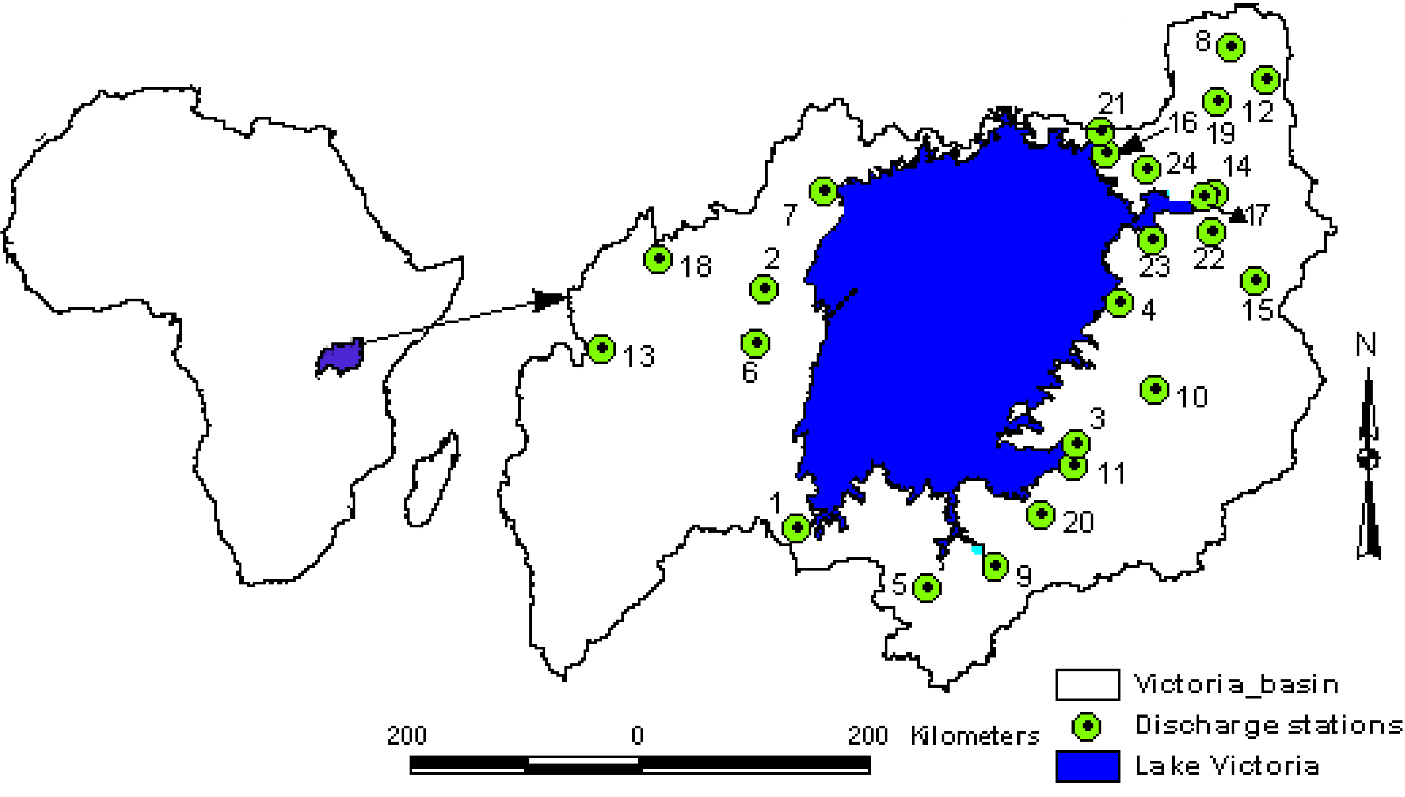
2. Study Area and Data Series


| Station number | River catchment | Station ID | Area [km2] | Data length [Year] | Location | Missing records [%] | ||
|---|---|---|---|---|---|---|---|---|
| From | To | Longitude [°] | Latitude [°] | |||||
| (1) | Biharamulo | *** | 1,981 | 1950 | 2004 | 31.29 | 2.62 | 13 |
| (2) | Bukora | 81270 | 8,392 | 1951 | 1976 | 31.48 | −0.85 | 16 |
| (3) | Grumeti | 5F3 | 13,363 | 1950 | 2004 | 33.94 | −2.06 | 19 |
| (4) | Gurcha-migori | 1KB05 | 6,600 | 1950 | 2004 | 34.20 | −0.95 | 3 |
| (5) | Isanga | 114012 | 6,812 | 1976 | 2004 | 32.77 | −3.21 | 12 |
| (6) | Kagera | 58370 | 54,260 | 1950 | 1994 | 31.43 | −1.29 | 20 |
| (7) | Katonga | 100006 | 15,244 | 1950 | 1975 | 31.95 | −0.09 | 18 |
| (8) | Koitobos | 1BE06 | 813 | 1949 | 1975 | 35.09 | 0.97 | 3 |
| (9) | Magogo-maome | 113012 | 5,207 | 1950 | 2004 | 33.15 | −2.92 | 19 |
| (10) | Mara | 107072 | 13,393 | 1950 | 2003 | 34.56 | −1.65 | 11 |
| (11) | Mbalangeti | 111012 | 3,591 | 1950 | 2004 | 33.86 | −2.22 | 14 |
| (12) | Moiben | 1BA01 | 188 | 1953 | 1990 | 35.44 | 0.80 | 16 |
| (13) | Nyakizumba | 100005 | 359 | 1950 | 1987 | 30.08 | −1.32 | 15 |
| (14) | Nyando | 1GD01 | 3,652 | 1962 | 2001 | 35.04 | −0.10 | 2 |
| (15) | Nyangores | 1LA03 | 4,683 | 1963 | 1993 | 35.35 | −0.79 | 10 |
| (16) | Nzoia | 1EF01 | 12,676 | 1974 | 1999 | 34.08 | 0.13 | 8 |
| (17) | Ogilla | 1GD03 | 2,650 | 1970 | 1996 | 34.96 | −0.13 | 1 |
| (18) | Ruizi | 100004 | 2,070 | 1970 | 1998 | 30.65 | −0.62 | 8 |
| (19) | Sergoit | 1CA02 | 659 | 1959 | 1990 | 35.06 | 0.63 | 2 |
| (20) | Simiyu Ndagalu | 5D1 | 1,205 | 1970 | 1996 | 33.56 | −2.63 | 12 |
| (21) | Sio | 1AH01 | 1,450 | 1958 | 2000 | 34.15 | 0.38 | 6 |
| (22) | Sondu | 1JG01 | 3,508 | 1950 | 1990 | 35.01 | −0.39 | 12 |
| (23) | South Awach | 1HE01 | 3,156 | 1950 | 2004 | 34.54 | −0.47 | 7 |
| (24) | Yala | 1FG01 | 3,351 | 1950 | 2000 | 34.51 | 0.09 | 3 |
3. Methodology
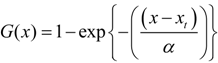
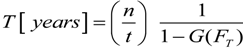
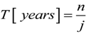
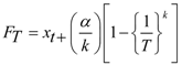
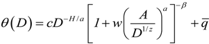
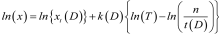
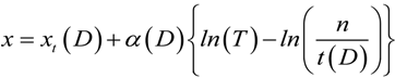
3.1. FDF Modeling
 , for k = 0
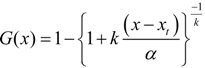 , for k ≠ 0
 , for k ≠ 0
 , for k = 0

 , for k ≠ 0
 , for k = 0
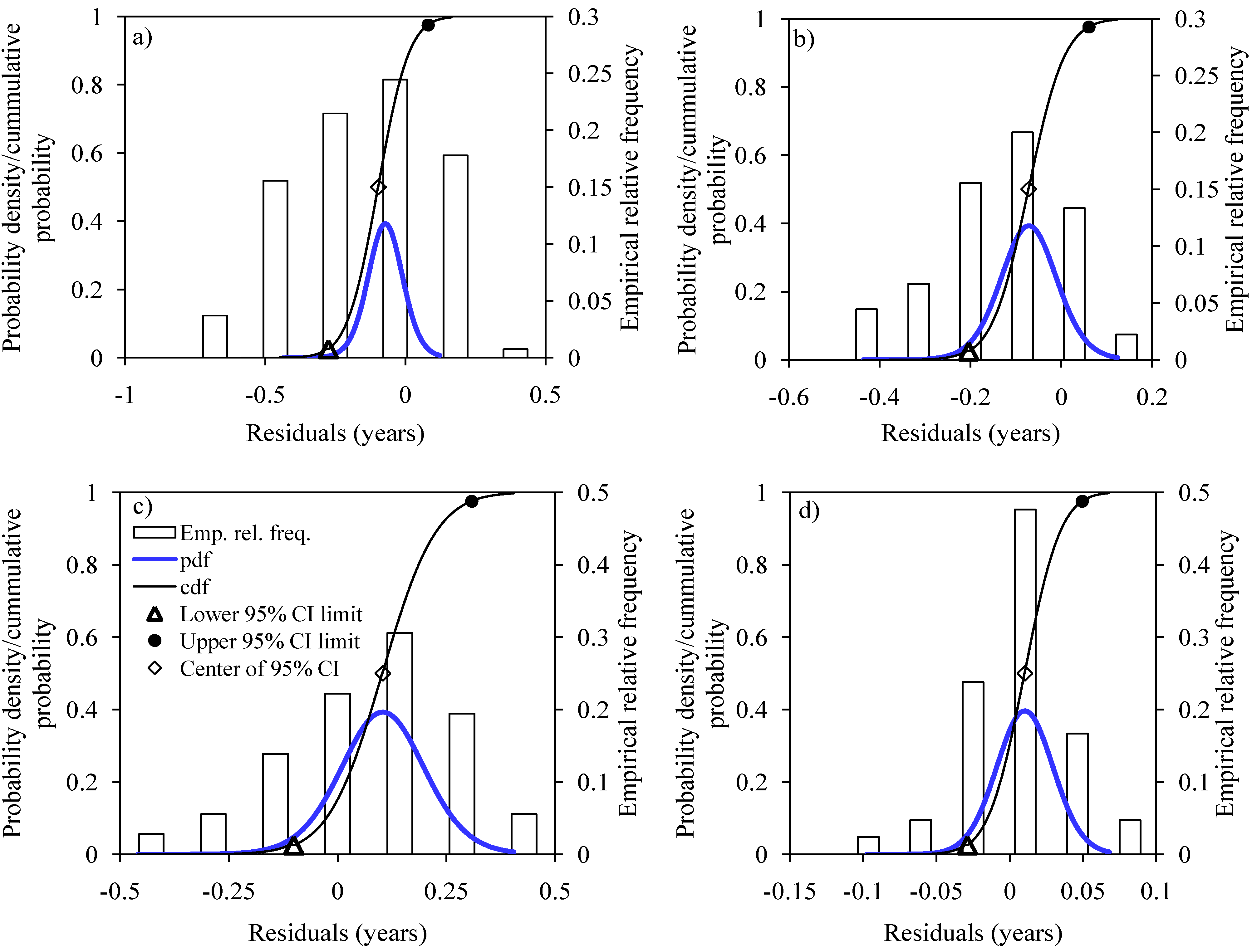
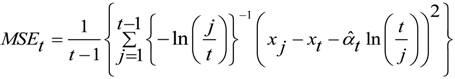
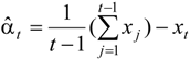
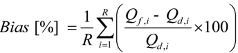
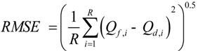
3.2. Uncertainty and Error Analysis
4. Results and Discussion
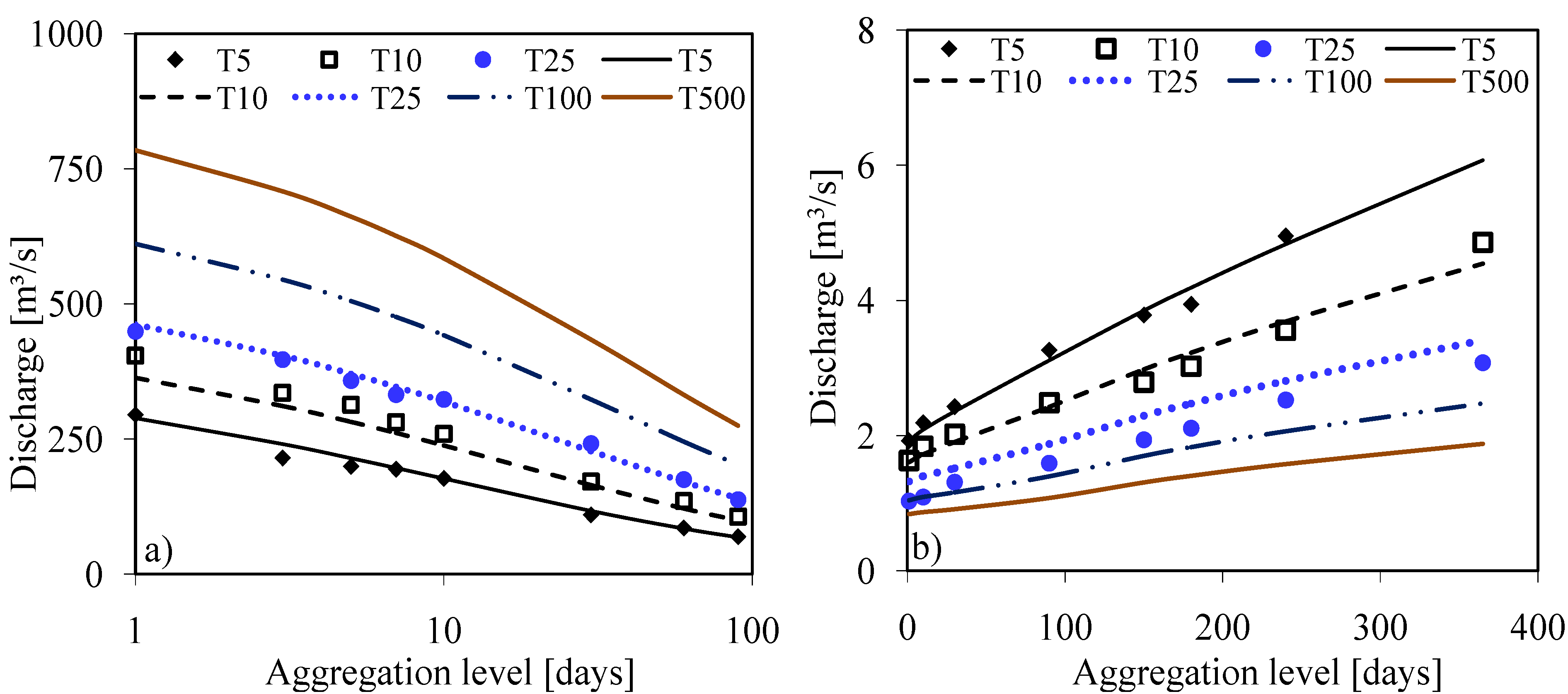
4.1. FDF Relationships
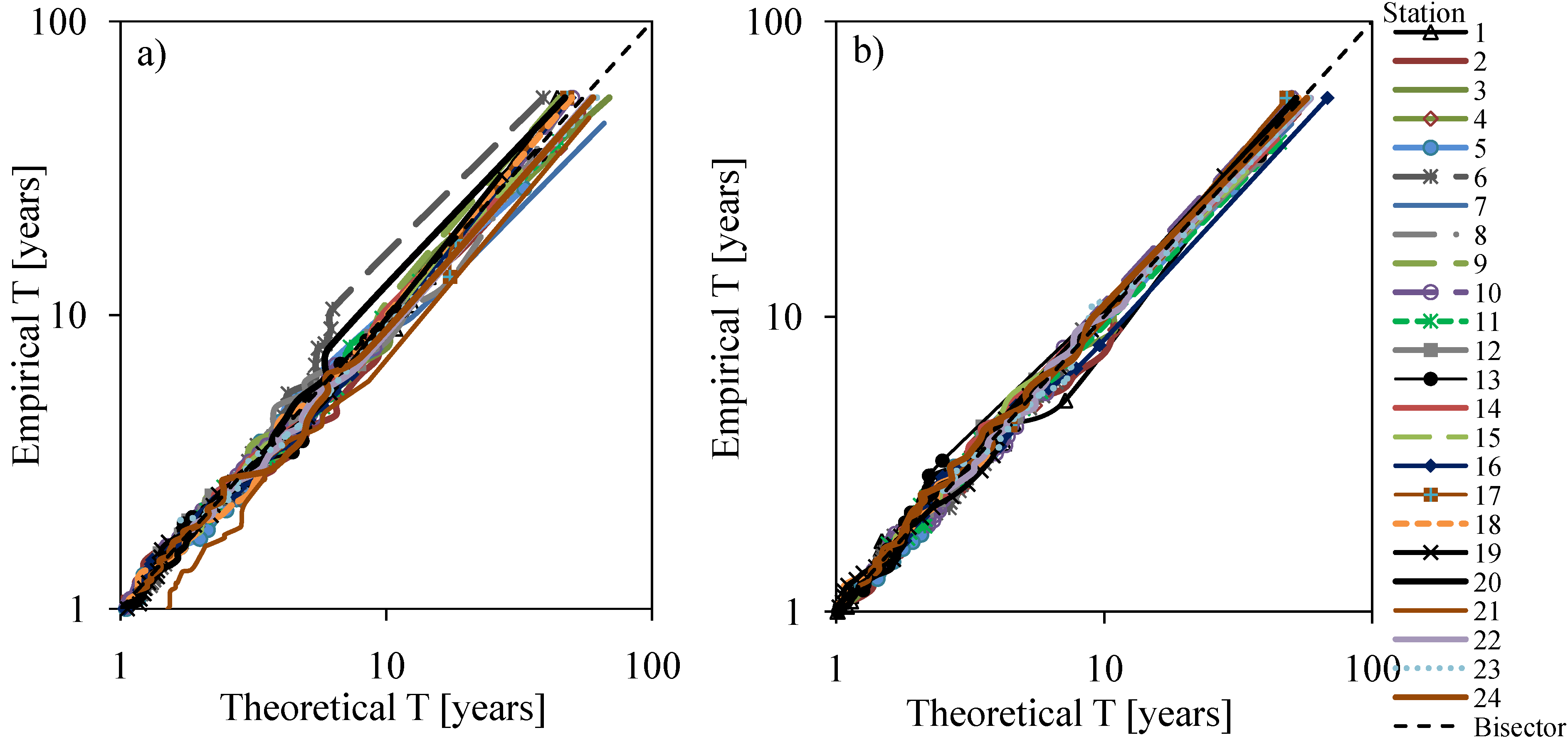
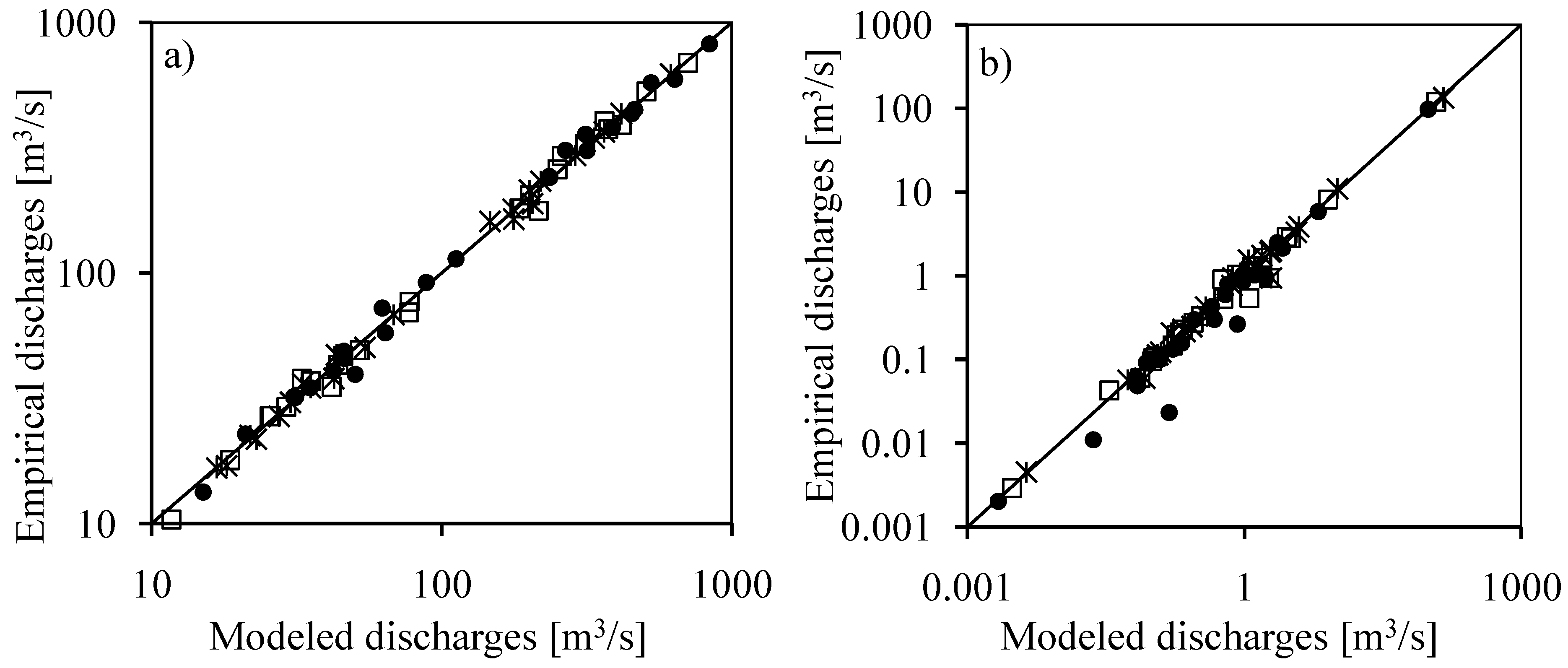
4.2. Evaluation of the FDF Relationships
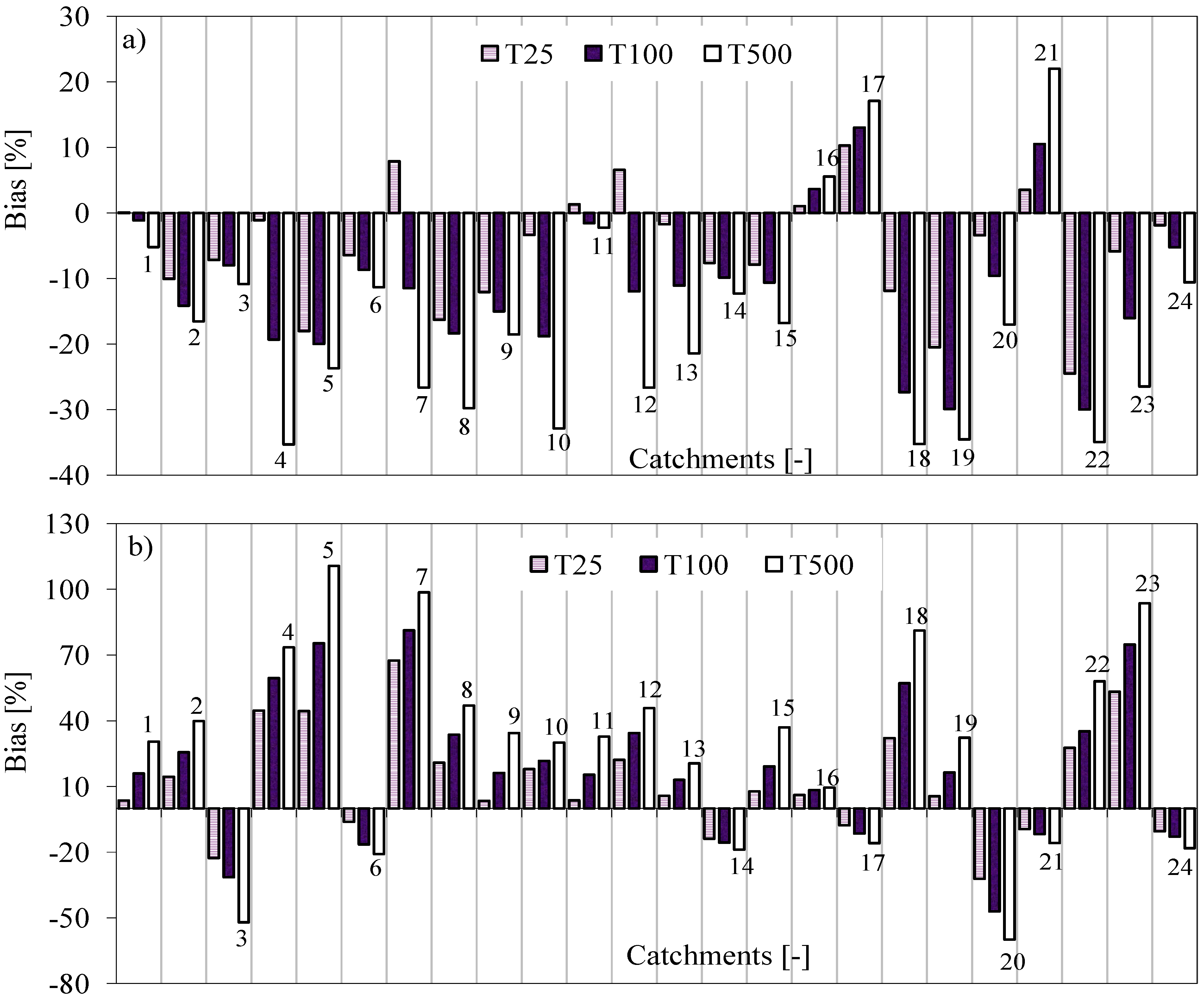
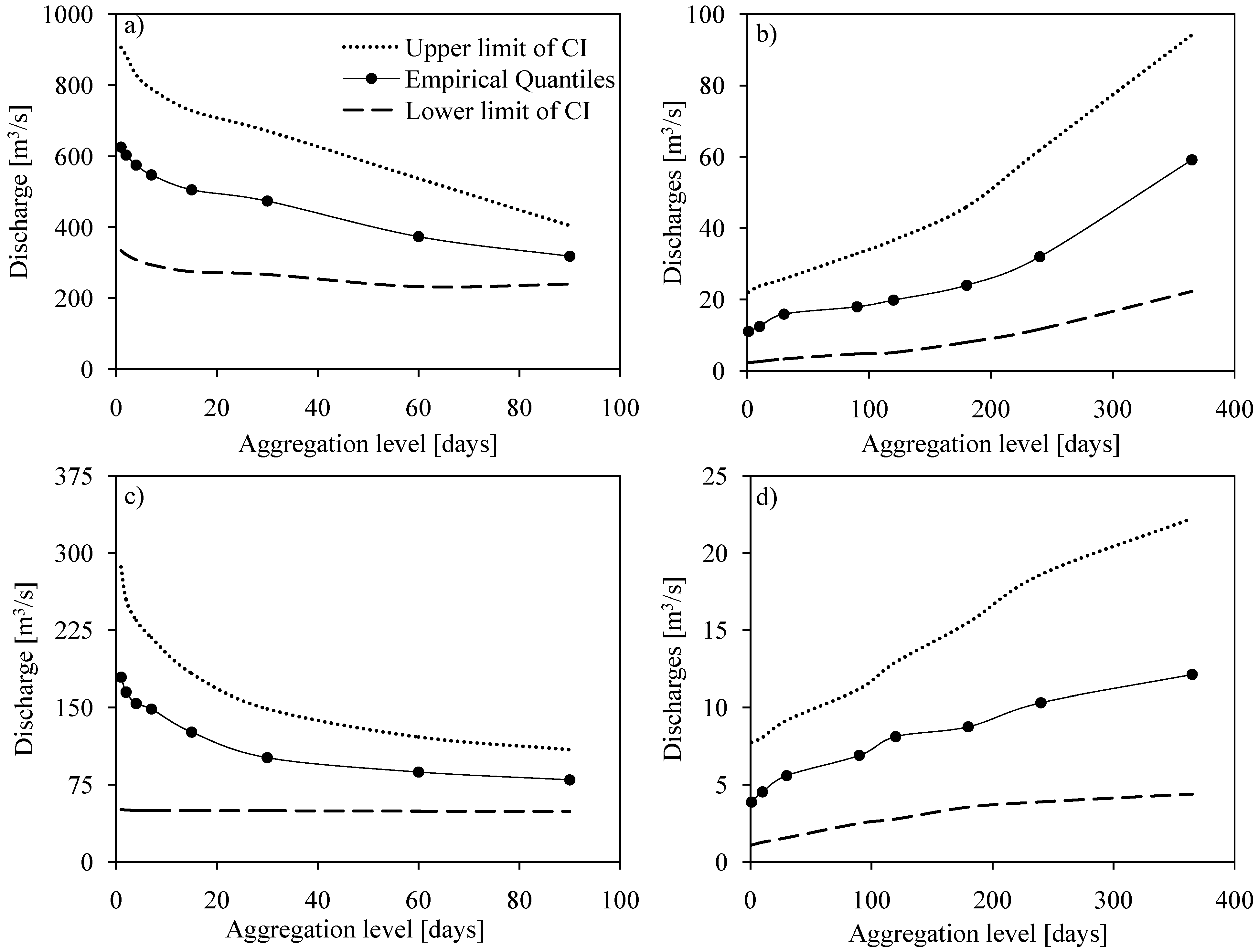
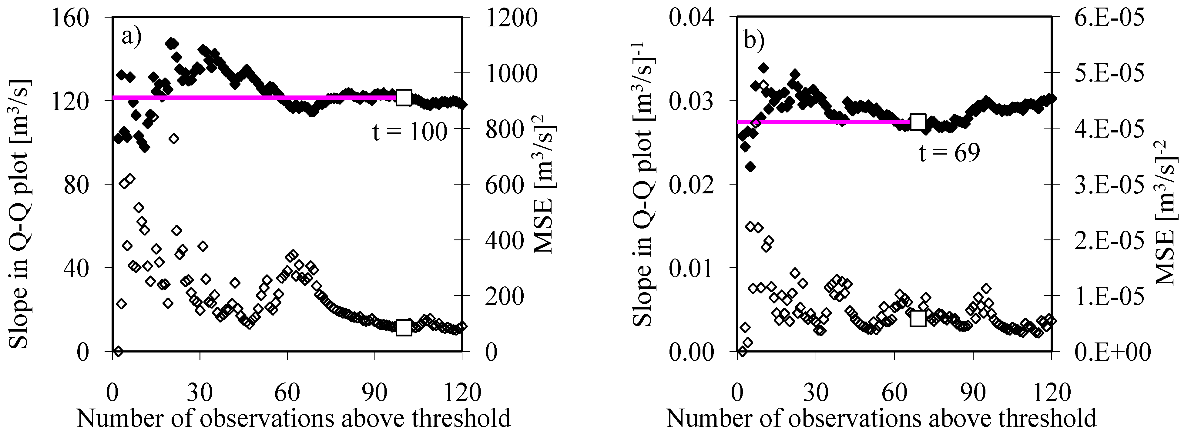
4.3. Uncertainty Analysis
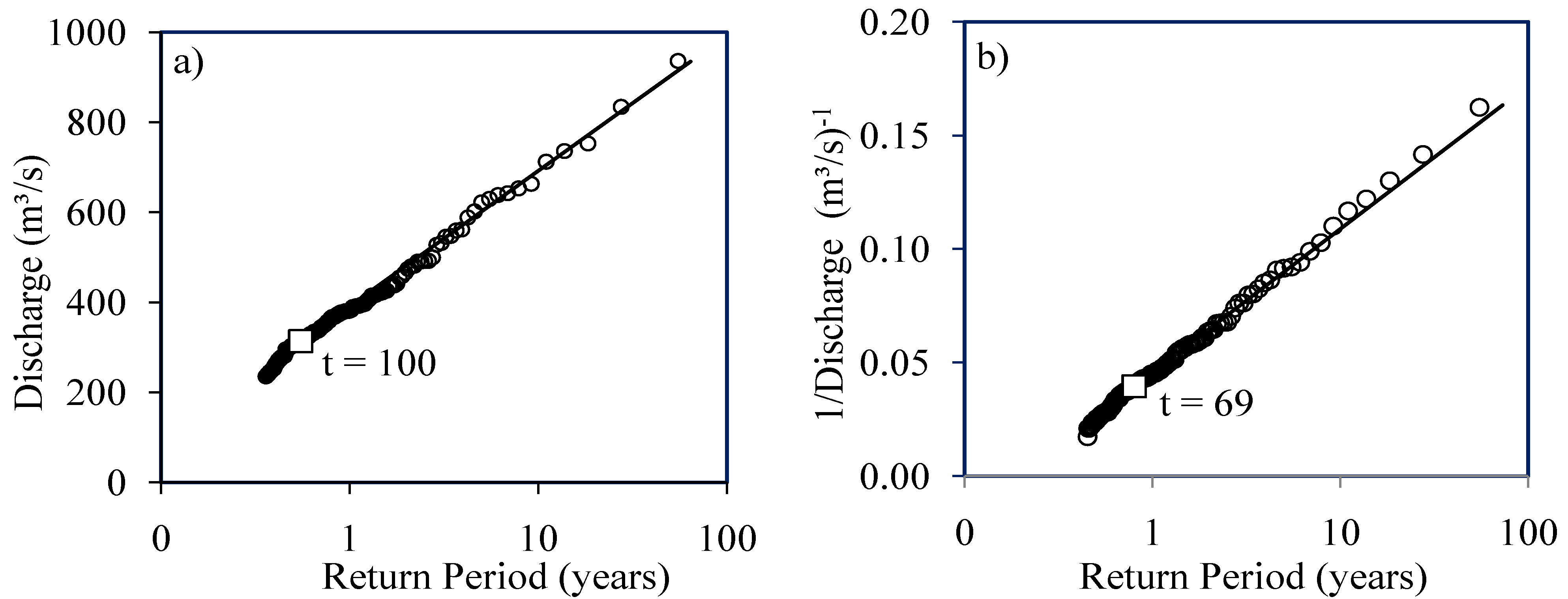
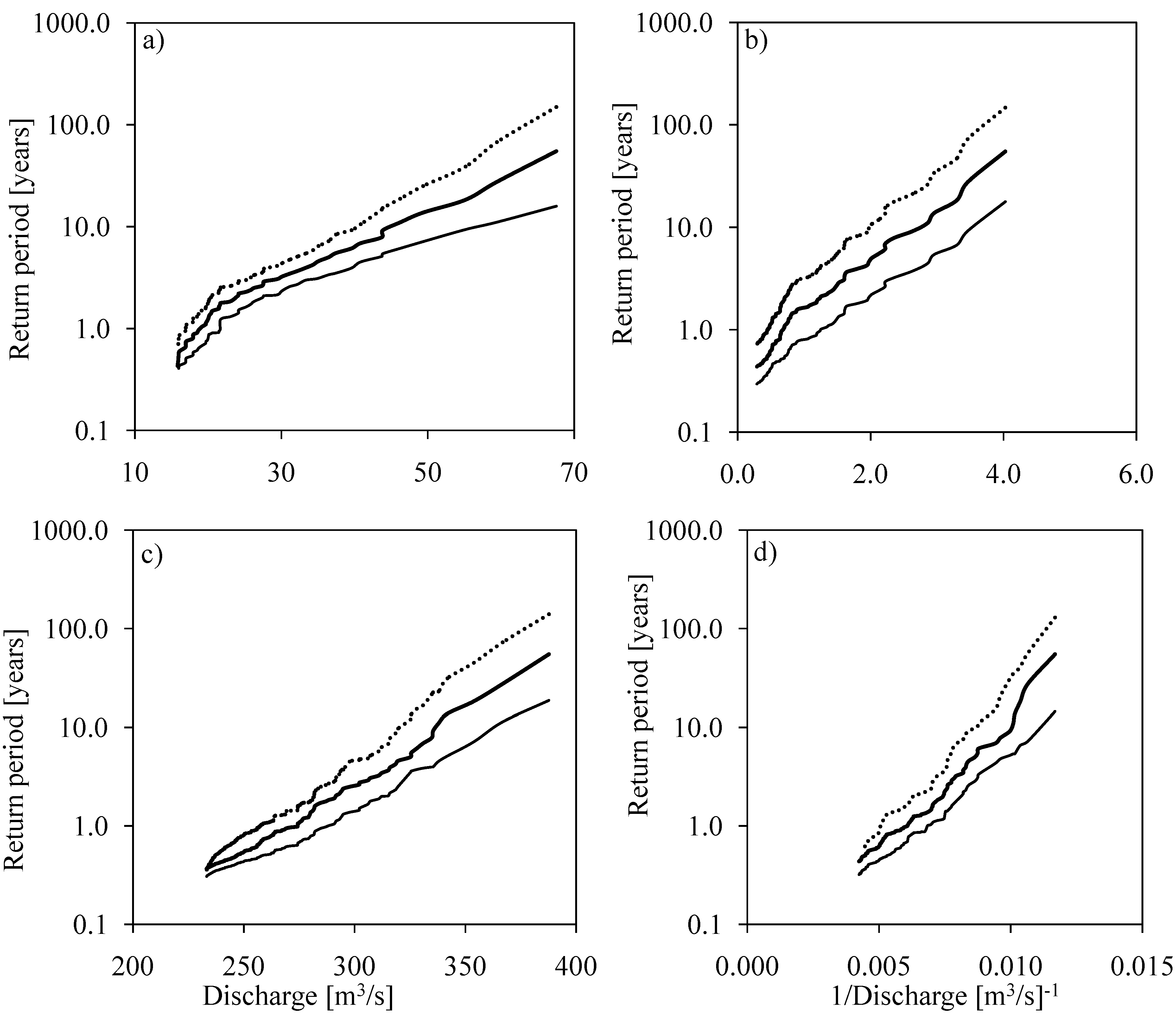
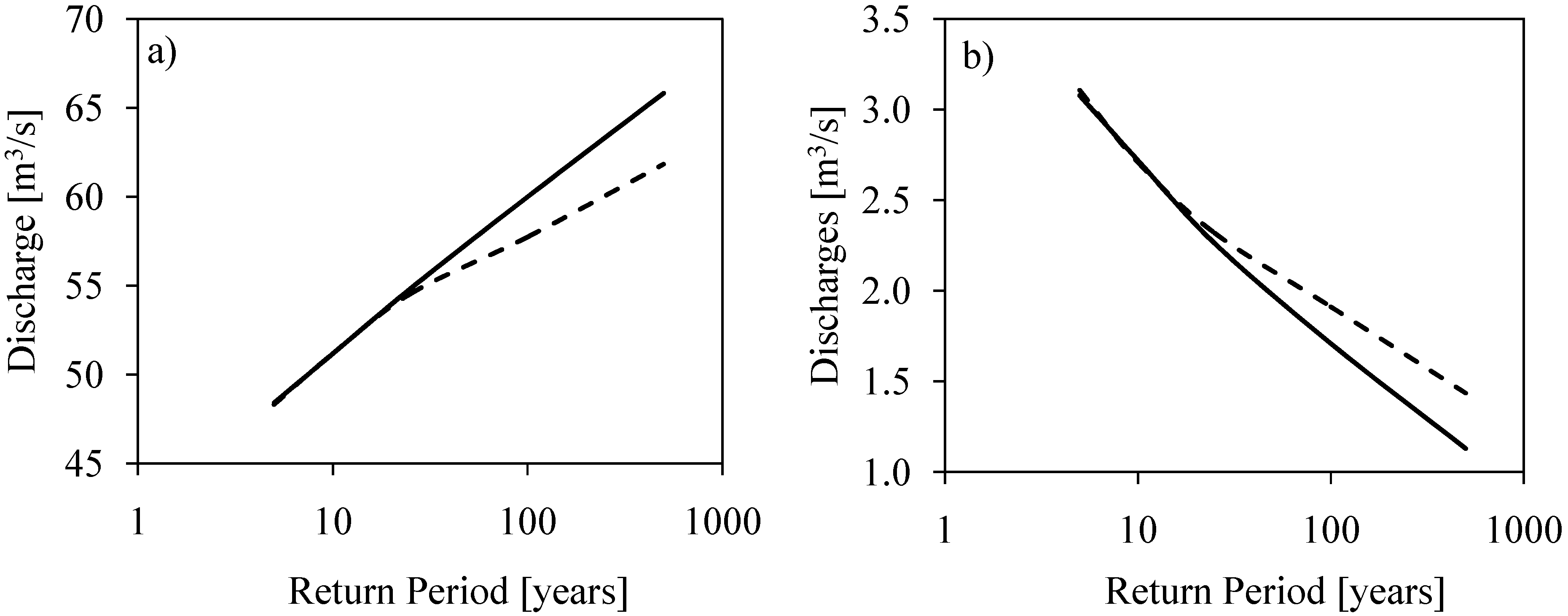
4.3.1. Uncertainty in Return Periods


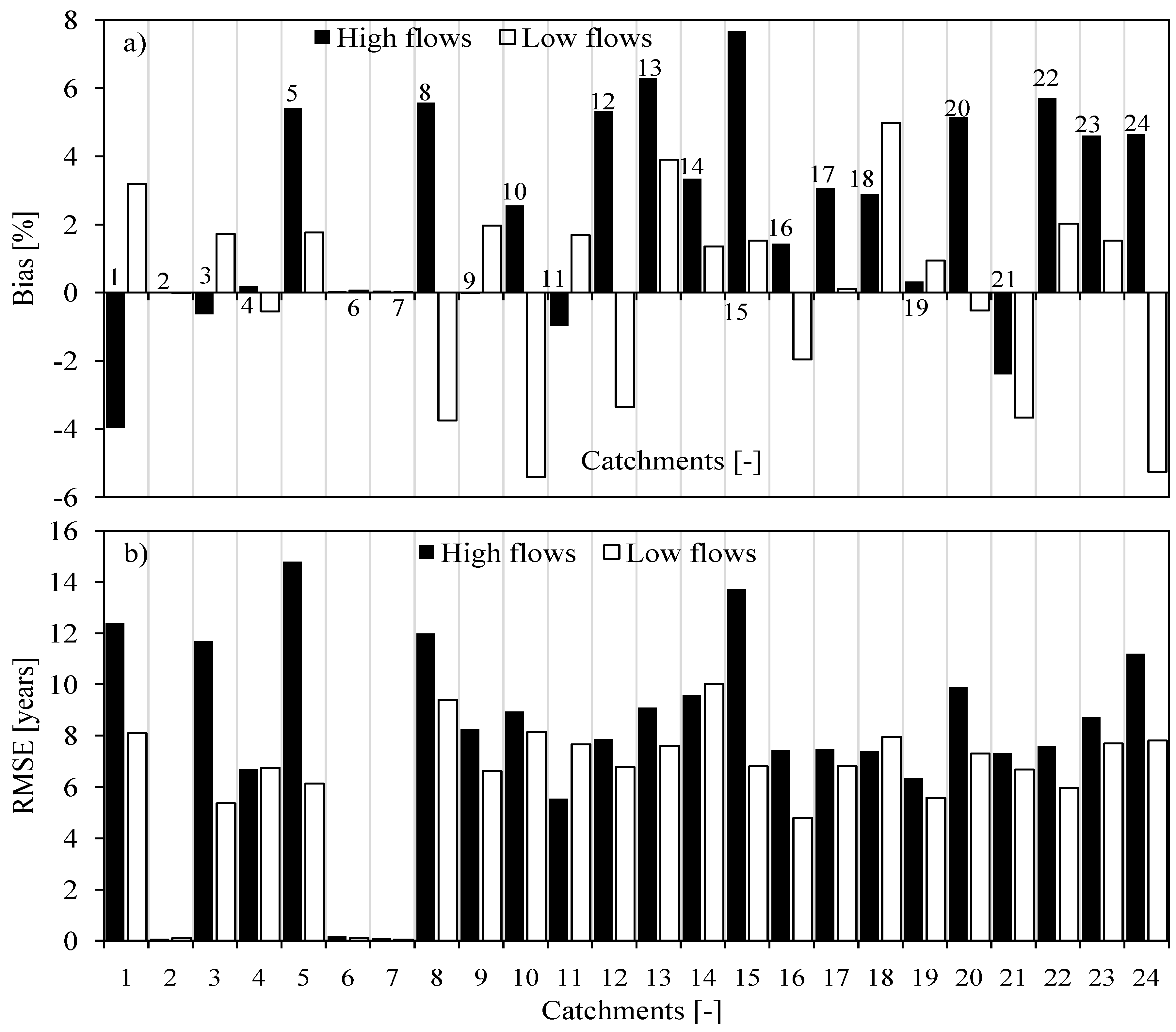

4.3.2. Uncertainty in Flow Quantiles


5. Conclusions
Acknowledgments
Conflicts of Interest
References
- Chow, V.T.; Maidment, D.R.; Mays, L.W. Applied Hydrology; McGraw-Hill: New York, NY, USA, 1988; pp. 380–410. [Google Scholar]
- Javelle, P.; Grésillon, J.M.; Galéa, G. Discharge-duration frequency curves modeling for floods and scale invariance. C.R. Acad. Sci. IIA 1999, 329, 39–44. [Google Scholar]
- Javelle, P.; Ouarda, T.B.M.J.; Lang, M.; Bobée, B.; Galéa, G.; Grésillon, J.M. Development of regional flood-duration frequency curves based on the index-flood method. J. Hydrol. 2002, 258, 249–259. [Google Scholar] [CrossRef]
- Zaidman, M.D.; Keller, V.; Young, A.R.; Cadman, D. Flow-duration-frequency behavior of British rivers based on annual minima data. J. Hydrol. 2003, 277, 195–213. [Google Scholar] [CrossRef]
- Maurino, M.F. Generalized rainfall-duration-frequency relationships: Applicability in different climatic regions of Argentina. J. Hydrol. Eng. 2004, 9, 269–274. [Google Scholar] [CrossRef]
- Borga, M.; Vezzani, C.; Fontana, G.D. Regional rainfall depth-duration-frequency equations for an Alpine region. Nat. Hazards 2005, 36, 221–235. [Google Scholar] [CrossRef]
- Juraj, M.C.; Taha, B.M.J.O. Regional flood-rainfall duration-frequency modeling at small ungaged sites. J. Hydrol. 2007, 345, 61–69. [Google Scholar] [CrossRef]
- Taye, M.T.; Willems, P. Influence of climate variability on representative QDF predictions of the upper Blue Nile Basin. J. Hydrol. 2011, 411, 355–365. [Google Scholar] [CrossRef]
- Onyutha, C. Statistical modelling of FDC and return periods to characterise QDF and design threshold of hydrological extremes. J. Urban Environ. Engng. 2012, 6, 140–156. [Google Scholar]
- Willems, P. Compound intensity/duration/frequency-relationships of extreme precipitation for two seasons and two storm types. J. Hydrol. 2000, 233, 189–205. [Google Scholar] [CrossRef]
- Nhat, L.M.; Tachikawa, Y.; Takara, K. Establishment of intensity-duration-frequency curves for precipitation in the monsoon area of Vietnam. Ann. Disas. Prev. Res. Inst. Kyoto Univ. 2006, 49, 93–103. [Google Scholar]
- World Meteorological Organization (WMO), Management of water resources and application of hydrological practices. In Guide to Hydrological Practices; WMO report No.168; WMO: Geneva, Switzerland, 2009; p. 302.
- Willems, P. A spatial rainfall generator for small spatial scales. J. Hydrol. 2001, 252, 126–144. [Google Scholar] [CrossRef]
- Peck, A.; Prodanovic, P.; Simonovic, S.P.P. Rainfall intensity duration frequency curves under climate change: City of London, Canada. Can. Water Resour. J. 2013, 37, 177–189. [Google Scholar]
- Mailhot, A.; Duchesne, S.; Caya, D.; Talbot, G. Assessment of future change in intensity-duration-frequency (IDF) curves for Southern Quebec using Canadian Regional Climate Model (CRCM). J. Hydrol. 2007, 347, 197–210. [Google Scholar] [CrossRef]
- Kuo, C.C.; Jahan, N.; Gizaw, M.S.; Gan, T.Y.; Chan, S. The Climate Change Impact on Future IDF Curves in Central Alberta. In Proceedings of Engineering Institute of Canada (EIC) Climate Change Technology Conference, Concordia University, Montreal, Canada, 27–29 May 2013.
- Nyeko-Ogiramoi, P. Climate Change Impacts on Hydrological Extremes and Water Resources in Lake Victoria Catchments, Upper Nile Basin. Ph.D. Thesis, Arenberg Doctoral School of Science, Engineering and Technology, Katholieke Universiteit Leuven, Leuven, Belgium, 2011. [Google Scholar]
- Willems, P. Revision of urban drainage design rules after assessment of climate change impacts on precipitation extremes at Uccle, Belgium. J. Hydrol. 2013, 496, 166–177. [Google Scholar] [CrossRef]
- Yu, P.S.; Yang, T.C.; Wang, Y.C. Uncertainty analysis of regional flow duration curves. J. Water Resour. Plann. Manag. 2002, 128, 424–430. [Google Scholar] [CrossRef]
- Castellarin, A.; Camorani, G.; Brath, A. Predicting annual and long term flow-duration curves in ungauged basins. Adv. Water Resour. 2007, 30, 937–953. [Google Scholar] [CrossRef]
- Ayyub, B.M. The philosophical and theoretical basis for analyzing and modeling uncertainty and ignorance. In Applied Research in Uncertainty Modeling and Analysis; Springer: New York, NY, USA, 2005; pp. 1–18. [Google Scholar]
- Davidson, A.C.; Hinkley, D.V. Bootstrap Methods and Their Application; Cambridge University Press: Cambridge, UK, 1997; p. 582. [Google Scholar]
- Mbungu, W.; Ntegeka, V.; Kahimba, F.C.; Taye, M.; Willems, P. Temporal and spatial variations in hydro-climatic extremes in the Lake Victoria basin. Phys. Chem. Earth 2012, 50–52, 24–33. [Google Scholar] [CrossRef]
- Chu, P.; Wang, J. Modeling return periods of tropical cyclone intensities in the vicinity of Hawaii. J. Appl. Meteorol. 1998, 37, 951–960. [Google Scholar] [CrossRef]
- Taye, M.T.; Willems, P. Temporal variability of hydroclimatic extremes in the Blue Nile basin. Water Resour. Res. 2012, 48, W03513. [Google Scholar]
- Nyeko-Ogiramoi, P.; Willems, P.; Gaddi-Ngirane, K. Trend and variability in observed hydrometeorological extremes in the Lake Victoria basin. J. Hydrol. 2013, 489, 56–73. [Google Scholar] [CrossRef]
- Tukey, J. Bias and confidence in not quite large samples (abstract). Ann. Math. Stat. 1958, 29, 614. [Google Scholar] [CrossRef]
- Hartigan, J. Using subsample values as typical values. J. Am. Stat. Assoc. 1969, 64, 1303–1317. [Google Scholar] [CrossRef]
- Efron, B. Bootstrap methods: Another look at jackknife. Ann. Stat. 1979, 7, 1–26. [Google Scholar] [CrossRef]
- Beven, K.J.; Binley, A.M. The future of distributed models: Model calibration and uncertainty prediction. Hydrol. Process. 1992, 6, 279–298. [Google Scholar] [CrossRef]
- Montanari, A. Uncertainty of hydrological predictions. In Treatise on Water Science; Wilderer, P., Ed.; Academic Press: Oxford, UK, 2011; pp. 459–478. [Google Scholar]
- Gichere, S.K.; Olado, G.; Anyona, D.N.; Matano, A.S.; Dida, G.O.; Abuom, P.O.; Amayi, A.J.; Ofulla, A.V.O. Effects of drought and floods on crop and animal losses and socio-economic status of households in the Lake Victoria Basin of Kenya. J. Emerg. Trends Econ. Manag. Sci. 2013, 4, 31–41. [Google Scholar]
- Kibiiy, J.; Kivuma, J.; Karogo, P.; Muturi, J.M.; Dulo, S.O.; Roushdy, M.; Kimaro, T.A.; Akiiki, J.B.M. Flood and Drought Forecasting and Early Warning; Flood Management Research Cluster, Nile Basin Capacity Building Network (NBCBN-SEC) Office: Cairo, Egypt, 2010; p. 68. [Google Scholar]
- Kenyan Ministry of Water and Irrigation (KMWI), Flood Mitigation Strategy; KMWI: Nairobi, Kenya, June 2009; p. 66.
- Awange, J.L.; Aluoch, J.; Ogallo, L.; Omulo, M.; Omondi, P. An assessment of frequency and severity of drought in the Lake Victoria region (Kenya) and its impact on food security. Clim. Res. 2007, 33, 135–142. [Google Scholar] [CrossRef]
- Otieno, H.O.; Awange, J.L. Energy Resources in East Africa; Springer-Verlag: Berlin, Germany, 2006. [Google Scholar]
- Willlems, P. A time series tool to support the multi-criteria performance evaluation of rainfall-runoff models. Environ. Model. Softw. 2009, 24, 311–321. [Google Scholar] [CrossRef]
- Csörgö, S.; Deheuvels, P.; Mason, D. Kernel estimators of the tail index of a distribution. Ann. Statist. 1985, 13, 1050–1077. [Google Scholar] [CrossRef]
- Beirlant, J.; Teugels, J.L.; Vynckier, P. Practical Analysis of Extreme Values; Leuven University Press: Leuven, Belgium, 1996. [Google Scholar]
- Willems, P.; Guillou, A.; Beirlant, J. Bias correction in hydrologic GPD based extreme value analysis by means of a slowly varying function. J. Hydrol. 2007, 338, 221–236. [Google Scholar] [CrossRef]
- Willems, P. Hydrological applications of extreme value analysis. In Hydrology in a Changing Environment; Wheater, H., Kirby, C., Eds.; John Wiley & Sons: Chichester, UK, 1998; pp. 15–25. [Google Scholar]
- Jenkinson, A.F. The frequency distribution of the annual maximum (or minimum) of meteorological elements. Q. J. Roy. Meteor. Soc. 1955, 81, 158–171. [Google Scholar] [CrossRef]
- Pickands, J. Statistical inference using extreme order statistics. Ann. Stat. 1975, 3, 119–131. [Google Scholar] [CrossRef]
- Hill, B.M. A simple and general approach to inference about the tail of a distribution. Ann. Stat. 1975, 3, 1163–1174. [Google Scholar] [CrossRef]
- Willems, P. Formula for the Calibration of QDF-Curves on the Basis of Scaling Properties and Correct Asymptotic Properties; Katholieke Universiteit Leuven: Leuven, Belgium, 2003. [Google Scholar]
- Klemeš, V. Tall tales about tails of hydrological distributions. II. J. Hydrol. Eng. 2000, 5, 232–239. [Google Scholar] [CrossRef]
- Kangieser, P.C.; Blackadar, A. Estimating the likelihood of extreme events. Weatherwise 1994, 47, 38–40. [Google Scholar]
- Nyeko-Ogiramoi, P.O.; Willems, P.; Mutua, F.; Moges, S.A. An elusive search for regional flood frequency estimates in the River Nile basin. Hydrol. Earth Syst. Sci. 2012, 16, 3149–3163. [Google Scholar] [CrossRef] [Green Version]
© 2013 by the authors; licensee MDPI, Basel, Switzerland. This article is an open access article distributed under the terms and conditions of the Creative Commons Attribution license (http://creativecommons.org/licenses/by/3.0/).
Share and Cite
Onyutha, C.; Willems, P. Uncertainties in Flow-Duration-Frequency Relationships of High and Low Flow Extremes in Lake Victoria Basin. Water 2013, 5, 1561-1579. https://doi.org/10.3390/w5041561
Onyutha C, Willems P. Uncertainties in Flow-Duration-Frequency Relationships of High and Low Flow Extremes in Lake Victoria Basin. Water. 2013; 5(4):1561-1579. https://doi.org/10.3390/w5041561
Chicago/Turabian StyleOnyutha, Charles, and Patrick Willems. 2013. "Uncertainties in Flow-Duration-Frequency Relationships of High and Low Flow Extremes in Lake Victoria Basin" Water 5, no. 4: 1561-1579. https://doi.org/10.3390/w5041561
APA StyleOnyutha, C., & Willems, P. (2013). Uncertainties in Flow-Duration-Frequency Relationships of High and Low Flow Extremes in Lake Victoria Basin. Water, 5(4), 1561-1579. https://doi.org/10.3390/w5041561